Localized and periodic exact solutions to the nonlinear Schrodinger equation with spatially modulated parameters: Linear and nonlinear lattices

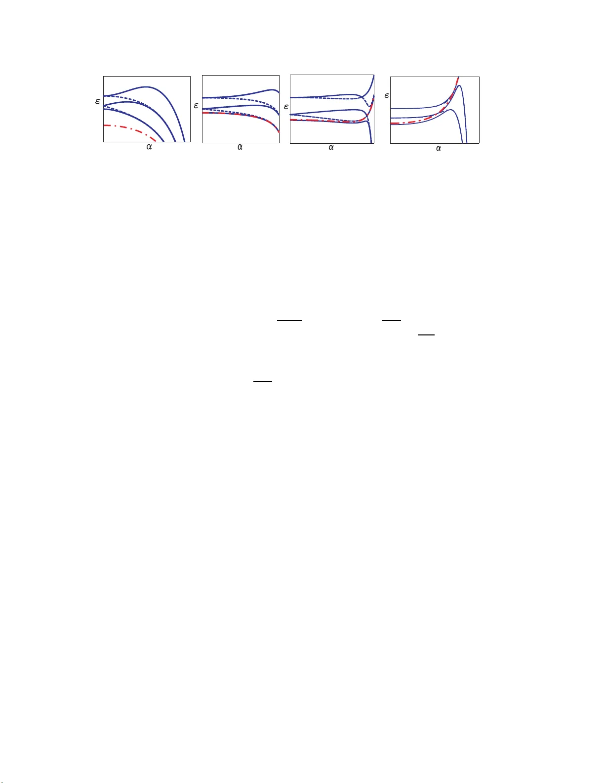
Lo calized and p erio dic exact solutions to the nonline ar Sc hr¨ odinger equatio n with spatially mo du lated p arameters: Lin ear and nonl inear lattices. Juan Belmonte-Beitia a , Vladimi r V. Konotop b , V ´ ıctor M. P ´ erez-Garc ´ ı a a V adym E. V ekslerc hi k a a Dep arta mento de Matem´ atic as, E . T. S. de Ingenier os Industriales and Instituto de Matem´ atic a A plic ada a la Ciencia y la Ingenier ´ ıa (IMACI), Universidad de Castil la-L a M ancha 13071 Ciudad R e al, Sp ain. b Dep artamento de F ´ ısic a, F aculdade de Ciˆ encias, Universidade de Lisb o a, Camp o Gr ande, Ed. C8, Piso 6, Lisb o a 1749-016, Portugal and Centr o de F ´ ısic a T e´ oric a e Computaciona l, Universidade de Lisb o a, Complexo Inter disciplinar, Avenida Pr ofessor Gama Pinto 2, Lisb o a 1649-003, Portugal. Abstract Using similarit y transf ormations we construct explicit solutions of the n on lin ear Sc hr¨ od in ger e qu ation with li n ear and nonlinear p erio dic p oten tials. W e present ex- plicit forms o f spatially lo calized and p erio dic solutions, and study their prop erties. W e pu t ou r results in the framework of the exp loited p ertur bation tec hniques and discuss their implications on the prop erties of asso ciated linear p erio dic p oten tials and on the p ossibilities of stabilizatio n of gap solitons using p olyc hromatic lattices. Key wor ds: Nonlinear lattices, nonlinear Sc hr ¨ od in ger equation, similarit y transformation, localized mo des, Bloch functions. 1 In tro duction The significan t increase of the interes ting prop erties of the solutions of the nonlinear Sc hr¨ odinger (NLS) equation with a p erio dic p oten tial during the last decade w as strongly stim ulated b y the application of that mo del in the theory o f Bose-Einstein condensates (BECs) (see e.g. [1,2]), where the mo del is kno wn also a s the Gross-Pitaevskii equation. The ma jor a dv antage of the use of o pt ical lattices, which constitute the ph ysical origin of the p erio dic Preprint submitted to Elsevier 12 Nov ember 2018 p oten tial, is the p ossibility of c hange o f their c haracteristics in space what stim ulated studies of manag ing soliton dynamics by spatially inhomogeneous lattices [3], b y lo w-dimensional lattices [4], b y lattices with defects [5,6,7], etc. Indep enden tly recen tly the re has b een in terest on t he systematic study of nonlinear lattices [8,9,10] in a more general contex t, including not only the BEC mean-field theory but also electromagnetic w av e pro pagation in la ye red Kerr media. Subseq uent studies of the in terplay b etw een linear and no nlinear lattices [11,12 ] ha ve revealed more p eculiarities o f lo calized mo des in suc h structures and un usual stabilit y prop erties of plane w av e solutions. Searc h of the lo calized mo des in a ll the studies men tio ned ab ov e w as carried out within the framew ork of approximate and n umerical metho ds, as the mo d- els, in general case, do no w allo w for exact solutions. Ho we ve r, r ecen tly it w as realized that for a n um b er of NLS mo dels including sp ecific ty p e of p erio dic p oten tials, exact p erio dic solutions can b e constructed [1 3 ,14], what can b e done in a systematic manner, using a kind of inv erse engineering a nd start- ing with a give n p erio dic field distribution [1]. W e wan t also to men tion the Refs. [15,16,17,18], where differen t metho ds to find exact solutions to nonlinear Sc hr¨ odinger equations were studied. Ev en greater prog ress w as ac hiev ed in constructing exact solutio ns, and in particular of in tegrable mo dels, of the NLS equation with time dep enden t co efficien ts (see e.g. [19,20,21,22,23,24,25] for the work dev oted to equations of the NLS-type), and f o r the stationary GP equation with a p oten tial and v arying nonlinearit y [26,27]. How ev er, a ll men tioned mo dels allo wing f o r ex- act solutions lo ok sometimes rather artificial, for example mo dels with exact p erio dic solutions mu st b e infinite or sub ject to cyclic b oundary conditions and mo dels with trap p otentials require sp ecific la ws of time v aria tions of the co efficien ts. D espite those difficulties, they hav e tw o imp orta nt adv an tages the first b eing that they are still exp erimen tally feasible, and the second b eing that they allow for exact solutions, thus ruling out an y am biguit y in in terpretation of the phys ical phenomena. Returning to the NLS mo dels with spatially p erio dic co efficien ts, we observ e that no exact lo c a lize d solutions hav e b een rep orted, so f a r (the only w ork to our kno wledge is the a na lytical approac h for constructing sufficien tly narrow pulses, recen tly elab or ated in [28 ]) . This is the main goal of t his presen t pap er to presen t for the first t ime suc h solutions, whic h can b e obtained for sp ecific t yp es of linear and no nlinear lattices. Moreo v er, simple analysis of the pre- sen ted mo dels and their solutions will allo w us to mak e sev eral conclusions ab out prop erties of the underlying linear la t t ices and ab out stabilization of lo calized mo des b y p olyc hromatic lattices. The results presen ted in this work, represen t the extension of t he ideas elab ora ted in earlier publications [26,27] to the case of p erio dic nonlinearities. 2 The pap er is orga nized as follows . In Section 2, we dev elop the theory of similarit y tra nsformations for our mo del problem: the nonlinear Schr¨ odinger equation with a spatially inhomogeneous nonlinearit y . In Section 3, we study the stationary lo calized mo des of the inhomogeneous nonlinear Sc hr¨ odinger equation (INLSE). In Section 4, w e presen t a study o f the stability of suc h solutions. Finally , in Section 5, w e construct explicit p erio dic solutions of the INLSE and study their stabilit y . 2 Similarit y transformations W e consider the one-dimensional spatially inhomogeneous NLS equation iψ t = − ψ xx + v ( x ) ψ + g ( x ) | ψ | 2 ψ , (1) with x ∈ R , v ( x ) and g ( x ) b eing resp ectiv ely linear and nonlinear p erio dic p oten tials, whose p erio ds will b e required to b e equal. More sp ecifically , with- out loss of generality w e imp ose the p erio d to b e π : i.e. v ( x + π ) = v ( x ) and g ( x + π ) = g ( x ), what can b e alw ays achie ve d b y prop er rescaling of v a riables. (It is worth to men tion here that in the BEC theory t he choice of the p erio d π corresp o nds to the scaling where the energy is measured in the units of the recoil energy). In order to eliminate p ossible unessen t ia l constan t energy shifts and bring the stat ement of the problem closer to the standar d one w e imp o se the requiremen t for the p erio dic p ot ential to hav e a zero mean v alue, i.e. h v ( x ) i ≡ 1 π Z π 0 v ( x ) dx = 0 . (2) The complex field ψ ( t, x ) will b e referred to as a (macroscopic) w av e function, where again w e b ear in mind BEC applications. In this paper, w e fo cus on stationary solutions of Eq. (1), which are o f the form ψ ( t, x ) = φ ( x ) e − iµt , (3) where φ ( x ) is a function of x only and µ is a constant b elo w referred to as a c hemical p oten tial. As it is clear − φ xx + ( v ( x ) − µ ) φ + g ( x ) φ 3 = 0 . (4) No w, follo wing the ideas of [26,27], w e lo o k for a tra nsfor mat ion reducing Eq. (4) to the solv able stationary NLS equation E Φ = − Φ ′′ + G | Φ | 2 Φ , (5) 3 where Φ ≡ Φ( X ), a prime stands for the deriv ativ e with resp ect to X , E and G are constants, and X ≡ X ( x ) is a new spatial v ariable. T o this end, w e use the ansatz φ ( x ) = ρ ( x )Φ( X ) , (6) where Φ( X ) is a solution of the statio na ry equation (5) and b oth ρ ( x ) and X ( x ) are functions whic h must b e found from the condition that ψ ( x ) solv es Eq. (4). Substituting ( 6) in to (4) we obtain the link:  ρ 2 X x  x = 0 , (7) as w ell as expressions for g ( x ) a nd v ( x ) through ρ ( x ) and X ( x ): g ( x ) = G X 2 x ρ 2 , a nd v ( x ) = ρ xx ρ + µ − E X 2 x . (8) F rom the expres sion for g ( x ) w e find the first constrain t of the theory: the metho d is applicable to mo dels with sign definite nonlinearities, and one mus t c ho ose G =sign ( g ( x )). Next, b eing in terested in s olutio ns existing on the whole real axis and excluding singular p ot entials w e ha ve to restrict the anal- ysis to functions ρ ( x ) in C 2 ( R ) whic h do not acquire zero v alues a nd th us are sign definite. Moreo v er since neither (8 ) nor (7) c hange as ρ ( x ) c hanges the sign (what simply reflects the phase inv ariance of the mo del (4)), in what follo ws we restrict the consideration to the case ρ ( x ) > 0 . The solution of (7) is immediate: X ( x ) = Z x 0 ds ρ 2 ( s ) . (9) Here w e ha ve take n in to accoun t that the constan t of the first inte gra tion with resp ect to x can b e c hosen 1 , as fa r as ρ ( x ) is still left undefined, and the second integration constan t con v enien tly fixes the origin. Thus w e hav e X (0) = 0 , and lim x →±∞ X ( x ) = ±∞ . (10) No w the co efficien ts in Eq. (4) can b e rewritten in the for m v ( x ) = ρ xx ρ − E ρ 4 + µ, g ( x ) = G ρ 6 . (11) 4 Th us, (6 ) with (9) giv es a solution of Eq. (4), whic h dep ends on the the p ositiv e definite function ρ ( x ), which m ust b e c hosen π -p erio dic. This choice is naturally v ery rich. T o b e sp ecific w e in v estigate in detail the simplest case where ρ ( t, x ) = 1 + α cos(2 x ) , (12) with α b eing a real constant, suc h that | α | < 1, and resp ectiv ely v ( x ) = − 4 α cos(2 x ) 1 + α cos(2 x ) − E (1 + α cos(2 x )) 4 + µ, (13) g ( x ) = G (1 + α cos(2 x )) 6 , (14) where µ is c hosen to ensure (2) and reads µ = 4 − 4 √ 1 − α 2 + E 2 + 3 α 2 2(1 − α 2 ) 7 / 2 . (15) Some direct generalizations of this mo del are presen ted in the App endix. The introduced linear p erio dic p oten tial v ( x ) has a num b er of p eculiar prop- erties, some o f whic h are: (i) It allows for some par t icular explicit forms of the Blo c h function (see e.g. expressions ( 1 8) and (2 7), b elo w), what is a ra t her p eculiar situation since in a general situation explicit for ms of solutions of a Hill equation in terms of the elemen tary fucntions are not a v ailable. (ii) α app ears to b e the para meter allowing one to con trol the band sp ectrum (as this is illustrated in each of the panels in Fig. 1 b elo w) and, in particular, allo wing for smo oth tra nsition b etw een con tinuum sp ectrum (at α = 0 where the p erio dic p otential do es not exist and the discrete sp ectrum (at | α | = 1 where the p erio dic p o ten tial is represen ted b y a sequence of p oten tial wells of infinite depths). In Fig . 1 these tw o situations are express ed by the f a ct that all gaps are collapsed at α = 0, one the one hand, and one of the bands acquire an infinite width at α = 1, on t he other hand. (iii) By v arying the par ameter E one can transform the p otential from a general for m with no in terv als of c o existenc e ( E < 0) to a form with c o ex is- tenc e ( E > 0) . Hereafter, follow ing [31] under the co existence phenomenon w e understand the o ccurrence when an inte rv al of instability (i.e. a gap) dis- app ears due t o collapsing of tw o gap edges. This prop ert y is also illustrated in Fig. 1, where panels (a) and (b) corresp ond to the general situation while in the pa nes (c) and ( d) one o bserv es in tersection of a dashed-doted (red) line with the gap edges precisely in the co-existence p oin ts. It is remark a ble that these prop erties b ecome more clear departing from the 5 solution of the resp ectiv e nonlinear problem. W e consider them in the next sections. 3 Stationary lo calized mo des W e start with the analysis o f the lo calized mo des. T o this end w e imp o se the b oundar y conditions lim x →±∞ φ ( x ) = 0 and taking in to accoun t (6) and (10) w e conclude that Φ( X ) m ust satisfy the zero b o undary conditions, as w ell: lim X →±∞ Φ( X ) = 0. This is the case where G = − 1 and Φ( X ) = √ − 2 E / cosh( √ − E X ) i.e. Φ( X ) is the standar d stationary NLS soliton. The resp ectiv e solution o f Eq. (4) reads φ s ( x ) = √ − 2 E 1 + α cos(2 x ) cosh( √ − E X ( x )) , X ( x ) = Z x 0 ds (1 + α cos(2 s )) 2 . (16) Let us no w consider in more detail t he obtained solution. First of all w e recall that the che mical p oten tial of a n y stationary solution of the NLS equation with a p erio dic p oten tial, whic h tends to zero or acquires a zero v alue m ust b elong to a forbidden g a p of the resp ectiv e p o ten tial and suc h solutions ha ve a space- indep enden t phase, a nd th us can b e c hosen real ( see e.g. [1,29]). The o btained solution (16) has che mical p oten tial µ , giv en by Eq. (15), and hence it m ust b elong to a ga p of the sp ectrum of the p oten tia l v ( x ), which is determined by the Hill eigen v alue problem: − ϕ xx + v ( x ) ϕ = E ϕ . (17) Moreo v er, since the obtained solution (16) exists for arbitrar y negative E , including the limit where E → −∞ and conseq uently µ < v ( x ) one concludes that E = µ b elongs to the semi-infinite gap ( −∞ , E ( − ) 1 ) of the band sp ectrum of v ( x ), i.e. E ( − ) 1 > µ , where w e use the notations E ( − ) n and E (+) n for the lo we r and upp er edges of the n -t h band, i.e. stabilit y region, pro vided that α = 1 designates the low est band. Indeed, a ssuming the opp osite, i.e. assuming that at some negativ e energy the solution b elongs to one of the finite gap and taking into accoun t the con tinuous dep endence o n E o ne concludes tha t at some negative E , the c hemical p oten tia l (15) crosses the stability region, what con tradicts to the existence of t he solution with zero b oundary conditions. Alternativ ely , t he ab ov e conclusion follows f o rm the facts that at α = 0 the solution (16) is in the semi-infinite ga p and that the dep endence of µ and v ( x ) on the parameter α ∈ ( − 1 , 1) is contin uous. The describ ed phenomenon is illustrated in Fig . 1 (sp ecifically in the panel (a)) where w e sho w the edges of the lo w est bands vs the para meter α for four t ypical situations E < 0 (panel (a)); E = 0 (panel (b)); E ∈ (0 , E 0 ) with 6 0 0.6 -8 0 4 8 (a) -8 8 0 0 4 0.9 (b) -4 0 4 8 (c) 0 0.8 -8 4 32 16 (d) 0 0.8 Fig. 1. Boundaries of the lo w est band edges (5 firs t b and edges) of the sp ectrum of Eq. (17) as fun ctions of α f or (a) E = − 5 (b) E = 0, (c) E = 0 . 1, and (d) E = 1. Solid and dash ed lines corresp ond to E ( − ) n and to E (+) n . The (red ) dashed-dot lines represent th e c h emical p oten tial µ . E 0 = max α { E m ( α ) } = 2 / 5 and E m ( α ) = 8(1 − α 2 ) 3 / (20 + 15 α 2 ) b eing the p oin t of the lo cal minim um of the c hemical p oten tial ∂ µ/∂ E | E = E 0 = 0 for a giv en α , (panel (c)), a nd E > E 0 (panel (d)). Lea ving the discussion of the situations depicted in Fig. 1 (c), (d) for Sec. 5, no w we turn to the limiting cases of the solution ( 16). At E → −∞ it ap- proac hes the NLS soliton: φ s ( x ) ∼ √ − 2 E (1 + α ) / cosh( √ − E (1 + α ) x ), what reflects the f a ct that the lo calization region, determined by 1 / q | E | , is m uc h smaller than the p erio d of the p oten tial. Th us ( 1 6) is an example of an exact solution, whose approximate form can b e obta ined as suggested in [28] (after the scaling o ut the amplitude √ − E ). An ev en more in teresting situation corresp onds to small | E | . When | E | → 0 the c hemical p oten tial approach es the band edge, what is illustrated in F ig . 1 (b), where E = µ coincides with the edge o f the semi-infinite band (in other w ords, here we are dealing with a situation where a for m ula for dep endence of the low est band edge on the parameters of the problem is giv en explicitly b y (15)). As it is w ell kno wn (see e.g. [1,29] and references therein) in this case the solution is accurately describ ed b y the m ultiple-scale approxim at io n and represen t s an en v elop e of the Blo ch state corr esp o nding to the gap edge. The structure of (16) implies that Φ( X ) is the en v elop e while ϕ ( x ) = 1 + α cos(2 x ) , (18) is the exact Blo c h function of the p oten tial v ( x, 0), give n b y (13), whic h cor- resp onds to the lo w est edge of the first band. In other w ords, in the limit | E | → 0 , (16) is an ex act envelop e soliton s olution bifurcating from the edge of the linear sp ectrum (to the b est of authors kno wledge (16) is the first kno wn solution of suc h a t yp e). In Fig. 2 w e illustrate the t wo opp osite limits of (16 ) corresp onding to an en v elop e (panel a) and to a narro w (panel b) NLS-type soliton. Finally w e observ e that b y changing the parameter α , one can scan the semi- 7 -80 80 0 -40 40 0 0.1 0.2 x (a) -10 10 0 0 3.5 x (b) Fig. 2. Solutions of Eq. (4), which are giv en b y (16), for (a) E = − 0 . 01 , α = 0 . 3 and (b) E = − 5, α = 0 . 1. infinite gap, obta ining the lo calized mo de with a priori giv en detuning t ow ards the gap. 4 Stabilit y of the solutions T o c hec k the linear stabilit y of the solution (16) w e study the ev olution of small p erturbations of the form ψ ( x, t ) = ( φ ( x ) + f ( x, t ) + ih ( x, t )), where f and h a r e real functions, whic h leads to the standard linearized Schr¨ odinger equation ∂ t    f h    = N    f h    , (19) with N =    0 L − − L + 0    , (20) and L − = − ∂ xx + v ( x ) + g ( x ) φ 2 ( x ) , (21) L + = − ∂ xx + v ( x ) + 3 g ( x ) φ 2 ( x ) , (22) F or p erturbations f , h ∝ e i Ω t , w e ha ve Ω 2 f = L − L + f . (23) The op erators L − and L + are self-adjoint. In the following, we will study some prop erties of t hese op erato rs. Using the fact that φ satisfies the Eq. (4 ), one 8 -0.1 -0.5 (a) Stable zone 0.4 -0.15 E -0.4 -0.3 -0.2 -0.2 -0.3 0.1 0 0.01 -0.4 -0.4 -2 -3 -4 -5 E Stable zone (b) -1 -0.1 -0.3 -0.2 0 Fig. 3. [Color onlin e] Stable zones of the solutions (16), for different v alues of the parameters α and E (a) − 0 . 5 ≤ E ≤ − 0 . 1 (b) − 5 ≤ E ≤ − 1. easily ch eck s t hat the op erator L − can b e rewritten a s L − = − 1 φ ∂ x φ 2 ∂ x 1 φ · !! . (24) As a conseque nce, R f L − f dx = R | ∂ x  f φ  | 2 φ 2 dx ≥ 0, and the op erat o r L − is nonnegativ e. Th us, the sp ectrum of the op erator L − is comp osed of: (i) A simple eigen v alue λ − = 0, with the corresp onding ev en eigenfunction, whic h is solution o f Eq. (4). (ii) A strictly p ositive con tin uous sp ectrum [ β , ∞ ). With regard to L + op erator, it satisfies the following relation L + = L − + 2 g ( x ) φ 2 ( x ). As g ( x ) is a negativ e function, the first eigenv alue of L + , λ + , satisfies λ + < 0. So, at least, an eigenv alue of L + is negativ e. Th us, as the L − op erator is nonnegativ e but the L + op erator is nonp ositiv e, the comp osition L − L + is indefinite. Th us, w e can no t say an ything analyt- ically of the sign of Ω 2 . Moreo v er, the fact that the p otential ( 1 3) can tak e b oth p ositiv e and negativ e v a lues complicates further the a na lytical study . Therefore, we ha v e to resort to nume rical metho ds to solv e Eq. (23). If some eigen v alue Ω 2 is negativ e, the asso ciat ed solution is unstable. Other- wise, the solutio n is stable. W e can calculate the eigenv alues of the op erat o r L − L + n umerically through a direct discretization of the L − L + op erator. In Figs. 3 (a ) and (b), we sho w the stable zones of the solutions (16), for differ- en t v alues of the parameters α and E . In Fig. 3 (a), we hav e studied the case − 0 . 5 ≤ E ≤ − 0 . 1. The zones of stabilit y for the case − 5 ≤ E ≤ − 1 are show n in Fig. 3(b). T o confirm this result, w e hav e studied n umerically the ev olution of the solutions (16) under finite amplitude p erturbations. W e ha ve confirmed that these obtained solutio ns are stable in the range giv en b y Figs. 3 (a) a nd (b). 9 5 Exact quasi-p erio dic solutions Let us no w turn to (quasi-) p erio dic solutions of Eq. (4). T o this end, first, w e hav e to recall the solutions o f the NLS equation (5) whic h are expressed in terms of the Jacobian elliptic functions, for whic h w e use the standard notations [30]. While doing this w e b ear in mind that differen t functions Φ( X ) whic h are obtained b y the shift of the arg umen t (lik e, for example, in (25a) and (25 d) b elow), and th us represen ting the same solutio n of the homogeneous NLS equation, now will give or igin to essen tially differen t solutions of Eq. (4) , b ecause the latter are comp osed of the t w o p erio dic p erio dic factors steaming from the structure of t he p erio dic p oten tial (they ar e describ ed b y the function ρ ( x )) and from the NLS solutions mentioned ab ov e, (see Eq. (6)). W e start with the simplest solutions of Eq. (4) for g ( x ) < 0 (i.e. G = − 1). They are φ (1) ( x ) = √ 2 k ν (1 + α cos(2 x )) cn( ν X , k ) , ν 2 = E 1 − 2 k 2 , (25a) φ (2) ( x ) = √ 2 ν (1 + α cos(2 x )) dn( ν X , k ) , ν 2 = E k 2 − 2 , (25b) φ (3) ( x ) = q 2(1 − k 2 ) ν (1 + α cos(2 x )) 1 dn( ν X , k ) , ν 2 = E k 2 − 2 , (25c) φ (4) ( x ) = q 2(1 − k 2 ) k ν (1 + α cos(2 x )) sn( ν X , k ) dn( ν X , k ) , ν 2 = E 1 − 2 k 2 , (25d) These are real functions, what determines the regions of the parameters where they are v alid. In particular, taking in to a ccoun t that the elliptic mo dulus k ∈ [0 , 1] w e ha ve that φ (2) ( x ) a nd φ (3) ( x ) a r e v alid only fo r E < 0, i.e. these are solutions b elonging to the semi-infinite gap, while φ (1) ( x ) a nd φ (4) ( x ) b elong to the g ap E < 0 and k > 1 / √ 2 (see Fig. 1(a)) or to the band E > 0 and k < 1 / √ 2 (see Figs. 1 (c) and (d)). All the solutions bifurcate from the linear Blo c h state (18 ) reco v ered at E = 0. The simplest solutions f o r g ( x ) > 0 ( G = 1) read φ (5) ( x ) = √ 2 k ν (1 + α cos(2 x )) sn( ν X , k ) , ν 2 = E 1 + k 2 , (26a) φ (6) ( x ) = √ 2 k ν (1 + α cos(2 x )) cn( ν X , k ) dn( ν X , k ) , ν 2 = E 1 + k 2 . (26b) As it is clear these solutions are v alid for E > 0. In the ab o v e fo rm ulas (25a) – ( 2 6b), X ( x ) is defined in (16 ), and ρ ( x ) is giv en b y (12). 10 Let us no w consider the pair of solitons (26a), (26b) (or alternative ly , the pair (25a), (25d)) in the ”linear” limit k → 0. They readily giv e t w o eigenstates of the p otential v ( x ) ϕ 1 = (1 + α cos(2 x )) s in  √ E X  , (27a) ϕ 2 = (1 + α cos(2 x )) c os  √ E X  . (27b) These are linearly indep enden t solutio ns. As it is kno wn (see [31] for the details) the co existence of suc h solutions o ccurs only if one of the gaps is closed. Th us, in α -dep endence of the sp ectrum of the p oten tial v ( x ) giv en b y (13), (15) at E > 0 there m ust exits p oin ts at whic h the first low est ga p is closes and through which the c hemical p otential µ g iven b y (15) passes. This is exactly what w e observ ed in panels (c) and (d) of Fig. 1. The existence of suc h po ints at sufficien tly la rge α steams from the fact that for E > 0 the c hemical po t ential infinitely grows with α while the minima of the p erio dic p oten tial tend to −∞ . Other exact eigenstates of the p oten tial v ( x ) giv en b y (13) can b e obtained b y considering the linear limit of the solutions solutions (25c) and (25d) whic h corresp onds to k → 1. In this w a y w e o bt a in a pair of t w o ”unstable” solutions ϕ 3 = (1 + α cos(2 x )) c osh  √ − E X  , (28a) ϕ 4 = (1 + α cos(2 x )) s inh  √ − E X  . (28b) As it is clear the com binations ϕ 3 ± ϕ 4 supplied b y the prop er constan t factor pro vide the asymptotics o f the solitary w av e φ s ( x ) giv en by ( 1 6) a t x → ∓∞ . T aking into accoun t that g ( x ) is sign definite, simple stability a na lysis of the presen ted solutions can b e p erformed following [14]: since φ (2) ( x ) > 0 and φ (3) ( x ) > 0 one verifies that they are linearly unstable, while the stabilit y of the solutions φ (1) ( x ), φ (4) ( x ), φ (5) ( x ) and φ (6) ( x ) is left undetermined. Finally , w e consider the limit k → 1 / √ 2 of the solutions (25a) and (25 d), whic h corresp onds to the limit o f large nonlinearity . F or this case, the p ot ential v ( x ) can b e view ed as a small and smo oth p erturbation o f the NLS equation, whose nonlinearit y is also a slo w function of the spatial v ariable. Th us the men tioned solutions can b e view ed as the p erio dic NLS solutions mo dulated b y the “env elop e” ϕ 0 ( x ). 11 6 Ph ysical applications and concluding remarks. Let us no w turn to the ph ysical applications of the obtained results. This problem arises natura lly since the perio dic structures we hav e used, Eqs. (13) and (14), b eing eve n express ed in elemen tary functions, are still not feasible for the most exp erimen tal settings, where only one or a few laser b eams are used (if one b ears in mind optical lattices for BEC applications). O ne th us can p ose the question as follo ws: do the obta ined solutions represen t satisfactory appro ximations to some realistic lo calized mo des ( lik e for example the o nes found nume rically in [11]) in the mo dels where the p erio dic co efficien ts are represen t ed by a few first F ourier harmonics of the p otential v ( x, E )? The presen t section aims to answ er this question. T o this end w e F ourier expand the functions v ( x ) and g ( x ), and in tro duce the truncated p o ten tials v N ( x ) and g N ( x ) generated by sup erp ositions of N harmonics: v N ( x ) = N X n =1 v n ( α, E ) cos(2 nx ) , g N ( x ) = N X n =0 g n ( α ) cos(2 nx ) , (29) where, for N = 2 v 1 ( α, E ) = − 8 1 − √ 1 − α 2 α √ 1 − α 2 + E α (4 + α 2 ) (1 − α 2 ) 7 / 2 , (30 a ) v 2 ( α, E ) = 8 (1 − √ 1 − α 2 ) 2 α 2 − E 5 α 2 (1 − α 2 ) 7 / 2 , (30b) and g 0 ( α ) = − 1 8 40 α 2 + 8 + 15 α 4 (1 − α 2 ) 11 / 2 , (31a) g 1 ( α ) = 3 α 4 8 + 12 α 2 + α 4 (1 − α 2 ) 11 / 2 , (31b) g 2 ( α ) = − 21 α 2 4 2 + α 2 (1 − α 2 ) 11 / 2 . (31c) Next w e use the Eqs. (29), (30a), (30b) and (31a), (31b), (31 c) to approximate the functions v ( x ) and g ( x ), giv en b y Eqs. (14) and (13), resp ectiv ely . Th us, for example, f o r α = − 0 . 1 and E = − 0 . 5, whic h are v alues where the solutions of Eq. (4) are stable, (see Fig. 3(a)), we obtain 12 x t x t Fig. 4. Ev olution of the solutions (16), with x ∈ [ − 40 , 40], t ∈ [0 , 1500], for E = − 0 . 5 and α = − 0 . 1 (a) using one harmonic (b) t w o harmonics. F or th e case (a), the solution is oscillatory . F or the case (b) the solution is stable. g = − 1 . 1099 − 0 . 6436 cos(2 x ) − 0 . 1115 cos(4 x ) , (32a) v = 0 . 610 7 cos (2 x ) + 0 . 0561 cos(4 x ) . (32b) Finally , w e ha v e sim ulated numeric ally the dynamics of the w av e pac k et with the initial profile giv en by the solutio n (16), and describ ed b y the ev olution equation (1) with the p o ten tials v N and g N with N = 1 , 2 instead of v and g , respectiv ely . Some t ypical results are shown in Fig. 4. One observ es that while the explicit analytical solution (16) is not a satisfactory approx imatio n for the harmonic p o t entials: in Fig. 4(a) o ne observ es oscillatory b eha vior of the mo de. Using a tw o- harmonic appro ximation for the p o ten tial results in a v ery stable b ehav ior o f the solution. It turns out, that for some sp ecific domains of the parameters the obta ined solutions represen t f airly go o d appro ximations ev en for the harmonic p oten- tials. An example of suc h a situation is sho wn in Fig. 5 where w e hav e c hoses E = − 0 . 1 and α = − 0 . 1: no visible difference exist in the dynamical regime for the mono c hromatic lattices (F ig. 5(a)) and the latt ices in a form of sup er- p osition o f the tw o harmonics (Fig. 5(b)) . Both Figs. 4 a nd 5 w ere obtained by direct nume rical sim ulations of Eq. (1 ), using as initia l data in the evolution in time the solution (16). T o conclude, in this pap er, b y using similarit y transfor mat ions we hav e con- structed explicit lo calized solutions o f the nonlinear Schr¨ odinger equation with linear p erio dic p oten tial and spatially p erio dic nonlinearities. W e hav e studied suc h solutions and t heir linear stabilit y . W e also hav e calculated p erio dic so- lutions of the inhomogeneous nonlinear Sc hr¨ odinger equation and ha v e sho wn that they rev eal some prop erties of the underline linear lattices, providing 13 x t x t Fig. 5. Ev olution of the solutions (16), with x ∈ [ − 40 , 40], t ∈ [0 , 1500], for E = − 0 . 1 and α = − 0 . 1 wh ere the linear and nonlinear lattices are appr o ximated by usin g only one harmonic (a) and tw o harmonics (b). F or b oth cases, th e solution is s table. exact analytical expressions fo r the resp ectiv e Blo c h w a ves . Ac knowled gemen ts W e would lik e to tha nk J. Cuev as fo r discussions. VVK ackn owledges supp ort from Ministerio de Educaci´ on y Ciencia (MEC, Spain) under gran t SAB2005- 0195 a nd PCI08-0093. This w or k has b een partially supp orted by grants FIS2006-04 190 ( MEC), POCI/FIS/56237 /2004 (F CT -P ort ugal- and Euro- p ean program FEDER) and PCI-08-0093 (Jun ta de Com unidades de Castilla- La Manc ha, Spain). A Examples of models allo wing exact solutions In this app endix, w e presen t tw o more general mo dels that we used in Eqs. (13) and (14). The first mo del corresp onds to the ch oice ρ ( x ) = (1 + α cos(2 x )) p , (A.1) with p ∈ R . So, it is clear that g ( x ) = G (1 + α cos (2 x )) 6 p , (A.2) 14 and the external p otential b ecomes v ( x ) = − 4 αp (1 + α cos(2 x )) − 2 h α (1 − p ) + cos(2 x ) + pα cos 2 (2 x ) i − E (1 + α cos (2 x )) 4 p + µ. (A.3) It is clear that when p = 1, w e reco v er the expressions (1 3) and (14). The second mo del corresp onds to g ( x ) = η (dn( ξ , k )) p , (A.4) with η a constant a nd dn the Jacobi elliptic function. W e can calculate the external p oten tial v ( x ) a nd obtain v ( x ) = p 6 h 1 − p 6  (dn( ξ , k )) 2 i + p 6 "  k 2 − 1   1 + p 6  1 (dn( ξ , k )) 2 + p 1 3 − k 2 6 !# − E  η G ) 2 / 3 (dn( ν ξ , k )  2 p/ 3 + µ. (A.5) One can obtain the nonlinearit y g ( x ) and the pot en tial v ( x ), according to the v alue of p . References [1] V.A. Brazhnyi and V.V. Konotop, Theory of nonlinear matter w av es in optical lattice s, Mo d. Phys. Lett. B, 18 , 627 (2004). [2] O. Morsch, and M. Ob erthaler, Dynamics of Bose-Einstein condensates in optical latt ices, Rev. Mo d. Ph ys. 78 , 179 (2006) . [3] V. A. Brazhn yi, V. V. Konotop, and V. Kuzmiak, Dynamics of matter solitons in weakly m o dulated optica l lattices, Phys. Rev. A, 70 , 0436 04 (2004). [4] B. B. Baizak ov, B. A. Malomed, and M. Salerno, Multidimensional solitons in a low-dimensional p erio dic p oten tial, Phys. Rev. A, 70 , 053 613 (2004). [5] V. A. Brazhnyi, V. V. Konotop, and V. M. P´ erez-Garc ´ ıa, Drivin g defect mo des of Bose-Einstein condensates in optical latti ces, Phys.Rev. Lett., 96 , 060403 (2006 ). [6] V. A. Brazhnyi, V. V. Konotop, and V. M. P ´ erez-Garc ´ ıa, Defect mo des of a Bose-Einstein condensate in an optical lattice with a lo calized impur it y , Ph ys. Rev. A, 74 , 0236 14 (2006). [7] V. Ahufinger, A. Mebraht u , R. C orbal´ an, and A. Sanp era, Quantum switc hes and quan tum memories for matter-w a v e lattice solitons, New J. Phys., 9 , 4 (2007 ). 15 [8] H. Sak aguc hi and B. A. Malo med , Mat ter-wa ve solitons in n onlinear optical lattice s, Phys. Rev. E, 72 , 04661 0 (2005) . [9] G. Fibich, Y. Siv an, and M. I. W einstein, Bound states of NLS equ ations with a p erio dic nonlinear microstru ctur e, Ph ysica D, 217 , 31-5 7 (2006 ). [10] Y. Siv an, G. Fibic h, and M. I. W einstein, W a v es in nonlinear lattices - u ltrash ort optical pu lses an d Bose-Einstein condensates, Phys. Rev. Lett., 97 , 193902 (2006 ). [11] Y. Bludo v, and V. V. Konotop, Lo calized mod es in arra ys of b oson-fermion mixtures, Ph ys. Rev. A, 74 , 0436 16 (2006). [12] Z. Rapti, P .G. Kevrekidis, V.V. Konotop, C.K.R.T. Jones, Solitary wa ves under the comp etition of linear and nonlinear p erio dic p oten tials, arXiv:0707.1162 . [13] J.C. Bron s ki, L.D. Carr, B. Deconinc k, J.N. Kutz, and K . Promislo w, S tabilit y of repulsiv e Bose-Einstei n condensates in a p erio dic p oten tial, Phys. Rev. E, 63 , 036612 (2001). [14] J.C. Bronski, L.D. Carr, R. Carretero-Gonzalez, B. Deconinc k, J .N. Kutz, and K. Pr omislo w, Stabilit y of attractiv e Bose-Einstein condens ates in a p erio d ic p oten tial, Phys. Rev. E, 64 , 05661 5 (2001 ). [15] J. Belmonte -Beitia, V. M. P ´ erez-Garc ´ ıa and V. V ekslerc hik, Mo dulational instabilit y , solitons and p erio dic wa ves in mo dels of quantum degenerate Boson- F ermion mixtures, Chaos, Solitons and F r actals, 32 , (2007) 126 8-1277. [16] B. Li and Y. Chen, On exact solutions of th e nonlinear S c hr¨ odin ger equatio n s in optical fib er, C h aos, Solitons and F ractals, 21 , (2004) 241-2 47. [17] J-M. Zh u and Z -Y. Ma, Exact solutions for the cub ic-quin tic nonlinear Sc hr¨ od in ger equation, Chaos, Solitons and F r actals, 33 , (2007) 958 -964. [18] S-D Zhu, Exact solutions for the high-order d isp ersive cubic-quin tic nonlinear Sc hr¨ od in ger equation b y the extended hyp erb olic auxiliary equation metho d, Chaos, Solitons and F r actals, 34 (2007) 1608 -1612. [19] H.-H. Ch en and C .-S . Liu, Phys. Rev. Lett., Solitons in non unif orm media, 37 , 693 (19 76). [20] V. V. Konotop, O. A. Chub yk alo, and L. V´ azquez, Dynamics and int eractions of solitons on an in tegrable inhomogeneous latti ce, P hys. Rev. E, 48 , 564 (19 93). [21] V. N. Serkin and A. Hasega wa , No v el soliton solutions of the nonlinear Sc hr¨ od in ger equation mo d el, Ph ys. Rev. Lett., 85 , 4502 (2000). [22] Z. X. Liang, Z. D. Zh ang, W. M. Liu, Dynamics of a Brigh t Soliton in Bose- Einstein Condens ates with Time-Dep end en t Ato mic Scattering Length in an Expulsive P arab olic Pot entia l, Phys. Rev. Lett., 93 , 152301 (200 4). [23] S. Chen and L. Yi, Chirp ed self-simila r solutions of a generalize d nonlinear Sc hr¨ od in ger equation mo d el, Ph ys. Rev. E, 71 , 0166 06 (2005). 16 [24] V. M. P ´ erez-Garc ´ ıa, P . J. T orres, and V. V. Konotop, Similarit y transformations of nonlinear S c hr¨ odin ger equ ations with time v arying co efficients: Exact r esults, Ph ysica D, 221 , 31 (2006 ). [25] V. N. S erkin, A. Hasega w a, and T . L. Bely aev a, Nonautonomous solitons in external p oten tials, Phys. Rev. L ett., 98 , 0741 02 (2007). [26] J. Belmon te-Beit ia, V. M. P´ erez-Garcia, V. V ekslerchik, and P . J. T orres, Lie symmetries and solitons in nonlinear systems with spatially inhomogeneous nonlinearities, Ph ys. Rev. Lett., 98 , 0641 02 (2007). [27] J. Belmon te-Beit ia, V. M. P´ erez-Garcia, V. V ekslerchik, and P . J. T orres, Lie symmetries, qu alitativ e analysis and exact solutions of nonlinear S c hr¨ odinger equations with inhomogeneous nonlinearitie s, Discrete and Cont inuous Dynamical Systems B, 9 , 2 (2008). [28] Y. Siv an, G. Fibic h, N. K. Efremid is, S. Bar-Ad, An alytic theory of narrow lattice solito n s, arXiv:0707 .1589 . [29] G. L. Alfimo v, V. V. K onotop, and M. Salerno, Matter solitons in Bose-Einstein Condensates with optical lattices, Europhys. Lett., 58 , 7 (2002). [30] D.K. La wden, El liptic F unctions and applic ations , S pringer-V erlag, New Y ork Inc., (198 9). [31] W. Magn us and S . Winkler, Hil l’s E quation , Do ver Pu b lications, Inc. New Y ork, (1979 ). 17