Newton Sketch: A Linear-time Optimization Algorithm with Linear-Quadratic Convergence

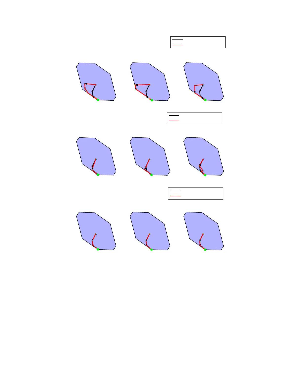
Newton Sk etc h: A Linear-time Optimization Algorithm with Linear-Quadratic Con v ergence Mert Pilanci 1 Martin J. W ain wright 1 , 2 { mert, wainwrig } @berkeley.edu Univ ersity of California, Berk eley 1 Departmen t of Electrical Engineering and Computer Science 2 Departmen t of Statistics Ma y 12, 2015 Abstract W e prop ose a randomized second-order metho d for optimization known as the New- ton Sk etc h: it is based on p erforming an appro ximate Newton step using a randomly pro jected or sub-sampled Hessian. F or self-concordant functions, w e prov e that the al- gorithm has sup er-linear con vergence with exp onen tially high probability , with conv er- gence and complexit y guarantees that are indep enden t of condition num b ers and related problem-dep enden t quantities. Given a suitable initialization, similar guaran tees also hold for strongly conv ex and smooth ob jectives without self-concordance. When implemented using randomized pro jections based on a sub-sampled Hadamard basis, the algorithm t ypically has substan tially lo w er complexit y than Newton’s metho d. W e also describ e extensions of our metho ds to programs inv olving conv ex constraints that are equipp ed with self-concordant barriers. W e discuss and illustrate applications to linear programs, quadratic programs with con v ex constraints, logistic regression and other generalized lin- ear mo dels, as well as semideﬁnite programs. 1 In tro duction Relativ e to ﬁrst-order metho ds, second-order metho ds for conv ex optimization enjoy sup erior con vergence in b oth theory and practice. F or instance, Newton’s metho d conv erges at a quadratic rate for strongly conv ex and smo oth problems, and moreov er, even for weakly con vex functions (i.e. not strongly conv ex), modiﬁcations of Newton’s method has sup er-linear con vergence compared to the m uch slow er 1 /T 2 con vergence rate that can be ac hieved b y a ﬁrst-order metho d like accelerated gradient descen t (see e.g. [15]). More imp ortan tly , at least in a uniform sense, the 1 /T 2 -rate is kno wn to b e unimprov able for ﬁrst-order metho ds [17]. Y et another issue in ﬁrst-order metho ds is the tuning of step size, whose optimal choice dep ends on the strong conv exity parameter and/or smo othness of the underlying problem. F or example, consider the problem of optimizing a function of the form x 7→ g ( Ax ), where A ∈ R n × d is a “data matrix”, and g : R n → R is a twice-diﬀeren tiable function. Here the p erformance of ﬁrst-order metho ds will dep end on b oth the con vexit y/smo othness of g , as well as the condition ing of the data matrix. In con trast, whenev er the function g is self-concordan t, then Newton’s metho d with suitably damp ed steps has a global complexity guarantee that is pro v ably indep endent of such problem-dep enden t parameters. 1 On the other hand, each step of Newton’s metho d requires solving a linear system deﬁned b y the Hessian matrix. F or instance, in application to the problem family just describ ed in volving an n × d data matrix, eac h of these steps has complexit y scaling as O ( nd 2 ). F or this reason, b oth forming the Hessian and solving the corresp onding linear system pose a tremendous numerical challenge for large v alues of ( n, d )— for instance, v alues of thousands to millions, as is common in big data applications, In order to address this issue, a multitude of diﬀeren t approximations to Newton’s method hav e b een prop osed and studied in the literature. Quasi-Newton metho ds form estimates of the Hessian by successive ev aluations of the gradien t v ectors and are computationally cheaper. Examples of such metho ds include DFP and BFGS sc hemes and also their limited memory v ersions (see the b o ok [25] for further details). A disadv an tage of suc h approximations based on ﬁrst-order information is that the associated con vergence guaran tees are t ypically m uch w eaker than those of Newton’s metho d and require stronger assumptions. Under restrictions on the eigen v alues of the Hessian (strong conv exit y and smo othness), Quasi-Newton metho ds typically exhibit lo cal sup er-linear conv ergence. In this pap er, w e prop ose and analyze a randomized approximation of Newton’s metho d, kno wn as the Newton Sketch . Instead of explicitly computing the Hessian, the Newton Sketc h metho d approximates it via a random pro jection of dimension m . When these pro jections are carried out using the randomized Hadamard transform, each iteration has complexity O ( nd log( m ) + dm 2 ). Our results sho w that it is alwa ys suﬃcient to choose m prop ortional to min { d, n } , and moreov er, that the sketc h dimension m can be m uch smaller for certain t yp es of constrained problems. Th us, in the regime n > d and with m  d , the complexity p er iteration can b e substan tially lo wer than the O ( nd 2 ) complexity of each Newton step. Sp eciﬁcally for n ≥ d 2 , the complexity of Newton Sketc h p er iteration is O ( nd log d ), which is linear in the input size ( nd ) and comparable to ﬁrst order methods whic h only access the deriv ativ e g 0 ( Ax ). Moreov er, we show that for self-concordan t functions, the total complexit y of obtaining a δ -optimal solution is O ( nd log d log(1 /δ )), and do es not dep end on constants suc h as strong conv exity or smo othness parameters unlike ﬁrst order metho ds. On the other hand, for problems with d > n , we also provide a dual strategy which eﬀectiv ely has the same guaran tees with roles of d and n exchanged. W e also consider other random pro jection matrices and sub-sampling strategies, including partial forms of random pro jection that exploit known structure in the Hessian. F or self- concordan t functions, we provide an aﬃne in v ariant analysis pro ving that the con vergence is linear-quadratic and the guarantees are indep endent of the function and data, such as condition n umbers of matrices in volv ed in the ob jective function. Finally , we describ e an in terior p oint metho d to deal with arbitrary conv ex constrain ts which combines the Newton sk etch with the barrier metho d. W e provide an upper b ound on the total n umber of iterations required to obtain a solution with a pre-sp eciﬁed target acc uracy . The remainder of this pap er is organized as follows. W e b egin in Section 2 with some bac kground on the classical form of Newton’s metho d, random matrices for sketc hing, and Gaussian widths as a measure of the size of a set. In Section 3, w e formally introduce the Newton Sketc h, including b oth fully and partially sk etc hed versions for unconstrained and constrained problems. W e pro vide some illustrative examples in Section 3.2 b efore turning to lo cal conv ergence theory in Section 3.3. Section 4 is devoted to global conv ergence results for self-concordan t functions, in both the constrained and unconstrained settings. In Section 5, w e consider a num b er of applications and pro vide additional numerical results. The bulk of our pro ofs are in given in Section 6, with some more tec hnical asp ects deferred to the app endices. 2 2 Bac kground W e b egin with some background material on the standard form of Newton’s metho d, v arious t yp es of random sk etc hes, and the notion of Gaussian width as a complexity measure. 2.1 Classical version of Newton’s metho d In this section, we brieﬂy review the con vergence prop erties and complexit y of the classical form of Newton’s metho d; see the sources [25, 4, 17] for further background. Let f : R d → R b e a closed, conv ex and t wice-diﬀeren tiable function that is b ounded b elo w. Given a con vex set C , w e assume that the constrained minimizer x ∗ : = arg min x ∈C f ( x ) (1) is uniquely deﬁned, and w e deﬁne the minim um and maxim um eigen v alues γ = λ min ( ∇ 2 f ( x ∗ )) and β = λ max ( ∇ 2 f ( x ∗ )) of the Hessian ev aluated at the minimum. W e assume moreov er that the Hessian map x 7→ ∇ 2 f ( x ) is Lipschitz con tinuous with mo dulus L , meaning that | | |∇ 2 f ( x + ∆) − ∇ 2 f ( x ) | | | op ≤ L k ∆ k 2 . (2) Under these conditions and given an initial p oint ˜ x 0 ∈ C such that k ˜ x 0 − x ∗ k 2 ≤ γ 2 L , the Newton up dates are guaranteed to conv erge quadratically—viz. k ˜ x t +1 − x ∗ k 2 ≤ 2 L γ k ˜ x t − x ∗ k 2 2 , This result is classical: for instance, see Bo yd and V andenberghe [4] for a pro of. Newton’s metho d can b e slightly mo diﬁed to b e globally con v ergent by c ho osing the step sizes via a simple bac ktrac king line-searc h pro cedure. The following result c haracterizes the complexit y of Newton’s metho d when applied to self-concordan t functions and is central in the developmen t of interior p oint metho ds (for instance, see the b o oks [18, 4]). W e defer the deﬁnitions of self-concordance and the line- searc h procedure in the follo wing sections. The num b er of iterations needed to obtain a δ appro ximate minimizer of a strictly conv ex self-concordan t function f is b ounded by 20 − 8 a ab (1 − 2 a )  f ( x 0 ) − f ( x ∗ )  + log 2 log 2 (1 /δ ) , where a, b are constan ts in the line-searc h pro cedure. 1 2.2 Diﬀeren t types of randomized sk etches V arious types of randomized sketc hes are p ossible, and we describ e a few of them here. Giv en a sketc hing matrix S ∈ R m × n , we use { s i } m i =1 to denote the collection of its n -dimensional ro ws. W e restrict our attention to sketc h matrices that are zero-mean, and that are normalized so that E [ S T S/m ] = I n . 1 T ypical v alues of these constants are a = 0 . 1 and b = 0 . 5. 3 Sub-Gaussian sketc hes: The most classical sk etch is based on a random matrix S ∈ R m × n with i.i.d. standard Gaussian en tries, or somewhat more generally , s k etch matrices based on i.i.d. sub-Gaussian ro ws. In particular, a zero-mean random vector s ∈ R n is 1-sub-Gaussian if for any u ∈ R n , w e ha v e P [ h s, u i ≥  k u k 2  ≤ e −  2 / 2 for all  ≥ 0. (3) F or instance, a vector with i.i.d. N (0 , 1) entries is 1-sub-Gaussian, as is a vector with i.i.d. Rademac her entries (uniformly distributed ov er {− 1 , +1 } ). W e use the terminology sub- Gaussian sketch to mean a random matrix S ∈ R m × n with i.i.d. rows that are zero-mean, 1-sub-Gaussian, and with cov( s ) = I n . F rom a theoretical p ersp ective, sub-Gaussian sketc hes are attractive b ecause of the w ell- kno wn concentration properties of sub-Gaussian random matrices (e.g., [5, 24]). On the other hand, from a computational p ersp ectiv e, a disadv antage of sub-Gaussian sk etches is that they require matrix-v ector m ultiplications with unstructured random matrices. In particular, giv en a data matrix A ∈ R n × d , computing its sk etched v ersion S A requires O ( mnd ) basic op erations in general (using classical matrix multiplication). Sk etches based on randomized orthonormal systems (R OS): The second type of randomized sk etc h w e consider is r andomize d orthonormal system (R OS), for which matrix m ultiplication can b e p erformed muc h more eﬃcien tly . In order to deﬁne a R OS sk etch, w e ﬁrst let H ∈ R n × n b e an orthonormal matrix with entries H ij ∈ [ − 1 √ n , 1 √ n ]. Standard classes of such matrices are the Hadamard or F ourier bases, for which matrix-vector multiplication can b e performed in O ( n log n ) time via the fast Hadamard or F ourier transforms, respectively . Based on an y suc h matrix, a sk etching matrix S ∈ R m × n from a R OS ensem ble is obtained b y sampling i.i.d. ro ws of the form s T = √ ne T j H D with probabilit y 1 /n for j = 1 , . . . , n, where the random vector e j ∈ R n is c hosen uniformly at random from the set of all n canon- ical basis vectors, and D = diag( ν ) is a diagonal matrix of i.i.d. Rademacher v ariables ν ∈ {− 1 , +1 } n . Given a fast routine for matrix-v ector multiplication, the sk etch S M for a data matrix M ∈ R n × d can be formed in O ( n d log m ) time (for instance, see the pap ers [2, 1]). Sk etches based on random row sampling: Given a probabilit y distribution { p j } n j =1 o ver [ n ] = { 1 , . . . , n } , another choice of sketc h is to randomly sample the rows of a data matrix M a total of m times with replacemen t from the given probabilit y distribution. Thus, the ro ws of S are indep endent and take on the v alues s T = e j √ p j with probabilit y p j for j = 1 , . . . , n where e j ∈ R n is the j th canonical basis vector. Diﬀeren t choices of the weigh ts { p j } n j =1 are p ossible, including those based on the row ` 2 norms p j ∝ k M e j k 2 2 and leverage v alues of M —i.e., p j ∝ k U e j k 2 for j = 1 , . . . , n , where U ∈ R n × d is the matrix of left singular vectors of M [6]. When M ∈ R n × d is the adjacency matrix of a graph with d vertices and n edges, the lev erage scores of M are also kno wn as eﬀective resistances which can b e used to sub-sample edges of a given graph by preserving its sp ectral prop erties [22]. 4 2.3 Gaussian widths In this section, w e introduce some background on the notion of Gaussian width, a wa y of measuring the size of a compact set in R d . These width measures play a k ey role in the analysis of randomized sketc hes. Given a compact subset L ⊆ R d , its Gaussian width is given b y W ( L ) : = E g  max z ∈L |h g , z i|  (4) where g ∈ R n is an i.i.d. sequence of N (0 , 1) v ariables. This complexit y measure plays an imp ortan t role in Banac h space theory , learning theory and statistics (e.g., [21, 12, 3]). Of particular interest in this pap er are sets L that are obtained by intersecting a giv en cone K with the Euclidean sphere S d − 1 = { z ∈ R n | k z k 2 = 1 } . It is easy to show that the Gaussian width of any suc h set is at most √ d , but the it can b e substan tially smaller, dep ending on the nature of the underlying cone. F or instance, if K is a subspace of dimension r < d , then a simple calculation yields that W ( K ∩ S d − 1 ) ≤ √ r . 3 Newton sk etc h and lo cal con v ergence With the basic background in place, let us now introduce the Newton sketc h algorithm, and then develop a num b er of conv ergence guaran tees associated with it. It applies to an optimization problem of the form min x ∈C f ( x ), where f : R d → R is a twice-diﬀeren tiable con vex function, and C ⊆ R d is a conv ex constrain t set. 3.1 Newton sketc h algorithm In order to motiv ate the Newton sketc h algorithm, recall the standard form of Newton’s algorithm: given a curren t iterate ˜ x t ∈ C , it generates the new iterate ˜ x t +1 b y p erforming a constrained minimization of the second order T aylor expansion—viz. ˜ x t +1 = arg min x ∈C n 1 2 h x − ˜ x t , ∇ 2 f ( ˜ x t ) ( x − ˜ x t ) i + h∇ f ( ˜ x t ) , x − ˜ x t i o . (5a) In the unconstrained case—that is, when C = R d —it tak es the simpler form ˜ x t +1 = ˜ x t −  ∇ 2 f ( ˜ x t )  − 1 ∇ f ( ˜ x t ) . (5b) No w supp ose that we hav e av ailable a Hessian matrix square ro ot ∇ 2 f ( x ) 1 / 2 —that is, a matrix ∇ 2 f ( x ) 1 / 2 of dimensions n × d such that ( ∇ 2 f ( x ) 1 / 2 ) T ∇ 2 f ( x ) 1 / 2 = ∇ 2 f ( x ) for some integer n ≥ rank( ∇ 2 f ( x )). In man y cases, suc h a matrix square ro ot can b e computed eﬃcien tly . F or instance, consider a function of the form f ( x ) = g ( Ax ) where A ∈ R n × d , and the function g : R n → R has the separable form g ( Ax ) = P n i =1 g i ( h a i , x i ). In this case, a suitable Hessian matrix square ro ot is given b y the n × d matrix ∇ 2 f ( x ) 1 / 2 : = diag  g 00 i ( h a i , x i )  n i =1 A . In Section 3.2, w e discuss v arious concrete instan tiations of suc h functions. In terms of this notation, the ordinary Newton up date can b e re-written as ˜ x t +1 = arg min x ∈C n 1 2 k∇ 2 f ( ˜ x t ) 1 / 2 ( x − ˜ x t ) k 2 2 + h∇ f ( ˜ x t ) , x − ˜ x t i | {z } ˜ Φ( x ) o , 5 and the Newton Sketc h algorithm is most easily understo o d based on this form of the up- dates. More precisely , for a sketc h dimension m to b e chosen, let S ∈ R m × n b e an isotropic sk etch matrix, satisfying the relation E [ S T S ] = I n . The Newton Sketch algorithm generates a sequence of iterates { x t } ∞ t =0 according to the recursion x t +1 : = arg min x ∈C n 1 2 k S t ∇ 2 f ( x t ) 1 / 2 ( x − x t ) k 2 2 + h∇ f ( x t ) , x − x t i | {z } Φ( x ; S t ) o , (6) where S t ∈ R m × d is an indep endent realization of a sketc hing matrix. When the problem is unconstrained, i.e., C = R d and the matrix ∇ 2 f ( x t ) 1 / 2 ( S t ) T S t ∇ 2 f ( x t ) 1 / 2 is inv ertible, the Newton sk etc h up date tak es the simpler form to x t +1 = x t −  ∇ 2 f ( x t ) 1 / 2 ( S t ) T S t ∇ 2 f ( x t ) 1 / 2  − 1 ∇ f ( x t ) . (7) The i n tuition underlying the Newton sk etch up dates is as follo ws: the iterate x t +1 corresp onds to the constrained minimizer of the random ob jective function Φ( x ; S t ) whose expectation E [Φ( x ; S t )], taking a verages ov er the isotropic sketc h matrix S t , is equal to the original Newton ob jectiv e ˜ Φ( x ). Consequen tly , it can b e seen as a sto chastic form of the Newton up date. In this pap er, we also analyze a p artial ly sketche d Newton up date , whic h tak es the following form. Giv en an additive decomp osition of the form f = f 0 + g , we p erform a sk etch of of the Hessian ∇ 2 f 0 while retaining the exact form of the Hessian ∇ 2 g . This leads to the partially sk etched up date x t +1 : = arg min x ∈C n 1 2 ( x − x t ) T Q t ( x − x t ) + h∇ f ( x t ) , x − x t i o (8) where Q t : = ( S t ∇ 2 f 0 ( x t ) 1 / 2 ) T S t ∇ 2 f 0 ( x t ) 1 / 2 + ∇ 2 g ( x t ). F or either the fully sketc hed (6) or partially sketc hed up dates (8), our analysis shows that there are man y settings in which the sk etch dimension m can b e chosen to b e substan tially smaller than n , in whic h cases the sketc hed Newton up dates will b e muc h c heap er than a standard Newton up date. F or instance, the unconstrained up date (7) can b e computed in at most O ( md 2 ) time, as opp osed to the O ( nd 2 ) time of the standard Newton up date. In constrained settings, w e sho w that the sk etch dimension m can often be c hosen even smaller— ev en m  d —whic h leads to further sa vings. 3.2 Some examples In order to provide some in tuition, let us provide some simple examples to which the sk etched Newton up dates can b e applied. Example 1 (Newton sketc h for LP solving) . Consider a linear program (LP) in the standard form min Ax ≤ b h c, x i (9) where A ∈ R n × d is a giv en constrain t matrix. W e assume that the p olytop e { x ∈ R d | Ax ≤ b } is b ounded so that the minim um achiev ed. A barrier metho d approach to this LP is based on 6 solving a sequence of problems of the form min x ∈ R d n τ h c, x i − n X i =1 log( b i − h a i , x i ) | {z } f ( x ) o , where a i ∈ R d denotes the i th ro w of A , and τ > 0 is a w eigh t parameter that is adjusted during the algorithm. By insp ection, the function f : R d → R ∪ { + ∞} is t wice-diﬀeren tiable, and its Hessian is giv en b y ∇ 2 f ( x ) = A T diag  1 ( b i −h a i , x i ) 2  A . A Hessian square ro ot is giv en b y ∇ 2 f ( x ) 1 / 2 : = diag  1 | b i −h a i , x i|  A , which allo ws us to compute a sk etc hed version of the Hessian square ro ot S ∇ 2 f ( x ) 1 / 2 = S diag  1 | b i − h a i , x i|  A. With a ROS sketc h matrix, computing this matrix requires O ( nd log( m )) basic op erations. The complexity of each Newton sketc h iteration scales as O ( md 2 ), where m is at most d . In con trast, the standard unsketc hed form of the Newton up date has complexity O ( nd 2 ), so that the sketc hed metho d is computationally cheaper whenev er there are more constraints than dimensions ( n > d ). By increasing the barrier parameter τ , we obtain a sequence of solutions that approach the optim um to the LP , which we refer to as the central path. As a simple illustration, Figure 1 compares the central paths generated by the ordinary and sk etched Newton up dates for a p olytop e deﬁned by n = 32 constrain ts in dimension d = 2. Eac h row shows three indep enden t trials of the metho d for a giv en sketc h dimension m ; the top, middle and b ottom ro ws corresp ond to sketc h dimensions m ∈ { d, 4 d, 16 d } resp ectively . Note that as the sketc h dimension m is increased, the central path tak en b y the sketc hed up dates conv erges to the standard cen tral path. As a second example, w e consider the problem of maximum likelihoo d estimation for generalized linear mo dels. Example 2 (Newton sk etc h for maximum likelihoo d estimation) . The class of generalized linear mo dels (GLMs) is used to mo del a wide v ariety of prediction and classiﬁcation problems, in which the goal is to predict some output v ariable y ∈ Y on the basis of a cov ariate vector a ∈ R d . it includes as sp ecial cases the standard linear Gaussian mo del (in which Y = R ), as w ell as logistic mo dels for classiﬁcation (in which Y = {− 1 , +1 } ), as w ell as as P oisson mo dels for coun t-v alued resp onses (in which Y = { 0 , 1 , 2 , . . . } ). See the b o ok [14] for further details and applications. Giv en a collection of n observ ations { ( y i , a i ) } n i =1 of resp onse-cov ariate pairs from some GLM, the problem of constrained maximum likelihoo d estimation b e written in the form min x ∈C n n X i =1 ψ ( h a i , x i , y i ) | {z } o , (10) where ψ : R × Y → R is a giv en con vex function, and C ⊂ R d is a con vex constrain t set, chosen b y the user to enforce a certain type of structure in the solution. Imp ortan t sp ecial cases of GLMs include the linear Gaussian mo del, in which ψ ( u, y ) = 1 2 ( y − u ) 2 , and the problem (10) 7 T rial 1 T rial 2 T rial 3 Exact Newton Newton Sketch (a) sk etc h size m = d T rial 1 T rial 2 T rial 3 Exact Newton Newton Sketch (b) sk etc h size m = 4 d T rial 1 T rial 2 T rial 3 Exact Newton Newton Sketch (c) sk etc h size m = 16 d Figure 1. Comparisons of central paths for a simple linear program in tw o dimensions. Eac h row shows three indep enden t trials for a given sk etch dimension: across the rows, the sk etc h dimension ranges as m ∈ { d, 4 d, 16 d } . The black arrows sho w Newton steps tak en by the standard in terior p oin t metho d, whereas red arrows show the steps taken by the sk etc hed v ersion. The green p oint at the vertex represents the optimum. In all cases, the sk etc hed algorithm con v erges to the optimum, and as the sketc h dimension m increases, the sk etched cen tral path conv erges to the standard central path. corresp onds to a regularized form of least-squares, as w ell as the problem of logistic regression, obtained b y setting ψ ( u, y ) = log (1 + exp( − y u )). Letting A ∈ R n × d denote the data matrix with a i ∈ R d as its i th ro w, the Hessian of the ob jectiv e (10) tak es the form ∇ 2 f ( x ) = A T diag  ψ 00 ( a T i x )  n i =1 A 8 Since the function ψ is con vex, w e are guaran teed that ψ 00 ( a T i x ) ≥ 0, and hence the quan tity diag  ψ 00 ( a T i x )  1 / 2 A can b e used as an n × d matrix square-root. W e return to explore this class of examples in more depth in Section 5.1. 3.3 Lo cal con vergence analysis using strong con vexit y Returning now to the general setting, w e now b egin by pro ving a lo cal conv ergence guarantee for the sk etched Newton up dates. In particular, this theorem provides insight in to how large the sketc h dimension m must b e in order to guarantee go o d lo cal b ehavior of the sketc hed Newton algorithm. This c hoice of sketc h dimension is determined b y geometry of the problem, in particular in terms of the tangen t cone deﬁned b y the optimum. Given a constrain t set C and the minimizer x ∗ : = arg min x ∈C f ( x ), the tangent cone at x ∗ is giv en b y K : =  ∆ ∈ R d | x ∗ + t ∆ ∈ C for some t > 0  . (11) Recalling the deﬁnition of the Gaussian width from Section 2.3, our ﬁrst main result requires the sk etc h dimension to satisfy a low er b ound of the form m ≥ c  2 max x ∈C W 2 ( ∇ 2 f ( x ) 1 / 2 K ) , (12) where  ∈ (0 , 1) is a user-deﬁned tolerance, and c is a universal constant. Since the Hessian square-ro ot ∇ 2 f ( x ) 1 / 2 has dimensions n × d , this squared Gaussian width is at at most min { n, d } . This w orst-case b ound is achiev ed for an unconstrained problem (in whic h case K = R d ), but the Gaussian width can b e substantially smaller for constrained problems. See the example following Theorem 1 for an illustration. In addition to this Gaussian width, our analysis dep ends on the cone-constrained eigen- v alues of the Hessian ∇ 2 f ( x ∗ ), whic h are deﬁned as γ = inf z ∈K∩S d − 1 h z , ∇ 2 f ( x ∗ )) z i , and β = sup z ∈K∩S d − 1 h z , ∇ 2 f ( x ∗ )) z i , (13) In the unconstrained case ( C = R d ), w e hav e K = R d , and so that γ and β reduce to the minim um and maximum eigenv alues of the Hessian ∇ 2 f ( x ∗ ). In the classical analysis of Newton’s metho d, these quantities measure the strong con vexit y and smo othness parameters of the function f . With this set-up, the follo wing theorem is applicable to any twice-diﬀeren tiable ob jective f with cone-constrained eigen v alues ( γ , β ) deﬁned in equation (13), and with Hessian that is L -Lipsc hitz con tinuous, as deﬁned in equation (2). Theorem 1 (Lo cal con v ergence of Newton Sk etch) . F or given p ar ameters δ,  ∈ (0 , 1) , c on- sider the Newton sketch up dates (6) b ase d on an initialization x 0 such that k x 0 − x ∗ k 2 ≤ δ γ 8 L , and a sketch dimension m satisfying the lower b ound (12) . Then with pr ob ability at le ast 1 − c 1 e − c 2 m , the ` 2 -err or satisﬁes the r e cursion k x t +1 − x ∗ k 2 ≤  β γ k x t − x ∗ k 2 + 4 L γ k x t − x ∗ k 2 2 . (14) The bound (14) shows that when  is set to a ﬁxed constant—sa y  = 1 / 4—the algo- rithm displa ys a linear-quadratic conv ergence rate in terms of the error ∆ t = x t − x ∗ . More 9 sp eciﬁcally , the rate is initially quadratic—that is, k ∆ t +1 k 2 ≈ 4 L γ k ∆ t k 2 2 when k ∆ t k 2 is large. Ho wev er, as the iterations progress and k ∆ t k 2 b ecomes substantially less than 1, then the rate b ecomes linear—meaning that k ∆ t +1 k 2 ≈  β γ k ∆ t k 2 —since the term 4 L γ k ∆ t k 2 2 b ecomes negligible compared to  β γ k ∆ t k 2 . If w e p erform N steps in total, the linear rate guarantees the conserv ativ e error b ounds k x N − x ∗ k 2 ≤ γ 8 L  1 2 +  β γ  N , and f ( x N ) − f ( x ∗ ) ≤ β γ 8 L  1 2 +  β γ  N . (15) A notable feature of Theorem 1 is that, dep ending on the structure of the problem, the linear-quadratic con vergence can b e obtained using a sk etc h dimension m that is substan tially smaller than min { n, d } . As an illustrative example, w e performed sim ulations for some instan- tiations of a p ortfolio optimization problem: it is a linearly-constrained quadratic program of the form min x ≥ 0 P d j =1 x j =1 n 1 2 x T A T Ax − h c, x i o , (16) where A ∈ R n × d and c ∈ R d are empirically estimated matrices and vectors (see Sec- tion 5.3 for more details). W e used the Newton sk etc h to solve diﬀerent sizes of this problem d ∈ { 10 , 20 , 30 , 40 , 50 , 60 } , and with n = d 3 in eac h case. Each problem was constructed so that the optimum x ∗ had at most s = d 2 log ( d ) e non-zero entries. A calculation of the Gaus- sian width for this problem (see App endix C for the details) sho ws that it suﬃces to tak e a sk etch dimension m % s log d , and we implemented the algorithm with this choice. Figure 2 0 2 4 6 8 10 10 −9 10 −7 10 −5 10 −3 10 −1 Log optimality gap Iteration Convergence rate of Newton Sketch n=1000 n=8000 n=27000 n=64000 n=125000 n=216000 Figure 2. Empirical illustration of the linear conv ergence of the Newton sketc h algorithm for an ensemble of p ortfolio optimization problems (16). In all cases, the algorithm w as imple- men ted using a sketc h dimension m = d 4 s log d e , where s is an upp er b ound on the num b er of non-zeros in the optimal solution x ∗ ; this quantit y satisﬁes the required low er b ound (12), and consisten t with the theory , the algorithm displa ys linear con vergence. sho ws the conv ergence rate of the Newton sketc h algorithm for the six diﬀerent problem sizes: consisten t with our theory , the sketc h dimension m  min { d, n } suﬃces to guarantee linear con vergence in all cases. It is also p ossible obtain an asymptotically sup er-linear rate b y using an iteration-dep endent sk etching accuracy  =  ( t ). The following corollary summarizes one such p ossible guarantee: 10 Corollary 1. Consider the Newton sketch iter ates using the iter ation-dep endent sketching ac cur acy  ( t ) = 1 log(1+ t ) . Then with the same pr ob ability as in The or em 1, we have k x t +1 − x ∗ k 2 ≤ 1 log(1 + t ) β γ k x t − x ∗ k 2 + 4 L γ k x t − x ∗ k 2 2 , and c onse quently, sup er-line ar c onver genc e is obtaine d—namely, lim t →∞ k x t +1 − x ∗ k 2 k x t − x ∗ k 2 = 0 . Note that the price for this sup er-linear conv ergence is that the sk etch size is inﬂated by the factor  − 2 ( t ) = log 2 (1 + t ), so it is only logarithmic in the iteration n umber. 4 Newton sk etc h for self-concordan t functions The analysis and complexity estimates given in the previous section inv olve the curv ature constan ts ( γ , β ) and the Lipsc hitz constan t L , which are seldom kno wn in practice. Moreov er, as with the analysis of classical Newton metho d, the theory is lo cal, in that the linear-quadratic con vergence tak es place once the iterates en ter a suitable basin of the origin. In this section, w e seek to obtain global conv ergence results that do not dep end on unknown problem parameters. As in the classical analysis, the appropriate setting in which to seek suc h results is for self-concordant functions, and using an appropriate form of bac ktracking line search. W e b egin by analyzing the unconstrained case, and then discuss extensions to constrained problems with self-concordan t barriers. In each case, w e show that giv en a suitable lo wer b ound on the sketc h dimension, the sketc hed Newton up dates can b e equipp ed with global conv ergence guaran tees that hold with exp onen tially high probability . Moreov er, the total num b er of iterations do es not dep end on any unknown constants suc h as strong con v exity and Lipsc hitz parameters. 4.1 Unconstrained case In this section, w e consider the unconstrained optimization problem min x ∈ R d f ( x ), where f is a closed con vex self-concordant function which is b ounded b elow. Note that a closed conv ex function φ : R → R is self-c onc or dant if | φ 000 ( x ) | ≤ 2  φ 00 ( x )  3 / 2 . (17) This deﬁnition can b e extended to a function f : R d → R b y imp osing this requirement on the univ ariate functions φ x,y ( t ) : = f ( x + ty ), for all c hoices of x, y in the domain of f . Examples of self-concordan t functions include linear and quadratic functions and negative logarithm. Self concordance is preserved under addition and aﬃne transformations. Our main result pro vide a b ound on the total n umber of Newton sk etc h iterations required to obtain a δ -accurate solution without imp osing an y sort of initialization condition (as was done in our previous analysis). This b ound scales prop ortionally to log(1 /δ ) and inv ersely in a parameter ν that dep ends on sketc hing accuracy  ∈ (0 , 1 4 ) and backtrac king parameters ( a, b ) via ν = ab η 2 1 + ( 1+  1 −  ) η where η = 1 8 1 − 1 2 ( 1+  1 −  ) 2 − a ( 1+  1 −  ) 3 . (18) 11 Algorithm 1 Unconstrained Newton Sk etc h with bac ktracking line searc h Input: Starting p oint x 0 , tolerance δ > 0, ( a, b ) line-search parameters, sketc hing matrices { S t } ∞ t =0 ∈ R m × n . 1: Compute approximate Newton step ∆ x t and approximate Newton decrement λ ( x ) ∆ x t : = arg min ∆ h∇ f ( x t ) , ∆ i + 1 2 k S t ( ∇ 2 f ( x t )) 1 / 2 ∆ k 2 2 ; e λ f ( x t ) : = ∇ f ( x ) T ∆ x t . 2: Quit if ˜ λ ( x t ) 2 / 2 ≤ δ . 3: Line search: choose µ : while f ( x t + µ ∆ x t ) > f ( x t ) + aµλ ( x t ) , µ ← bµ 4: Up date: x t +1 = x t + µ ∆ x t Output: minimizer x t , optimality gap λ ( x t ) Theorem 2. L et f b e a strictly c onvex self-c onc or dant function. Given a sketching matrix S ∈ R m × n with m ≥ c 3  2 max x ∈C rank( ∇ 2 f ( x )) = c 3  2 d , the numb er of total iter ations T for obtaining an δ appr oximate solution in function value via Algorithm 1 is b ounde d by T = f ( x 0 ) − f ( x ∗ ) ν + 0 . 65 log 2 ( 1 16 δ ) , with pr ob ability at le ast 1 − c 1 N e − c 2 m . The b ound in the ab ov e theorem sho ws that the conv ergence of the Newton Sk etc h is indep enden t of the prop erties of the function f and problem parameters, similar to classical Newton’s metho d. Note that for problems with n > d , the complexit y of each Newton sketc h step is at most O ( d 3 + nd log d ), which is smaller than that of Newton’s Metho d ( O ( nd 2 )), and also smaller than typical ﬁrst-order optimization metho ds ( O ( nd )) whenev er n > d 2 . 4.2 Newton Sketc h with self-concordant barriers W e now turn to the more general constrained case. Given a closed, conv ex self-concordant function f 0 : R d → R , let C b e a conv ex subset of R d , and consider the constrained optimization problem min x ∈C f 0 ( x ). If we are given a con v ex self-concordan t barrier function g for the constrain t set C , it is equiv alen t to consider the unconstrained problem min x ∈ R d n f 0 ( x ) + g ( x ) | {z } f ( x ) o . One w ay in which to solve this unconstrained problem is by sketc hing the Hessian of b oth f 0 and g , in which case the theory of the previous section is applicable. How ev er, there are man y cases in whic h the constraints describing C are relatively simple, and so the Hessian of g is highly-structured. F or instance, if the constraint set is the usual simplex (i.e., x ≥ 0 and h 1 , x i ≤ 1), then the Hessian of the asso ciated log barrier function is a diagonal matrix plus a rank one matrix. Other examples include problems for which g has a separable structure; suc h functions frequen tly arise as regularizers for ill-posed in verse problems. Examples of suc h regularizers include ` 2 regularization g ( x ) = 1 2 k x k 2 2 , graph regularization g ( x ) = 1 2 P i,j ∈ E ( x i − x j ) 2 induced by an edge set E (e.g., ﬁnite diﬀerences) and also other diﬀerentiable norms g ( x ) =  P d i =1 x p i  1 /p for 1 < p < ∞ . In all such cases, an attractiv e strategy is to apply a p artial Newton sketch , in which w e sk etch the Hessian term ∇ 2 f 0 ( x ) and retain the exact Hessian ∇ 2 g ( x ), as in the previously 12 describ ed updates (8). More formally , Algorithm 2 provides a summary of the steps, including the choice of the line search parameters. The main result of this section provides a guarantee on this algorithm, assuming that the sequence of sketc h dimensions { m t } ∞ t =0 is appropriately c hosen. Algorithm 2 Newton Sk etch with self-concordan t barriers Input: Starting p oint x 0 , constraint C , corresponding barrier function g suc h that f = f 0 + g , tolerance δ > 0, ( α, β ) line-search parameters, sketc hing matrices S t ∈ R m × n . 1: Compute approximate Newton step ∆ x t and approximate Newton decrement λ ( x ). ∆ x t : = arg min x t +∆ ∈C h∇ f ( x t ) , ∆ i + 1 2 k S t ( ∇ 2 f 0 ( x t )) 1 / 2 ∆ k 2 2 + 1 2 ∆ T ∇ 2 g ( x t )∆; e λ f ( x t ) : = ∇ f ( x ) T ∆ x t 2: Quit if ˜ λ ( x t ) 2 / 2 ≤ δ . 3: Line search: choose µ : while f ( x t + µ ∆ x t ) > f ( x t ) + αµλ ( x t ) , µ ← β µ . 4: Up date: x t +1 = x t + µ ∆ x t . Output: minimizer x t , optimality gap λ ( x t ). The choice of sk etch dimensions dep ends on the tangen t cones deﬁned by the iterates, namely the sets K t : =  ∆ ∈ R d | x t + α ∆ ∈ C for some α > 0  . F or a giv en sk etch accuracy  ∈ (0 , 1), we require that the sequence of sketc h dimensions satisﬁes the low er b ound m t ≥ c 3  2 max x ∈C W 2 ( ∇ 2 f ( x ) 1 / 2 K t ) . (19) Finally , the reader should recall the parameter ν w as deﬁned in equation (18), which dep ends only on the sketc hing accuracy  and the line searc h parameters. Giv en this set-up, w e hav e the follo wing guaran tee: Theorem 3. L et f : R d → R b e a c onvex and self-c onc or dant function, and let g : R d → R ∪ { + ∞} b e a c onvex and self-c onc or dant b arrier for the c onvex set C . Supp ose that we implement A lgorithm 2 with sketch dimensions { m t } t ≥ 0 satisfying the lower b ound (19) . Then taking N = f ( x 0 ) − f ( x ∗ ) ν + 0 . 65 log 2 ( 1 16 δ ) iter ations , suﬃc es to obtain δ -appr oximate solution in function value with pr ob ability at le ast 1 − c 1 N e − c 2 m . Th us, we see that the Newton Sketc h metho d can also b e used with self-concordan t barrier functions, whic h considerably extends its scop e. Section 5.5 pro vides a numerical illustration of its p erformance in this context. As we discuss in the next section, there is a ﬂexibility in c ho osing the decomp osition f 0 and g corresp onding to ob jectiv e and barrier, which enables us to also sketc h the constraints. 4.3 Sk etching with in terior p oint metho ds In this section, w e discuss the application of Newton Sk etc h to a form of barrier or interior p oin t metho ds. In particular w e discuss t wo diﬀeren t strategies and provide rigorous w orst- case complexity results when the functions in the ob jectiv e and constraints are self-concordant. 13 Algorithm 3 In terior p oint metho ds using Newton Sk etc h Input: Strictly feasible starting p oint x 0 , initial parameter τ 0 s.t. τ := τ 0 > 0, µ > 1, tolerance δ > 0. 1: Centering step: Compute b x ( τ ) by Newton Sketc h with backtrac king line-search initialized at x using Algorithm 1 or Algorithm 2. 2: Up date x := b x ( τ ). 3: Quit if r/τ ≤ δ . 4: Increase τ by τ := µτ . Output: minimizer b x ( τ ). More precisely , let us consider a problem of the form min x ∈ R d f 0 ( x ) sub ject to g j ( x ) ≤ 0 for j = 1 , . . . , r , (20) where f 0 and { g j } r j =1 are twice-diﬀeren tiable conv ex functions. W e assume that there exists a unique solution x ∗ to the ab ov e problem. The barrier metho d for computing x ∗ is based on solving a sequence of problems of the form b x ( τ ) : = arg min x ∈ R d n τ f 0 ( x ) − r X j =1 log( − g j ( x )) o , (21) for increasing v alues of the parameter τ ≥ 1. The family of solutions { b x ( τ ) } τ ≥ 1 trace out what is known as the central path. A standard b ound (e.g., [4]) on the sub-optimalit y of b x ( τ ) is giv en b y f 0 ( b x ( τ )) − f 0 ( x ∗ ) ≤ r τ . The barrier metho d successiv ely up dates the p enalt y parameter τ and also the starting p oints supplied to Newton’s metho d using previous solutions. Since Newton’s method lies at the heart of the barrier method, we can obtain a fast v ersion b y replacing the exact Newton minimization with the Newton sketc h. Algorithm 3 provides a precise description of this strategy . As noted in Step 1, there are tw o diﬀeren t strategies in dealing with the conv ex constrain ts g j ( x ) ≤ 0 for j = 1 , . . . , r : • F ul l sketch: Sketc h the full Hessian of the ob jectiv e function (21) using Algorithm 1 , • Partial sketch: Sketc h only the Hessians corresp onding to a subset of the functions { f 0 , g j , j = 1 , . . . , r } , and use exact Hessians for the other functions. Apply Algorithm 2. As shown by our theory , either approac h leads to the same con vergence guarantees, but the asso ciated computational complexity can v ary dep ending b oth on ho w data enters the ob jectiv e and constrain ts, as well as the Hessian structure arising from particular functions. The following theorem is an application of the classical results on the barrier metho d tailored for Newton Sketc h using any of the ab ov e strategies (see e.g., [4]). As b efore, the k ey parameter ν was deﬁned in Theorem 2. Theorem 4 (Newton Sketc h complexit y for in terior p oint metho ds) . F or a given tar get ac- cur acy δ ∈ (0 , 1) and any µ > 1 , the total numb er of Newton Sketch iter ations r e quir e d to obtain a δ -ac cur ate solution using Algorithm 3 is at most & log ( r / ( τ 0 δ ) log µ '  r ( µ − 1 − log µ ) γ + 0 . 65 log 2 ( 1 16 δ )  . (22) 14 If the parameter µ is set to minimize the ab o v e upper-b ound, the c hoice µ = 1 + 1 r yields O ( √ r ) iterations. How ever, when applying the standard Newton metho d, this “optimal” choice is t ypically not used in practice: instead, it is common to use a ﬁxed v alue of µ ∈ [2 , 100]. In exp erimen ts , exp erience suggests that the num b er of Newton iterations needed is a con- stan t indep enden t of r and other parameters. Theorem 4 allows us to obtain faster interior p oin t solvers with rigorous w orst-case complexity results. W e show diﬀerent applications of Algorithm 3 in the following section. 5 Applications and n umerical results In this section, w e discuss some applications of the Newton sketc h to diﬀerent optimization problems. In particular, we sho w v arious forms of Hessian structure that arise in applications, and how the Newton sk etch can b e computed. When the ob jectiv e and/or the constraints con tain more than one term, the barrier metho d with Newton Sketc h has some ﬂexibilit y in sk etching. W e discuss the choices of partial Hessian sk etc hing strategy in the barrier metho d. It is also p ossible to apply the sketc h in the primal or dual form, and w e pro vide illustrations of b oth strategies here. 5.1 Estimation in generalized linear mo dels Recall the problem of (constrained) maxim um lik eliho o d estimation for a generalized linear mo del, as previously in tro duced in Example 2. It leads to the family of optimization prob- lems (10): here ψ : R → R is a giv en conv ex function arising from the probabilistic model, and C ⊆ R d is a closed con v ex set that is used to enforce a certain t yp e of structure in the solution, P opular choices of suc h constrain ts include ` 1 -balls (for enforcin g sparsit y in a v ector), n uclear norms (for enforcing lo w-rank structure in a matrix), and other non-diﬀerentiable semi-norms based on total v ariation (e.g., P d − 1 j =1 | x j +1 − x j | ), useful for enforcing smo othness or clustering constrain ts. Supp ose that we apply the Newton sketc h algorithm to the optimization problem (10). Giv en the current iterate x t , computing the next iterate x t +1 requires solving the constrained quadratic program min x ∈C ( 1 2 k S diag  ψ 00 ( h a i , x t i , y i )  1 / 2 A ( x − x t ) k 2 2 + n X i =1 h x, ψ 0 ( h a i , x t i , y i ) i ) . (23) When the constrain t C is a scaled v ersion of the ` 1 -ball—that is, C = { x ∈ R d | k x k 1 ≤ R } for some radius R > 0—the conv ex program (23) is an instance of the Lasso program [23], for which there is a very large b o dy of w ork. F or small v alues of R , where the cardinality of the solution x is very small, an eﬀective strategy is to apply a homotop y t yp e algorithm, also kno wn as LARS [7, 9], which solves the optimality conditions starting from R = 0. F or other sets C , another p opular c hoice is pro jected gradien t descent, whic h is eﬃcient when pro jection on to C is computationally simple. F o cusing on the ` 1 -constrained case, let us consider the problem of choosing a suitable sk etch dimension m . Our choice inv olv es the ` 1 -restricted minimal eigen v alue of the data matrix A T A , whic h is given by γ − s ( A ) : = min k z k 2 =1 k z k 1 ≤ 2 √ s k Az k 2 2 . (24) 15 Note that we are alwa ys guaranteed that γ − s ( A ) ≥ λ min ( A T A ). It also inv olv es certain quan- tities that dep end on the function ψ , namely ψ 00 min : = min x ∈C min i =1 ,...,n ψ 00 ( h a i , x i , y i ) , and ψ 00 max : = max x ∈C max i =1 ,...,n ψ 00 ( h a i , x i , y i ) , where a i ∈ R d is the i th ro w of A . With this set-up, supposing that the optimal solution x ∗ has cardinality at most k x ∗ k 0 ≤ s , then it can b e sho wn (see Lemma 8 in App endix C) that it suﬃces to take a sketc h size m = c 0 ψ 00 max ψ 00 min max j =1 ,...,d k A j k 2 2 γ − s ( A ) s log d, (25) where c 0 is a universal constant. Let us consider some examples to illustrate: • Least-Squares regression: ψ ( u ) = 1 2 u 2 , ψ 00 ( u ) = 1 and ψ 00 min = ψ 00 max = 1. • Poisson regression: ψ ( u ) = e u , ψ 00 ( u ) = e u and ψ 00 max ψ 00 min = e RA max e − RA min • Logistic regression: ψ ( u ) = log (1+ e u ), ψ 00 ( u ) = e u ( e u +1) 2 and ψ 00 max ψ 00 min = e RA min e − RA max ( e − RA max +1) 2 ( e RA min +1) 2 , where A max : = max i =1 ,...,n k a i k ∞ , and A min : = min i =1 ,...,n k a i k ∞ . F or typical distributions of the data matrices, the sketc h size choice giv en in equation (25) is O ( s log d ). As an example, consider data matrices A ∈ R n × d where eac h row is indep en- den tly sampled from a sub-Gaussian distribution with v ariance 1. Then standard results on random matrices [24] show that γ − s ( A ) > 1 / 2 as long as n > c 1 s log d for a suﬃciently large constan t c 1 . In addition, we ha v e max j =1 ,...,d k A j k 2 2 = O ( n ), as w ell as ψ 00 max ψ 00 min = O (log( n )). F or suc h problems, the p er iteration complexity of Newton Sk etc h update scales as O ( s 2 d log 2 ( d )) using standard Lasso solvers (e.g., [11]) or as O ( sd log( d )) using pro jected gradient descen t. Both of these scalings are substantially smaller than conv entional algorithms that fail to exploit the small intrinsic dimension of the tangent cone. 5.2 Semideﬁnite programs The Newton sk etc h can also b e applied to semideﬁnite programs. As one illustration, let us consider the metric learning problem studied in machine learning. Given feature v ectors a 1 , . . . a n ∈ R d and corresp onding indicator y ij ∈ {− 1 , +1 } n where y ij = +1 if a i and a j b elong to the same lab el and y ij = − 1 otherwise for all i 6 = j and 1 ≤ i, j ≤ n . The task is to learn a p ositive semideﬁnite matrix X whic h represen ts a metric such that the semi-norm k a k X : = p h a, X a i establishes a nearness measure dep ending on class lab el. Using ` 2 -loss, the optimization can b e stated as the following semi-deﬁnite program (SDP) min X  0 n ( n 2 ) X i 6 = j  h X , ( a i − a j )( a i − a j ) T i − y ij  2 + λ trace( X ) o . Here the term trace( X ), along with its multiplicativ e pre-factor λ > 0 that can b e adjusted b y the user, is a regularization term for encouraging a relativ ely low-rank solution. Using 16 the standard self-concordant barrier X 7→ log det( X ) for the PSD cone, the barrier metho d in volv es solving a sequence of sub-problems of the form min X ∈ R d × d n τ n X i =1 ( h X , a i a T i i − y i ) 2 + τ λ trace X − log det ( X ) | {z } f ( vec ( X )) o . No w the Hessian of the function vec( X ) 7→ f (v ec( X )) is a d 2 × d 2 matrix giv en b y ∇ 2 f  v ec( X )  = τ ( n 2 ) X i 6 = j v ec( A ij )v ec( A ij ) T + X − 1 ⊗ X − 1 , where A ij : = ( a i − a j )( a i − a j ) T . Then we can apply the barrier metho d with partial Hessian sk etch on the ﬁrst term, { S ij v ec( A ij ) } i 6 = j and exact Hessian for the s econd term. Since the v ectorized decision v ariable is vec( X ) ∈ R d 2 the complexity of Newton Sk etc h is O ( m 2 d 2 ) while the complexity of a classical SDP interior-point solv er is O ( nd 4 ). 5.3 P ortfolio optimization and SVMs Here we consider the Marko witz formulation of the p ortfolio optimization problem [13]. The ob jectiv e is to ﬁnd x ∈ R d b elonging to the unit simplex, which corresp onds to non-negative w eights associated with eac h of d p ossible assets, so as to maximize the expected return min us a coeﬃcient times the v ariance of the return. Letting µ ∈ R d denote a v ector corresp onding to mean return of the assets, and we let Σ ∈ R d × d b e a symmetric, p ositive semideﬁnite matrix, co v ariance of the returns. The optimization problem is given by max x ≥ 0 , P d j =1 x j ≤ 1 n h µ, x i − λ x T Σ x o . (26) The co v ariance of returns is often estimated from past sto ck data via empirical cov ariance, Σ = A T A where the columns of A are time series corresp onding to assets normalized by √ n , where n is the length of the observ ation window. The barrier method can b e used solve the ab o ve problem by solving p enalized problems of the min x ∈ R d n − τ µ T x + τ λ x T A T Ax − d X i =1 log( h e i , x i ) − log(1 − h 1 , x i ) | {z } f ( x ) o , where e i ∈ R d is the i th elemen t of the canonical basis and 1 is ro w v ector of all-ones. Then the Hessian of the ab ov e barrier p enalized formulation can b e written as ∇ 2 f ( x ) = τ λ A T A + diag  x 2 i  − 1 + 11 T Consequen tly w e can sketc h the data dep endent part of the Hessian via τ λS A which has at most rank m and k eep the remaining terms in the Hessian exact. Since the matrix 11 T is rank one, the resulting sketc hed estimate is therefore diagonal plus rank ( m + 1) where the matrix in version lemma can b e applied for eﬃcient computation of the Newton Sketc h up date (see e.g. [8]). Therefore, as long as m ≤ d , the complexity p er iteration scales as O ( md 2 ), which is c heap er than the O ( nd 2 ) p er step complexit y asso ciated with classical interior point methods. W e also note that supp ort vector mac hine classiﬁcation problems with squared hinge loss also has the same form as in (26) (see e.g. [20]) where the same strategy can b e applied. 17 5.4 Unconstrained logistic regression with d  n Let us no w turn to some n umerical comparisons of the Newton Sketc h with other p opular optimization metho ds for large-scale instances of logistic regression. More sp eciﬁcally , we generated a feature matrix A ∈ R n × d based on d = 100 features and n = 16384 observ ations. Eac h row a i ∈ R d w as generated from the d -v ariate Gaussian distribution N (0 , Σ) where Σ ij = 2 | 0 . 99 | i − j . As sho wn in Figure 3, the con vergence of the algorithm p er iteration is very similar to Newton’s metho d. Besides the original Newton’s metho d, the other algorithms compared are • Gradient Descent (GD) with backtrac king line search • Accelerated Gradient Descent (Acc. GD) adapted for strongly conv ex functions with man ually tuned parameters. • Sto chastic Gradient Descent (SGD) with the classical step size choice 1 / √ t • Broyden-Fletc her-Goldfarb-Shanno algorithm (BFGS) approximating the Hessian with gradien ts. F or eac h problem, we a v eraged the p erformance of the randomized algorithms (Newton sk etc h and SGD) ov er 10 indep endent trials. W e ran the Newton sketc h algorithm with sketc h size m = 6 d . T o b e fair in comparisons, we p erformed hand-tuning of the stepsize parameters in the gradient-based metho ds so as to optimize their p erformance. The top panel in Figure 3 plots the log duality gap versus the num b er of iterations: as exp ected, on this scale, the classical form of Newton’s metho d is the fastest, whereas the SGD metho d is the slow est. Ho wev er, when the log optimality gap is plotted v ersus the w all-clo ck time in the b ottom panel, w e no w see that the Newton sketc h is the fastest. 5.5 A dual example: Lasso with d  n The regularized Lasso problem takes the form min x ∈ R d  1 2 k Ax − y k 2 2 + λ k x k 1  , where λ > 0 is a user-sp eciﬁed regularization parameter. In this section, we consider eﬃcient sketc hing strategies for this class of problems in the regime d  n . In particular, let us consider the corresp onding dual program, given by max k A T w k ∞ ≤ λ n − 1 2 k y − w k 2 2 o . By construction, the num b er of constraints d in the dual program is larger than the n umber of optimization v ariables n . If w e apply the barrier metho d to solve this dual formulation, then w e need to solve a sequence of problems of the form min w ∈ R n n τ k y − w k 2 2 − d X j =1 log( λ − h A j , w i ) − d X j =1 log( λ + h A j , w i ) | {z } f ( x ) o , where A j ∈ R n denotes the j th column of A . The Hessian of the ab ov e barrier p enalized form ulation can b e written as ∇ 2 f ( w ) = τ I n + A diag  1 ( λ − h A j , w i ) 2  A T + A diag  1 ( λ + h A j , w i ) 2  A T , 18 iterations 0 500 1000 1500 2000 2500 optimalit y gap 10 -15 10 -10 10 -5 10 0 10 5 Exact Newton GD Acc. GD SGD BFGS Newton Sketch w all-clo c k time (seconds) 0 2 4 6 8 10 12 optimalit y gap 10 -15 10 -10 10 -5 10 0 10 5 Exact Newton GD Acc. GD SGD BFGS Newton Sketch Figure 3. Newton Sk etch algorithm outp erforms other popular optimization metho ds. Plots of the log optimality gap v ersus iteration num b er (top) and plots of the log optimalit y gap versus w all-clo c k time (b ottom). Newton Sketc h empirically provides the b est accuracy in smallest w all-clo c k time, and do es not require knowledge of problem-dep endent quantities (such as strong conv exit y and smo othness parameters). Consequen tly we can k eep the ﬁrst term in the Hessian, τ I exact and apply partial sketc hing to the Hessians of the last tw o terms via S diag  1 | λ − h A j , w i| + 1 | λ + h A j , w i|  A T . Since the partially sketc hed Hessian is of the form tI n + V V T , where V is rank at most m , we can use matrix inv ersion lemma for eﬃciently calculating Newton Sk etch up dates. The complexit y of the ab ov e strategy for d > n is O ( dm 2 ), where m is at most d , whereas traditional in terior p oin t solv ers are t ypically O ( dn 2 ) p er iteration. In order to test this algorithm, w e generated a feature matrix A ∈ R n × d with d = 4096 features and n = 50 observ ations. Each row a i ∈ R d w as generated from the multiv ariate Gaussian distribution N (0 , Σ) with Σ ij = 2 ∗ | 0 . 99 | i − j . F or a given problem instance, we ran 10 indep endent trials of the sketc hed barrier metho d, and compared the results to the original barrier metho d. Figure 4 plots the the duality gap versus iteration num b er (top panel) and v ersus the wall-clock time (b ottom panel) for the original barrier metho d (blue) and sketc hed barrier metho d (red): although the sketc hed algorithm requires more iterations, these iterations are cheaper, leading to a smaller wall-clock time. This p oint is reinforced b y Figure 5, where we plot the wall-clock time required to reac h a duality gap of 10 − 6 v ersus the n umber of features n in problem families of increasing size. Note that the sketc hed barrier 19 metho d outp erforms the original barrier metho d, with signiﬁcantly less computation time for obtaining similar accuracy . 0 50 100 150 200 250 300 350 10 −10 10 −5 10 0 10 5 n u m b e r o f N e w t o n i t e r a t i o n s d u a l i t y g a p 0 2 4 6 8 10 12 14 16 18 20 10 −10 10 −5 10 0 10 5 w a l l - c l o c k t i m e ( s e c o n d s ) d u a l i t y g a p Exact Newton Newton Sketch Exact Newton Newton Sketch Figure 4. Plots of the duality gap versus iteration num b er (top panel) and duality gap versus w all-clo c k time (b ottom panel) for the original barrier metho d (blue) and sk etched barrier metho d (red). The sk etc hed interior p oint me thod is run 10 times indep endently yielding sligh tly diﬀerent curves in red. While the sketc hed metho d requires more iterations, its ov erall w all-clo c k time is m uch smaller. 6 Pro ofs W e no w turn to the pro ofs of our theorems, with more technical details deferred to the app endices. 6.1 Pro of of Theorem 1 Throughout this pro of, we let r ∈ S d − 1 denote a ﬁxed v ector that is indep endent of the sk etch matrix S t and the current iterate x t . W e then deﬁne the following pair of random v ariables Z 1 ( S ; x ) : = sup w ∈∇ 2 f ( x ) 1 / 2 K∩S n − 1 h w ,  S T S − I  r i , Z 2 ( S ; x ) : = inf w ∈∇ 2 f ( x ) 1 / 2 K∩S n − 1 k S w k 2 2 . These random v ariables are signiﬁcant, b ecause the core of our pro of is based on establishing that the error vector ∆ t = x t − x ∗ satisﬁes the recursive b ound k ∆ t +1 k 2 ≤ 6 β Z t 1 γ Z t 2 k ∆ t k 2 + 4 L γ Z t 2 k ∆ t k 2 2 , (27) 20 dimension (n) 1,000 2000 10,000 50000 100,000 wall-clock time (seconds) 0 50 100 150 200 250 300 350 400 450 500 W all-clock time for obtaining accuracy 1E-6 Exact Newton Newton Sketch Figure 5. Plot of the w all-clo c k time in seconds for reac hing a duality gap of 10 − 6 for the standard and sketc hed interior p oint metho ds as n increases (in log-scale). The sketc hed interior p oin t method has signiﬁcan tly lo wer computation time compared to the original method. where Z t 1 : = Z 1 ( S t ; x t ) and Z t 2 : = Z 2 ( S t ; x t ). W e then combine this recursion with the follo wing probabilistic guarantee on Z t 1 and Z t 2 . F or a given tolerance parameter  ∈ (0 , 1 2 ], consider the ”go o d even t” E t : =  Z t 1 ≤  2 , and Z t 2 ≥ 1 −   . (28) Lemma 1 (Suﬃcient conditions on sk etch dimension [20]) . (a) F or sub-Gaussian sketch matric es, given a sketch size m > c 0  2 max x ∈C W 2 ( ∇ 2 f ( x ) 1 / 2 K ) , we have P  E t ] ≥ 1 − c 1 e − c 2 m 2 . (29) (b) F or r andomize d ortho gonal system (ROS) sketches over the class of self-b ounding c ones, given a sketch size m > c 0 log 4 n  2 max x ∈C W 2 ( ∇ 2 f ( x ) 1 / 2 K ) , we have P  E t ] ≥ 1 − c 1 e − c 2 m 2 log 4 n . (30) Com bining Lemma 1 with the recursion (27) and re-scaling  appropriately yields the claim of the theorem. Accordingly , it remains to prov e the recursion (27), and we do so via a basic inequalit y argumen t. Recall the function x 7→ Φ( x ; S t ) that underlies the sketc h Newton up date (6): since x t and x ∗ are optimal and feasible for the constrained optimization problem, we ha v e 21 Φ( x ; S t ) ≤ Φ( x ∗ ; S t ). In tro ducing the error vector ∆ t : = x t − x ∗ , some straightforw ard algebra then then leads to the b asic ine quality 1 2 k S t ∇ 2 f ( x t ) 1 / 2 ∆ t +1 k 2 2 ≤ h S t ∇ 2 f ( x t ) 1 / 2 ∆ t +1 , S ∇ 2 f ( x t ) 1 / 2 ∆ t i − h∇ f ( x t ) − ∇ f ( x ∗ ) , ∆ t +1 i (31) Let us ﬁrst upp er bound the righ t-hand side. By using the in tegral form of T aylor’s expansion, w e ha ve h∇ f ( x t ) − ∇ f ( x ∗ ) , ∆ t +1 i = R 1 0 h∇ 2 f ( x t + u ( x ∗ − x t ))∆ t , ∆ t +1 i du , and hence RHS = Z 1 0 h h ∇ 2 f ( x t ) 1 / 2 ( S t ) T S t ∇ 2 f ( x t ) 1 / 2 − ∇ 2 f ( x t + u ( x ∗ − x t )) i ∆ t , ∆ t +1 i du By adding and subtracting terms and then applying triangle inequality , w e hav e the b ound RHS ≤ T 1 + T 2 , where T 1 : =    Z 1 0 h h ∇ 2 f ( x t ) 1 / 2  ( S t ) T S t − I  ∇ 2 f ( x t ) 1 / 2 i ∆ t , ∆ t +1 i    , and T 2 : = Z 1 0 | | |∇ 2 f ( x t + u ( x ∗ − x t )) − ∇ 2 f ( x t ) | | | op du k ∆ t k 2 k ∆ t +1 k 2 . No w observe that the vector r : = ∇ 2 f ( x t ) 1 / 2 ∆ t is indep endent of the randomness in S t , whereas the v ector ∇ 2 f ( x t ) 1 / 2 ∆ t +1 b elongs to the cone ∇ 2 f ( x t ) 1 / 2 K . Consequently , b y the deﬁnition of Z 1 , w e ha v e T 1 ≤ Z t 1 k∇ 2 f ( x t ) 1 / 2 ∆ t k 2 k∇ 2 f ( x t ) 1 / 2 ∆ t +1 k 2 . (32) No w note that using the fact that β controls the smoothness of the gradient and the Lipschitz con tinuit y of Hessian we can upp er b ound the terms on the ab ov e right-hand side as follows h ∆ t , ∇ 2 f ( x ∗ )∆ t i = h ∆ t , ∇ 2 f ( x ∗ )∆ t i + h ∆ t ,  ∇ 2 f ( x t ) − ∇ 2 f ( x ∗ )  ∆ t i ≤  β + L k ∆ t k 2  k ∆ t k 2 2 , and similarly , h ∆ t +1 , ∇ 2 f ( x ∗ )∆ t +1 i ≤  β + L k ∆ t k 2  k ∆ t +1 k 2 2 . Combining the ab ov e b ounds with (32) we obtain T 1 ≤ Z t 1  β + L k ∆ t k 2  k ∆ t +1 k 2 k ∆ t k 2 . (33) On the other hand, by the L -Lipschitz condition on the Hessian, we hav e T 2 ≤ L k ∆ t k 2 2 k ∆ t +1 k 2 . Substituting these tw o b ounds in to our basic inequality , we hav e 1 2 k S t ∇ 2 f ( x t ) 1 / 2 ∆ t +1 k 2 2 ≤ Z t 1  β + L k ∆ t k 2  k ∆ t k 2 k ∆ t +1 k 2 + L k ∆ t k 2 2 k ∆ t +1 k 2 . (34) Our ﬁnal step is to low er b ound the left-hand side (LHS) of this inequality . By deﬁnition of Z 2 , w e ha v e k S t ∇ 2 f ( x t ) 1 / 2 ∆ t +1 k 2 2 Z t 2 ≥ h ∆ t +1 , ∇ 2 f ( x t )∆ t +1 i = h ∆ t +1 , ∇ 2 f ( x ∗ )∆ t +1 i + h ∆ t +1 ,  ∇ 2 f ( x t ) − ∇ 2 f ( x ∗ )  ∆ t +1 i ≥ n γ − L k ∆ t k 2 o k ∆ t +1 k 2 2 . 22 Substituting this low er b ound into the previous inequalit y (34) and then rearranging, we ﬁnd that, as long as k ∆ t k 2 < γ 2 L , w e also hav e k ∆ t k 2 < β 2 L and consequen tly k ∆ t +1 k 2 ≤ 2 Z t 1  β + L k ∆ t k 2  Z t 2  γ − L k ∆ t k 2  k ∆ t k 2 + 2 L  γ − L k ∆ t k 2  Z t 2 k ∆ t k 2 2 ≤ 6 β Z t 1 γ Z t 2 k ∆ t k 2 + 4 L γ Z t 2 k ∆ t k 2 2 , as claimed. 6.2 Pro of of Theorem 2 Recall that in this case, we assume that f is a self-concordant strictly con v ex function. W e adopt the following notation and conv en tions from the bo ok [18]. F or a given x ∈ R d , w e deﬁne the pair of dual norms k u k x : = h∇ 2 f ( x ) u, u i 1 / 2 , and k v k ∗ x : = h∇ 2 f ( x ) − 1 v , v i 1 / 2 , as w ell as the Newton decrement λ f ( x ) = h∇ 2 f ( x ) − 1 ∇ f ( x ) , ∇ f ( x ) i 1 / 2 = k∇ 2 f ( x ) − 1 ∇ f ( x ) k x = k∇ 2 f ( x ) − 1 / 2 ∇ f ( x ) k 2 . Note that ∇ 2 f ( x ) − 1 is well-deﬁned for strictly conv ex self-concordant functions. In terms of this notation, the exact Newton up date is given by x 7→ x NE : = x + v , where v NE : = arg min z ∈C − x n 1 2 k∇ 2 f ( x ) 1 / 2 z k 2 2 + h z , ∇ f ( x ) i | {z } Φ( z ) o , (35) whereas the Newton sketc h up date is given by x 7→ x NSK : = x + v NSK , where v NSK : = arg min z ∈C − x n 1 2 k S ∇ 2 f ( x ) 1 / 2 z k 2 2 + h z , ∇ f ( x ) i o . (36) The pro of of Theorem 2 given in this section in v olves the unconstrained case ( C = R d ), whereas the pro ofs of later theorems in volv e the more general constrained case. In the unconstrained case, the tw o up dates tak e the simpler forms x NE = x − ( ∇ 2 f ( x )) − 1 ∇ f ( x ) , and x NSK = x − ( ∇ 2 f ( x ) 1 / 2 S T S ∇ 2 f ( x ) 1 / 2 ) − 1 ∇ f ( x ) . F or a self-concordan t function, the sub-optimalit y of the Newton iterate x NE in function v alue satisﬁes the b ound f ( x NE ) − min x ∈ R d f ( x ) | {z } f ( x ∗ ) ≤  λ f ( x NE )  2 . This classical b ound is not directly applicable to the Newton sk etc h up date, since it inv olves the appr oximate Newton decrement e λ f ( x ) : = −h∇ f ( x ) , v NSK i , as opp osed to the exact one λ f ( x ) : = −h∇ f ( x ) , v NE i . Th us, our strategy is to prov e that with high probability ov er the randomness in the sketc h matrix, the approximate Newton decremen t can b e used as an exit condition. Recall the deﬁnitions (35) and (36) of the exact v NE and sketc hed Newton v NSK up date directions, as well as the deﬁnition of the tangen t cone K at x ∈ C . Let K t b e the tangen t cone at x t . The follo wing lemma provides a high probability b ound on their diﬀerence: 23 Lemma 2. L et S ∈ R m × n b e a sub-Gaussian or R OS sketch matrix, and c onsider any ﬁxe d ve ctor x ∈ C indep endent of the sketch matrix. If m ≥ c 0 W ( ∇ 2 f ( x ) 1 / 2 K t ) 2  2 , then    ∇ 2 f ( x ) 1 / 2 ( v NSK − v NE )    2 ≤     ∇ 2 f ( x ) 1 / 2 v NE    2 (37) with pr ob ability at le ast 1 − c 1 e − c 2 m 2 . Similar to the standard analysis of Newton’s metho d, our analysis of the Newton sk etch algorithm is split into t wo phases deﬁned by the magnitude of the decremen t e λ f ( x ). In particular, the following lemma constitute the core of our pro of: Lemma 3. F or  ∈ (0 , 1 / 2) , ther e exist c onstants ν > 0 and η ∈ (0 , 1 / 16) such that: (a) If e λ f ( x ) > η , then f ( x NSK ) − f ( x ) ≤ − ν with pr ob ability at le ast 1 − c 1 e − c 2 m 2 . (b) Conversely, if e λ f ( x ) ≤ η , then e λ f ( x NSK ) ≤ e λ f ( x ) , and (38a) λ f ( x NSK ) ≤  16 25  λ f ( x ) , (38b) wher e b oth b ounds hold with pr ob ability 1 − c 1 e c 2 m 2 . Using this lemma, let us now complete the pro of of the theorem, dividing our analysis into the t w o phases of the algorithm. First phase analysis: By Lemma 3(a) each iteration in the ﬁrst phase decreases the func- tion v alue b y at least ν > 0, the num b er of ﬁrst phase iterations N 1 is at most N 1 : = f ( x 0 ) − f ( x ∗ ) ν , with probabilit y at least 1 − N 1 c 1 e − c 2 m . Second phase analysis: Next, let us supp ose that at some iteration t , the condition e λ f ( x t ) ≤ η holds, so that part (b) of Lemma 3 can b e applied. In fact, the b ound (38a) then guarantees that e λ f ( x t +1 ) ≤ η , so that we ma y apply the contraction b ound (38b) re- p eatedly for N 2 rounds so as to obtain that λ f ( x t + N 2 ) ≤  16 25  N 2 λ f ( x t ) with probabilit y 1 − N 2 c 1 e c 2 m . Since λ f ( x t ) ≤ η ≤ 1 / 16 by assumption, the self-concordance of f then implies that f ( x t + k ) − f ( x ∗ ) ≤  16 25  k 1 16 . Therefore, in order to ensure that and consequen tly for achieving f ( x t + k ) − f ( x ∗ ) ≤  , it suﬃces to the num b er of second phase iterations low er b ounded as N 2 ≥ 0 . 65 log 2 ( 1 16  ). 24 Putting together the tw o phases, we conclude that the total num b er of iterations N re- quired to achiev e  - accuracy is at most N = N 1 + N 2 ≤ f ( x 0 ) − f ( x ∗ ) γ + 0 . 65 log 2 ( 1 16  ) , and moreo v er, this guaran tee holds with probabilit y at least 1 − N c 1 e − c 2 m 2 . The ﬁnal step in our pro of of the theorem is to establish Lemma 3, and w e do in the next t wo subsections. 6.2.1 Pro of of Lemma 3(a) Our pro of of this part is performed conditionally on the even t D : = { e λ f ( x ) > η } . Our strategy is to sho w that the bac ktracking line search leads to a stepsize s > 0 suc h that function decremen t in moving from the current iterate x to the new sketc hed iterate x NSK = x + sv NSK is at least f ( x NSK ) − f ( x ) ≤ − ν with probability at least 1 − c 1 e − c 2 m . (39) The outline of our pro of is as follows. Deﬁning the univ ariate function g ( u ) : = f ( x + uv NSK ) and  0 = 2  1 −  , w e ﬁrst show that b u = 1 1+(1+  0 ) e λ f ( x ) satisﬁes the b ound g ( b u ) ≤ g (0) − a b u e λ f ( x ) 2 , (40a) whic h implies that b u satisﬁes the exit condition of backtrac king line search. Therefore, the stepsize s must b e low er b ounded as s ≥ b b u , which then implies that the up dated solution x NSK = x + sv NSK satisﬁes the decrement b ound f ( x NSK ) − f ( x ) ≤ − ab e λ f ( x ) 2 1 + (1 + 2  1 −  ) e λ f ( x ) . (40b) Since e λ f ( x ) > η by assumption and the function u → u 2 1+(1+ 2  1 −  ) u is monotone increasing, this b ound implies that inequality (39) holds with ν = ab η 2 1+(1+ 2  1 −  ) η . It remains to prov e the claims (40a) and (40b), for which we mak e use of the following auxiliary lemma: Lemma 4. F or u ∈ dom g ∩ R + , we have the de cr ement b ound g ( u ) ≤ g (0) + u h∇ f ( x ) , v NSK i − u k [ ∇ 2 f ( x )] 1 / 2 v NSK k 2 − log  1 − u k [ ∇ 2 f ( x )] 1 / 2 v NSK k 2  . (41) pr ovide d that u k [ ∇ 2 f ( x )] 1 / 2 v NSK k 2 < 1 . Lemma 5. With pr ob ability at le ast 1 − c 1 e − c 2 m , we have k [ ∇ 2 f ( x )] 1 / 2 v NSK k 2 2 ≤  1 +  1 −   2  e λ f ( x )  2 . (42) 25 The pro of of these lemmas are provided in App endices A.2 and A.3. Using them, let us pro ve the claims (40a) and (40b). Re calling our shorthand  0 : = 1+  1 −  − 1 = 2  1 −  , substituting inequalit y (42) into the decrement form ula (41) yields g ( u ) ≤ g (0) − u e λ f ( x ) 2 − u (1 +  0 ) e λ f ( x ) − log(1 − u (1 +  0 ) e λ f ( x )) (43) = g (0) − n u (1 +  0 ) 2 e λ f ( x ) 2 + u (1 +  0 ) e λ f ( x ) + log (1 − u (1 +  0 ) e λ f ( x )) o + u ((1 +  0 ) 2 − 1) e λ f ( x ) 2 where w e added and subtracted u (1 +  0 ) 2 e λ f ( x ) 2 so as to obtain the ﬁnal equality . W e now prov e inequality (40a). Now setting u = b u : = 1 1+(1+  0 ) e λ f ( x ) , which satisﬁes the conditions of Lemma 4 yields g ( b u ) ≤ g (0) − (1 +  0 ) e λ f ( x ) + log (1 + (1 +  0 ) e λ f ( x )) + (  0 2 + 2  0 ) e λ f ( x ) 2 1 + (1 +  0 ) e λ f ( x ) . Making use of the standard inequalit y − u + log (1 + u ) ≤ − 1 2 u 2 (1+ u ) (for instance, see the b o ok [4]), w e ﬁnd that g ( b u ) ≤ g (0) − 1 2 (1 +  0 ) 2 e λ f ( x ) 2 1 + (1 +  0 ) e λ f ( x ) + (  0 2 + 2  0 ) e λ f ( x ) 2 1 + (1 +  0 ) e λ f ( x ) = g (0) − ( 1 2 − 1 2  0 2 −  0 ) e λ f ( x ) 2 b u ≤ g (0) − α e λ f ( x ) 2 b u, where the ﬁnal inequalit y follows from our assumption α ≤ 1 2 − 1 2  0 2 −  0 . This completes the pro of of the b ound (40a). Finally , the low er b ound (40b) follows b y setting u = b b u into the decremen t inequalit y (41). 6.2.2 Pro of of Lemma 3(b) The pro of of this part hinges on the following auxiliary lemma: Lemma 6. F or al l  ∈ (0 , 1 / 2) , we have λ f ( x NSK ) ≤ (1 +  ) λ 2 f ( x ) + λ f ( x )  1 − (1 +  ) λ f ( x )  2 , and (44a) (1 −  ) λ f ( x NSK ) ≤ e λ f ( x NSK ) ≤ (1 +  ) λ f ( x NSK ) , (44b) wher e al l b ounds hold with pr ob ability at le ast 1 − c 1 e − c 2 m 2 . See App endix A.4 for the pro of. W e now use Lemma 6 to pro ve the t wo claims in the lemma statement. 26 Pro of of the b ound (38a) : Recall from the theorem statemen t that η : = 1 8 1 − 1 2 ( 1+  1 −  ) 2 − a ( 1+  1 −  ) 3 . By examining the ro ots of a p olynomial in  , it can b e seen that η ≤ 1 −  1+  1 16 . (1 +  ) λ f ( x t ) ≤ (1 +  ) e λ f ( x t ) ≤ (1 +  ) η ≤ 1 16 By applying the inequalities (44b), we hav e (1 +  ) λ f ( x ) ≤ 1 +  1 −  e λ f ( x ) ≤ 1 +  1 −  η ≤ 1 16 (45) whence inequalit y (44a) implies that λ f ( x NSK ) ≤ 1 16 λ f ( x ) + λ f ( x ) (1 − 1 16 ) 2 ≤  16 225 + 256 225   λ f ( x ) ≤ 16 25 λ f ( x ) . (46) Here the ﬁnal inequality holds for all  ∈ (0 , 1 / 2). Combining the b ound (44b) with inequal- it y (46) yields e λ f ( x NSK ) ≤ (1 +  ) λ f ( x NSK ) ≤ (1 +  )  16 25  e λ f ( x ) ≤ e λ f ( x ) , where the ﬁnal inequalit y again uses the condition  ∈ (0 , 1 2 ). This completes the pro of of the b ound (38a). Pro of of the b ound (38b) : This inequality has b een established as a consequence of proving the b ound (46). 6.3 Pro of of Theorem 3 Giv en the pro of of Theorem 2, it remains only to prov e the following mo diﬁed version of Lemma 2. It applies to the exact and sketc hed Newton directions v NE , v NSK ∈ R d that are deﬁned as follows v NE : = arg min z ∈C − x n 1 2 k∇ 2 f ( x ) 1 / 2 z k 2 2 + h z , ∇ f ( x ) i + 1 2 h z , ∇ 2 g ( x ) z i o , (47a) v NSK = arg min z ∈C − x n 1 2 k S ∇ 2 f ( x ) 1 / 2 z k 2 2 + h z , ∇ f ( x ) i + 1 2 h z , ∇ 2 g ( x ) z i | {z } Ψ( z ; S ) o . (47b) Th us, the only diﬀerence is that the Hessian ∇ 2 f ( x ) is sketc hed, whereas the term ∇ 2 g ( x ) remains unsk etc hed. Lemma 7. L et S ∈ R m × n b e a sub-Gaussian or ROS sketching matrix, and let x ∈ R d b e a (p ossibly r andom) ve ctor indep endent of S . If m ≥ c 0 max x ∈C W ( ∇ 2 f ( x ) 1 / 2 K ) 2  2 , then    ∇ 2 f ( x ) 1 / 2 ( v NSK − v NE )    2 ≤     ∇ 2 f ( x ) 1 / 2 v NE    2 (48) with pr ob ability at le ast 1 − c 1 e − c 2 m 2 . 27 7 Discussion In this pap er, w e introduced and analyzed the Newton sketc h, a randomized approximation to the classical Newton up dates. This algorithm is a natural generalization of the Itera- tiv e Hessian Sketc h (IHS) up dates analyzed in our earlier work [19]. The IHS applies only to constrained least-squares problems (for whic h the Hessian is indep endent of the iteration n umber), whereas the Newton Sk etc h applies to any an y twice diﬀerentiable function sub ject to a closed conv ex constraint set. W e describ ed v arious applications of the Newton sketc h, including its use with barrier metho ds to solve v arious forms of constrained problems. F or the minimization of self-concordant functions, the com bination of the Newton sketc h within in terior p oint up dates leads to m uch faster algorithms for an extensive b o dy of conv ex opti- mization problems. Eac h iteration of the Newton sketc h alwa ys has low er computational complexity than classical Newton’s metho d. Moreov er, it has lo wer computational complexity than ﬁrst-order metho ds when either n ≥ d 2 or d ≥ n 2 (using the dual strategy); here n and d denote the dimensions of the data matrix A . In the con text of barrier metho ds, the parameters n and d t ypically corresp ond to the num b er of constrain ts and n um b er of v ariables, resp ectiv ely . In man y “big data” problems, one of the dimensions is muc h larger than the other, in which case the Newton sketc h is adv an tageous. Moreov er, sketc hes based on the randomized Hadamard transform are well-suited to in parallel environmen ts: in this case, the sk etching step can b e done in O (log m ) time with O ( nd ) pro cessors. This scheme signiﬁcan tly decreases the amoun t of cen tral computation—namely , from O ( m 2 d + nd log m ) to O ( m 2 d + log d ). There are a n umber of op en problems associated with the Newton sk etc h. Here w e fo cused our analysis on the cases of sub-Gaussian and randomized orthogonal system (ROS) sk etches. It would also b e interesting to analyze sk etches based on co ordinate sampling, or other forms of “sparse” sketc hes (for instance, see the pap er [10]). Such techniques migh t lead to signiﬁcant gains in cases where the data matrix A is itself sparse: more sp eciﬁcally , it may b e p ossible to obtain sketc hed optimization algorithms whose computational complexity only scales with n umber of nonzero en tries in the data matrices the full dimensionalit y nd . Finally , it would b e in teresting to explore the problem of low er bounds on the sketc h dimension m . In particular, is there a threshold b elow which an y algorithm that has access only to gradients and m - sk etched Hessians must necessarily conv erge at a sub-linear rate, or in a wa y that dep ends on the strong conv exity and smo othness parameters? Such a res ult w ould clarify whether or not the guaran tees in this pap er are improv able. Ac knowledgemen ts Both authors were partially supp orted by Oﬃce of Nav al Research MURI grant N00014-11- 1-0688, and National Science F oundation Grants CIF-31712-23800 and DMS-1107000. In addition, MP was supp orted by a Microsoft Research F ello wship. A T ec hnical results for Theorem 2 In this app endix, w e collect together v arious tec hnical results and pro ofs that are required in the pro of of Theorem 2. 28 A.1 Pro of of Lemma 2 Let u b e a unit-norm vector indep endent of S , and consider the random quantities Z 1 ( S, x ) : = inf v ∈∇ 2 f ( x ) 1 / 2 K t ∩S n − 1 k S v k 2 2 and (49a) Z 2 ( S, x ) : = sup v ∈∇ 2 f ( x ) 1 / 2 K t ∩S n − 1    h u, ( S T S − I n ) v i    . (49b) By the optimality and feasibility of v NSK and v NE (resp ectiv ely) for the sketc hed Newton up date (36), we hav e 1 2 k S ∇ 2 f ( x ) 1 / 2 v NSK k 2 2 − h v NSK , ∇ f ( x ) i ≤ 1 2 k∇ 2 f ( x ) 1 / 2 v NE k 2 2 − h v NE , ∇ f ( x ) i . Deﬁning the diﬀerence vector b e : = v NSK − v NE , some algebra leads to the basic inequality 1 2 k S ∇ 2 f ( x ) 1 / 2 b e k 2 2 ≤ −h∇ 2 f ( x ) 1 / 2 v NE , S T S ∇ 2 f ( x ) 1 / 2 b e i + h b e, ∇ f ( x ) i . (50) Moreo ver, by the optimalit y and feasibility of v NE and v NSK for the exact Newton up date (35), w e ha ve h∇ 2 f ( x ) v NE − ∇ f ( x ) , b e i = h∇ 2 f ( x ) v NE − ∇ f ( x ) , v NSK − v NE i ≥ 0 . (51) Consequen tly , by adding and subtracting h∇ 2 f ( x ) v NE , b e i , w e ﬁnd that 1 2 k S ∇ 2 f ( x ) 1 / 2 b e k 2 2 ≤    h∇ 2 f ( x ) 1 / 2 v NE ,  I n − S T S  ∇ 2 f ( x ) 1 / 2 b e i    . (52) By deﬁnition, the error vector b e b elongs to the cone K t and the vector ∇ 2 f ( x ) 1 / 2 v NE is ﬁxed and indep enden t of the sketc h. Consequently , inv oking deﬁnitions (49a) and (49b) of the random v ariables Z 1 and Z 2 yields 1 2 k S ∇ 2 f ( x ) 1 / 2 b e k 2 2 ≥ Z 1 2 k∇ 2 f ( x ) 1 / 2 b e k 2 2 ,    h∇ 2 f ( x ) 1 / 2 v NE ,  I n − S T S  ∇ 2 f ( x ) 1 / 2 b e i    ≤ Z 2 k∇ 2 f ( x ) 1 / 2 v NE k 2 k∇ 2 f ( x ) 1 / 2 b e k 2 , Putting together the pieces, we ﬁnd that    ∇ 2 f ( x ) 1 / 2 ( v NSK − v NE )    2 ≤ 2 Z 2 ( S, x ) Z 1 ( S, x )    ∇ 2 f ( x ) 1 / 2 ( v NE )    2 . (53) Finally , for an y δ ∈ (0 , 1), let us deﬁne the even t E ( δ ) = { Z 1 ≥ 1 − δ, and Z 2 ≤ δ } . By Lemma 4 and Lemma 5 from our previous pap er [20], w e are guaran teed that P [ E ( δ )] ≥ 1 − c 1 e − c 2 mδ 2 . Conditioned on the even t E ( δ ), the b ound (53) implies that    ∇ 2 f ( x ) 1 / 2 ( v NSK − v NE )    2 ≤ 2 δ 1 − δ    ∇ 2 f ( x ) 1 / 2 ( v NE )    2 . By setting δ =  4 , the claim follows. 29 A.2 Pro of of Lemma 4 By construction, the function g ( u ) = f ( x + uv NSK ) is strictly conv ex and self-concordan t. Consequen tly , it satisﬁes the b ound d du  g 00 ( u ) − 1 / 2  ≤ 1, whence g 00 ( s ) − 1 / 2 − g 00 (0) − 1 / 2 = Z s 0 d du  g 00 ( u ) − 1 / 2  du ≤ s. or equiv alently g 00 ( s ) ≤ g 00 (0) (1 − sg 00 (0) 1 / 2 ) 2 for s ∈ dom g ∩ [0 , g 00 (0) − 1 / 2 ). Integrating this inequality t wice yields the b ound g ( u ) ≤ g (0) + ug 0 (0) − ug 00 (0) 1 / 2 − log(1 − ug 00 (0) 1 / 2 ) . (54) Since g 0 ( u ) = h∇ f ( x + uv NSK ) , v NSK i and g 00 ( u ) = h v NSK , ∇ 2 f ( x + uv NSK ) v NSK i , the decrement b ound (41) follo ws. A.3 Pro of of Lemma 5 W e p erform this analysis conditional on the bound (37) from Lemma 2. W e b egin b y observing that k [ ∇ 2 f ( x )] 1 / 2 v NSK k 2 ≤ k [ ∇ 2 f ( x )] 1 / 2 v NE k 2 + k [ ∇ 2 f ( x )] 1 / 2 ( v NSK − v NE ) k 2 = λ f ( x ) + k [ ∇ 2 f ( x )] 1 / 2 ( v NSK − v NE ) k 2 . (55) Lemma 2 implies that k∇ 2 [ f ( x )] 1 / 2 ( v NSK − v NE ) k 2 ≤  k∇ 2 [ f ( x )] 1 / 2 v NE k 2 = λ f ( x ). In con- junction with the b ound (56), we see that k [ ∇ 2 f ( x )] 1 / 2 v NSK k 2 ≤ (1 +  ) λ f ( x ) . (56) Our next step is to low er bound the term h∇ f ( x ) , v NSK i : in particular, b y adding and sub- tracting a factor of the original Newton step v NE , w e ﬁnd that h∇ f ( x ) , v NSK i = h [ ∇ 2 f ( x )] − 1 / 2 ∇ f ( x ) , ∇ 2 [ f ( x )] 1 / 2 v NSK i = h [ ∇ 2 f ( x )] − 1 / 2 ∇ f ( x ) , ∇ 2 [ f ( x )] 1 / 2 v NE i + h [ ∇ 2 f ( x )] − 1 / 2 ∇ f ( x ) , ∇ 2 [ f ( x )] 1 / 2 ( v NSK − v ) i = −k∇ 2 [ f ( x )] − 1 / 2 ∇ f ( x ) k 2 2 + h [ ∇ 2 f ( x )] − 1 / 2 ∇ f ( x ) , ∇ 2 [ f ( x )] 1 / 2 ( v NSK − v NE ) i ≤ −k∇ 2 [ f ( x )] − 1 / 2 ∇ f ( x ) k 2 2 + k [ ∇ 2 f ( x )] − 1 / 2 ∇ f ( x ) k 2 k∇ 2 [ f ( x )] 1 / 2 ( v NSK − v NE ) k 2 = − λ f ( x ) 2 + λ f ( x ) k∇ 2 [ f ( x )] 1 / 2 ( v NSK − v NE ) k 2 ≤ − λ f ( x ) 2 (1 −  ) , (57) where the ﬁnal step again mak es use of Lemma 2. Repeating the ab ov e argument in the rev erse direction yields the low er b ound h∇ f ( x ) , v NSK i ≥ − λ f ( x ) 2 (1 +  ), so that w e may conclude that | e λ f ( x t ) − λ f ( x t ) | ≤ λ f ( x t ) . (58) Finally , by squaring b oth sides of the inequality (56) and combining with the ab ov e b ounds giv es k [ ∇ 2 f ( x )] 1 / 2 v NSK k 2 2 ≤ − (1 +  ) 2 1 −  h∇ f ( x ) , v NSK i = (1 +  ) 2 1 −  e λ 2 f ( x ) ≤  1 +  1 −   2 e λ 2 f ( x ) , as claimed. 30 A.4 Pro of of Lemma 6 W e ha v e already prov ed the b ound (44b) during our pro of of Lemma 5—in particular, see equation (58). Accordingly , it remains only to prov e the inequality (44a). In tro ducing the shorthand e λ : = (1 +  ) λ f ( x ), w e ﬁrst claim that the Hessian satisﬁes the sandwic h relation (1 − sα ) 2 ∇ 2 f ( x )  ∇ 2 f ( x + sv NSK )  1 (1 − sα ) 2 ∇ 2 f ( x ) , (59) for | 1 − sα | < 1 where α = (1 +  ) λ f ( x ), with probability at least 1 − c 1 e − c 2 m 2 . Let us recall Theorem 4.1.6 of Nesterov [17]: it guarantees that (1 − s k v NSK k x ) 2 ∇ 2 f ( x )  ∇ 2 f ( x + sv NSK )  1 (1 − s k v NSK k x ) 2 ∇ 2 f ( x ) . (60) No w recall the b ound (37) from Lemma 2: combining it with an application of the triangle inequalit y (in terms of the semi-norm k v k x = k∇ 2 f ( x ) 1 / 2 v k 2 ) yields    ∇ 2 f ( x ) 1 / 2 v NSK    2 ≤ (1 +  )    ∇ 2 f ( x ) 1 / 2 v NE    2 = (1 +  ) k v NE k x , with probability at least 1 − e − c 1 m 2 , and substituting this inequalit y into the b ound (60) yields the sandwich relation (59) for the Hessian. Using this sandwich relation (59), the Newton decrement can b e b ounded as λ f ( x NSK ) = k∇ 2 f ( x NSK ) − 1 / 2 ∇ f ( x NSK ) k 2 ≤ 1 (1 − (1 +  ) λ f ( x )) k∇ 2 f ( x ) − 1 / 2 ∇ f ( x NSK ) k 2 = 1 (1 − (1 +  ) λ f ( x ))     ∇ 2 f ( x ) − 1 / 2  ∇ f ( x ) + Z 1 0 ∇ 2 f ( x + sv NSK ) v NSK ds      2 = 1 (1 − (1 +  ) λ f ( x ))     ∇ 2 f ( x ) − 1 / 2  ∇ f ( x ) + Z 1 0 ∇ 2 f ( x + sv NSK ) v NE ds + ∆      2 , where we hav e deﬁned ∆ = R 1 0 ∇ 2 f ( x + sv NSK ) ( v NSK − v NE ) ds . By the triangle inequality , we can write λ f ( x NSK ) ≤ 1 ( 1 − (1+  ) λ f ( x ) )  M 1 + M 2  , where M 1 : =     ∇ 2 f ( x ) − 1 / 2  ∇ f ( x ) + Z 1 0 ∇ 2 f ( x + tv NSK ) v NE dt      2 , and M 2 : =    ∇ 2 f ( x ) − 1 / 2 ∆    2 . In order to complete the pro of, it suﬃces to sho w that M 1 ≤ (1 +  ) λ f ( x ) 2 1 − (1 +  ) λ f ( x ) , and M 2 ≤ λ f ( x ) 1 − (1 +  ) λ f ( x ) . 31 Bound on M 1 : Re-arranging and then inv oking the Hessian sandwich relation (59) yields M 1 =     Z 1 0  ∇ 2 f ( x ) − 1 / 2 ∇ 2 f ( x + sv NSK ) ∇ 2 f ( x ) − 1 / 2 − I  ds  ∇ 2 f ( x ) 1 / 2 v NE      2 ≤     Z 1 0  1 (1 − s (1 +  ) λ f ( x )) 2 − 1  ds         ∇ 2 f ( x ) 1 / 2 v NE     2 = (1 +  ) λ f ( x ) 1 − (1 +  ) λ f ( x )    ∇ 2 f ( x ) 1 / 2 v NE    2 = (1 +  ) λ 2 f ( x ) 1 − (1 +  ) λ f ( x ) . Bound on M 2 : W e hav e M 2 =     Z 1 0 ∇ 2 f ( x ) − 1 / 2 ∇ 2 f ( x + sv NSK ) ∇ 2 f ( x ) − 1 / 2 ds ∇ 2 f ( x ) 1 / 2 ( v NSK − v NE )     2 ≤     Z 1 0 1 (1 − s (1 +  ) λ f ( x )) 2 ds ∇ 2 f ( x ) 1 / 2 ( v NSK − v NE )     2 = 1 1 − (1 +  ) λ f ( x )    ∇ 2 f ( x ) 1 / 2 ( v NSK − v NE )    2 ( i ) ≤ 1 1 − (1 +  ) λ f ( x )     ∇ 2 f ( x ) 1 / 2 v NE    2 = λ f ( x ) 1 − (1 +  ) λ f ( x ) , where the inequality in step (i) follows from Lemma 2. B Pro of of Lemma 7 The pro of follo ws the basic inequality argument of the pro of of Lemma 2. Since v NSK and v NE are optimal and feasible (respectively) for the sketc hed Newton problem (47b), we hav e Ψ( v NSK ; S ) ≤ Ψ( v NE ; S ). Deﬁning the diﬀerence vector b e : = v NSK − v , some algebra leads to the basic inequality 1 2 k S ∇ 2 f ( x ) 1 / 2 b e k 2 2 + 1 2 h b e, ∇ 2 g ( x ) b e i ≤ −h∇ 2 f ( x ) 1 / 2 v NE , S T S ∇ 2 f ( x ) 1 / 2 b e i + h b e,  ∇ f ( x ) − ∇ 2 g ( x )  v NE i . On the other hand since v NE and v NSK are optimal and feasible (resp ectively) for the Newton step (47a), we hav e h∇ 2 f ( x ) v NE + ∇ 2 g ( x ) v NE − ∇ f ( x ) , b e i ≥ 0 . Consequen tly , by adding and subtracting h∇ 2 f ( x ) v NE , b e i , w e ﬁnd that 1 2 k S ∇ 2 f ( x ) 1 / 2 b e k 2 2 + 1 2 h v NE , ∇ 2 g ( x ) v NE i ≤    h∇ 2 f ( x ) 1 / 2 v NE ,  I n − S T S  ∇ 2 f ( x ) 1 / 2 b e i    . By con v exity of g , we hav e ∇ 2 g ( x )  0, whence 1 2 k S ∇ 2 f ( x ) 1 / 2 b e k 2 2 ≤    h∇ 2 f ( x ) 1 / 2 v NE ,  I n − S T S  ∇ 2 f ( x ) 1 / 2 b e i    Giv en this inequalit y , the remainder of the pro of follo ws as in the pro of of Lemma 2. 32 C Gaussian widths with ` 1 -constrain ts In this app endix, w e state and prov e an elementary lemma that b ounds for the Gaussian width for a broad class of ` 1 -constrained problems. In particular, giv en a twice-diﬀeren tiable con vex function ψ , a vector c ∈ R d , a radius R and a collection of d -vectors { a i } n i =1 , consider a con v ex program of the form min x ∈C n n X i =1 ψ  h a i , x i  + h c, x i o , where C = { x ∈ R d | k x k 1 ≤ R } . (61) Lemma 8. Supp ose that the ` 1 -c onstr aine d pr o gr am (61) has a unique optimal solution x ∗ such that k x ∗ k 0 ≤ s for some inte ger s . Then denoting the tangent c one at x ∗ by K , then max x ∈C W ( ∇ 2 f ( x ) 1 / 2 K ) ≤ 6 p s log d s ψ 00 max ψ 00 min max j =1 ,...,d k A j k 2 q γ − s ( A ) , wher e ψ 00 min = min x ∈C min i =1 ,...,n ψ 00 ( h a i , x i , y i ) , and ψ 00 max = max x ∈C max i =1 ,...,n ψ 00 ( h a i , x i , y i ) . Pr o of. It is well known [16, 20] that the tangent cone of the ` 1 -norm at an y s -sparse solution is a subset of the cone { z ∈ R d | k z k 1 ≤ 2 √ s k z k 2 } . Using this fact, w e ha ve the following sequence of upp er b ounds W ( ∇ 2 f ( x ) 1 / 2 K ) = E w max z T ∇ 2 f ( x ) z =1 , z ∈K h w , ∇ 2 f ( x ) 1 / 2 z i = E w max z T A T diag ( ψ 00 ( h a i , x i x,y i )) Az =1 , z ∈K h w , diag  ψ 00 ( h a i , x i , y i )  1 / 2 Az i ≤ E w max z T A T Az ≤ 1 /ψ 00 min z ∈K h w , diag  ψ 00 ( h a i , x i , y i )  1 / 2 Az i ≤ E w max k z k 1 ≤ 2 √ s √ γ − s ( A ) 1 √ ψ 00 min h w , diag  ψ 00 ( h a i , x i , y i )  1 / 2 Az i = 2 √ s q γ − s ( A ) 1 p ψ 00 min E w k A T diag  ψ 00 ( h a i , x i , y i )  1 / 2 w k ∞ = 2 √ s q γ − s ( A ) 1 p ψ 00 min E w max j =1 ,...,d    X i =1 ,...,n w i A ij ψ 00 ( h a i , x i , y i ) 1 / 2 | {z } Q j    . Here the random v ariables Q j are zero-mean Gaussians with v ariance at most X i =1 ,...,n A 2 ij ψ 00 ( h a i , x i , y i ) ≤ ψ 00 max k A j k 2 2 . Consequen tly , applying standard b ounds on the suprema of Gaussian v ariates [12], w e obtain E w max j =1 ,...,d    X i =1 ,...,n w i A ij ψ 00 ( h a i , x i , y i ) 1 / 2    ≤ 3 p log d p ψ 00 max max j =1 ,...,d k A j k 2 . When com bined with the previous inequality , the claim follows. 33 References [1] N. Ailon and B. Chazelle. Approximate nearest neighbors and the fast Johnson- Lindenstrauss transform. In Pr o c e e dings of the thirty-eighth annual ACM symp osium on The ory of c omputing , pages 557–563. A CM, 2006. [2] N. Ailon and E. Lib erty . F ast dimension reduction using rademacher series on dual b ch co des. Discr ete Comput. Ge om , 42(4):615–630, 2009. [3] P . L. Bartlett, O. Bousquet, and S. Mendelson. Lo cal Rademacher complexities. Annals of Statistics , 33(4):1497–1537, 2005. [4] S. Boyd and L. V andenberghe. Convex optimization . Cam bridge Universit y Press, Cam- bridge, UK, 2004. [5] K. R. Da vidson and S. J. Szarek. Lo cal op erator theory , random matrices, and Banac h spaces. In Handb o ok of Banach Sp ac es , v olume 1, pages 317–336. Elsevier, Amsterdam, NL, 2001. [6] P . Drineas, M. Magdon-Ismail, M.W. Mahoney , and D.P . W o o druﬀ. F ast approximation of matrix coherence and statistical leverage. The Journal of Machine L e arning R ese ar ch , 13(1):3475–3506, 2012. [7] B. Efron, T. Hastie, I. Johnstone, and R. Tibshirani. Least angle regression. Annals of Statistics , 32(2):407–499, 2004. [8] G. Golub and C. V an Loan. Matrix Computations . Johns Hopkins Universit y Press, Baltimore, 1996. [9] T. Hastie and B. Efron. lars: Least angle regression, lasso and forward stagewise. R p ackage version 0.9-7 , 2007. [10] D.M. Kane and J. Nelson. Sparser Johnson-Lindenstrauss transforms. Journal of the A CM , 61(1):4, 2014. [11] S. Kim, K. Koh, M. Lustig, S. Boyd, and D. Gorinevsky . An in terior-p oint metho d for large-scale ` 1 -regularized least squares. IEEE Journal on Sele cte d T opics in Signal Pr o c essing , 1(4):606–617, 2007. [12] M. Ledoux and M. T alagrand. Pr ob ability in Banach Sp ac es: Isop erimetry and Pr o c esses . Springer-V erlag, New Y ork, NY, 1991. [13] H. M. Marko witz. Portfolio Sele ction . Wiley , New Y ork, 1959. [14] P . McCullagh and J.A. Nelder. Gener alize d line ar mo dels . Monographs on statistics and applied probabilit y 37. Chapman and Hall/CRC, New Y ork, 1989. [15] M. F ukushima N. Y amashita. On the rate of conv ergence of the leven b erg-marquardt metho d. In T opics in numeric al analysis , pages 239–249. Springer, 2001. [16] S. Negahban, P . Ra vikumar, M. J. W ain wrigh t, and B. Y u. A uniﬁed framew ork for high-dimensional analysis of M -estimators with decomposable regularizers. Statistic al Scienc e , 27(4):538–557, Decem b er 2012. 34 [17] Y. Nestero v. Intr o ductory L e ctur es on Convex Optimization . Klu wer Academic Publish- ers, New Y ork, 2004. [18] Y. Nestero v and A. Nemiro vski. Interior-Point Polynomial Algorithms in Convex Pr o- gr amming . SIAM Studies in Applied Mathematics, 1994. [19] M. Pilanci and M. J. W ain wright. Iterative Hessian sketc h: F ast and accurate solution appro ximation for constrained least-squares. T ec hnical rep ort, UC Berk eley , 2014. F ull length v ersion at [20] M. Pilanci and M. J. W ainwrigh t. Randomized sketc hes of conv ex programs with sharp guaran tees. T echnical rep ort, UC Berkeley , 2014. F ull length version at Presen ted in part at ISIT 2014. [21] G. Pisier. Probablistic metho ds in the geometry of Banach spaces. In Pr ob ability and A nalysis , v olume 1206 of L e ctur e Notes in Mathematics , pages 167–241. Springer, 1989. [22] D.A. Spielman and N. Sriv astav a. Graph sparsiﬁcation b y eﬀectiv e resistances. SIAM Journal on Computing , 40(6):1913–1926, 2011. [23] R. Tibshirani. Regression shrink age and selection via the Lasso. Journal of the R oyal Statistic al So ciety, Series B , 58(1):267–288, 1996. [24] R. V ershynin. Introduction to the non-asymptotic analysis of random matrices. Com- pr esse d Sensing: The ory and Applic ations , 2012. [25] S.J. W righ t and J. No cedal. Numeric al optimization , volume 2. Springer New Y ork, 1999. 35

Newton Sketch: A Linear-time Optimization Algorithm with Linear-Quadratic Convergence

Original Paper

Comments & Academic Discussion

Leave a Comment

Original Paper

Related Papers

Comments & Academic Discussion

Leave a Comment