A Group Theoretic Perspective on Unsupervised Deep Learning

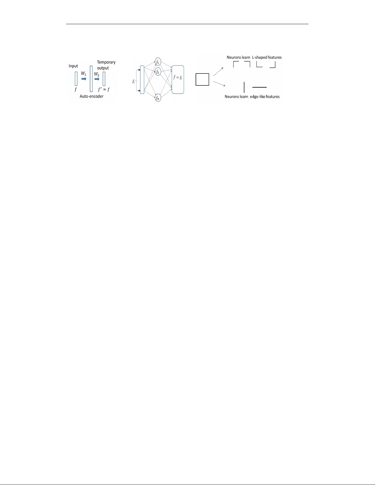
Accepted as a workshop contrib ution at ICLR 2015 A G R O U P T H E O R E T I C P E R S P E C T I V E O N U N S U P E R - V I S E D D E E P L E A R N I N G ∗ Arnab Paul Intel Corporation arnab.paul@intel.com Suresh V enkatasubramanian School of Computing, Univ ersity of Utah suresh@cs.utah.edu E X T E N D E D A B S T R A C T The modern incarnation of neural networks, now popularly known as Deep Learning (DL), accom- plished record-breaking success in processing diverse kinds of signals - vision, audio, and text. In parallel, strong interest has ensued to wards constructing a theory of DL. This paper opens up a group theory based approach, towards a theoretical understanding of DL, in particular the unsuper- vised v ariant. First we establish how a single layer of unsupervised pre-training can be e xplained in the light of orbit-stabilizer principle, and then we sketch how the same principle can be extended for multiple layers. W e focus on two key principles that (amongst others) influenced the modern DL resur gence. ( P1 ) Geoff Hinton summed this up as follows. “In order to do computer vision, first learn ho w to do computer graphics”. Hinton (2007). In other words, if a network learns a good generativ e model of its training set, then it could use the same model for classification. ( P2 ) Instead of learning an entire network all at once, learn it one layer at a time. In each round, the training layer is connected to a temporary output layer and trained to learn the weights needed to reproduce its input (i.e to solve P1 ). This step – ex ecuted layer-wise, starting with the first hidden layer and sequentially moving deeper – is often referred to as pre-training (see Hinton et al. (2006); Hinton (2007); Salakhutdinov & Hinton (2009); Bengio et al. (in preparation)) and the resulting layer is called an autoencoder . Figure 1(a) shows a schematic autoencoder . Its weight set W 1 is learnt by the netw ork. Subsequently when presented with an input f , the network will produce an output f 0 ≈ f . At this point the output units as well as the weight set W 2 are discarded. There is an alternate characterization of P1 . An autoencoder unit, such as the abov e, maps an input space to itself. Moreover , after learning, it is by definition, a stabilizer 1 of the input f . No w , input signals are often decomposable into features, and an autoencoder attempts to find a succinct set of features that all inputs can be decomposed into. Satisfying P1 means that the learned configurations can reproduce these features. Figure 1(b) illustrates this post-training behavior . If the hidden units learned features f 1 , f 2 , . . . , and one of then, say f i , comes back as input, the output must be f i . In other words learning a featur e is equivalent to searc hing for a transformation that stabilizes it . The idea of stabilizers in vites an analogy reminiscent of the orbit-stabilizer relationship studied in the theory of group actions. Suppose G is a group that acts on a set X by moving its points around (e.g groups of 2 × 2 inv ertible matrices acting ov er the Euclidean plane). Consider x ∈ X , and let O x be the set of all points reachable from x via the group action. O x is called an orbit 2 . A subset of the group elements may leave x unchanged. This subset S x (which is also a subgroup), is the stabilizer of x . If it is possible to define a notion of volume for a group, then there is an inv erse relationship ∗ This research supported in part by the NSF under grant BIGD A T A-1251049 1 A transformation T is called a stabilizer of an input f , if f 0 = T ( f ) = f . 2 The orbit O x of an element x ∈ X under the action of a group G , is defined as the set O x = { g ( x ) ∈ X | g ∈ G } . 1 Accepted as a workshop contrib ution at ICLR 2015 (a) General auto- encoder schematic (b) post-learning behavior of an auto- encoder (c) Alternate Decomposition of a Signal Figure 1: (a) W 1 is preserved, W 2 discarded (b) Post-learning, each feature is stabilized (c)Alternate ways of decomposing a signal into simpler features. The neurons could potentially learn features in the top row , or the bottom row . Almost surely , the simpler ones (bottom row) are learned. between the volumes of S x and O x , which holds ev en if x is actually a subset (as opposed to being a point). For e xample, for finite groups, the product of | O x | and | S x | is the order of the group. The inver se relationship between the volumes of orbits and stabilizers takes on a central role as we connect this back to DL. There are many possible ways to decompose signals into smaller features. Figure 1(c) illustrates this point: a rectangle can be decomposed into L-shaped features or straight- line edges. All experiments to date suggest that a neural network is likely to learn the edges. But why? T o answer this, imagine that the space of the autoencoders (viewed as transformations of the input) form a group. A batch of learning iterations stops whenever a stabilizer is found. Roughly speaking, if the search is a Markov chain (or a guided chain such as MCMC), then the bigger a stabilizer , the earlier it will be hit. The group structure implies that this big stabilizer corresponds to a small orbit. Now intuition suggests that the simpler a feature, the smaller is its orbit. For example, a line-segment generates many fe wer possible shapes under linear deformations than a flower -like shape. An autoencoder then should learn these simpler features first, which falls in line with most experiments (see Lee et al. (2009)). The intuition naturally extends to a many-layer scenario. Each hidden layer finding a feature with a big stabilizer . But beyond the first level, the inputs no longer inhabit the same space as the training samples. A “simple” feature over this new space actually corresponds to a more complex shape in the space of input samples. This process repeats as the number of layers increases. In effect, each layer learns “edge-like features” with respect to the previous layer , and from these locally simple representations we obtain the learned higher-order representation. R E F E R E N C E S Bengio, Y oshua, Goodfellow , Ian, and Courville, Aaron. Deep learning. In Deep Learning . MIT Press, in preparation. URL http://www.iro.umontreal.ca/ ~ bengioy/dlbook/ . Hinton, Geof frey E. T o recognize shapes, first learn to generate images. Pr ogr ess in brain r esear ch , 165:535–547, 2007. Hinton, Geoffre y E., Osindero, Simon, and T eh, Y ee Whye. A f ast learning algorithm for deep belief nets. Neural Computation , 18:1527–1554, 2006. Lee, Honglak, Grosse, Roger , Ranganath, Rajesh, and Ng, Andrew Y . Con volutional deep belief networks for scalable unsupervised learning of hierarchical representations. In Pr oceedings of the 26th Annual International Confer ence on Machine Learning , pp. 609–616. A CM, 2009. Salakhutdinov , Ruslan and Hinton, Geoffre y E. Deep boltzmann machines. In International Con- fer ence on Artificial Intelligence and Statistics , pp. 448–455, 2009. 2