High-performance Kernel Machines with Implicit Distributed Optimization and Randomization

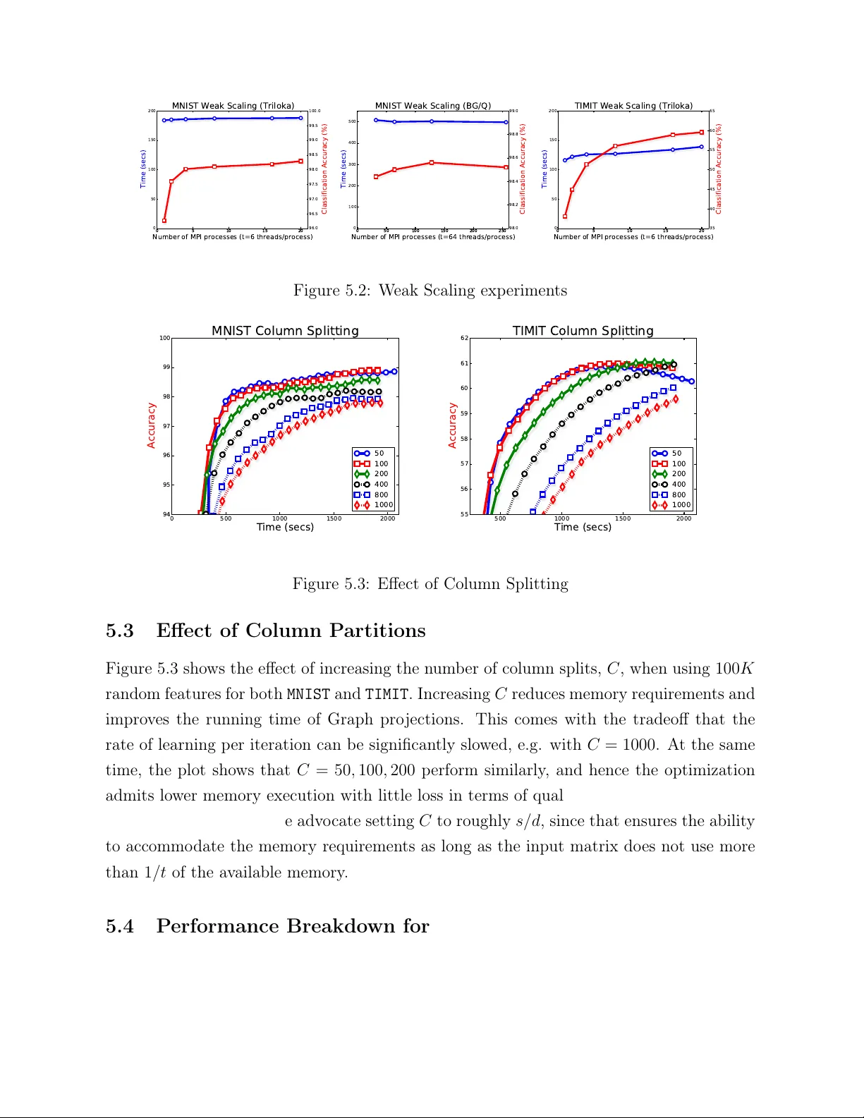
High-p erformance Kernel Mac hines with Implicit Distributed Optimization and Randomization Vik as Sindh wani ∗ Go ogle Researc h and Haim A vron IBM T.J. W atson Researc h Cen ter April 17, 2015 Abstract W e prop ose a framew ork for massiv e-scale training of k ernel-based statistical mo d- els, based on combining distributed conv ex optimization with randomization tech- niques. Our approach is based on a block-splitting v arian t of the Alternating Di- rections Method of Multipliers, carefully reconfigured to handle very large random feature matrices under memory constrain ts, while exploiting hybrid parallelism t yp- ically found in mo dern clusters of m ulticore machines. Our high-p erformance im- plemen tation supp orts a v ariety of statistical learning tasks b y enabling several loss functions, regularization sc hemes, kernels, and lay ers of randomized appro ximations for b oth dense and sparse datasets, in an extensible framew ork. W e ev aluate our implemen tation on large-scale mo del construction tasks, and provide a comparison against existing sequen tial and parallel libraries. Keywor ds: big-data, scalabilit y , k ernel methods, statistical computations ∗ The authors gratefully ac knowledge the supp ort from XD A T A program of the A dv anced Research Pro jects Agency (D ARP A), administered through Air F orce Researc h Lab oratory contract F A8750-12-C- 0323 1 1 In tro duction A large class of sup ervised machine learning mo dels are trained by solving optimization problems of the form, f ? = argmin f ∈H 1 n n X i =1 V ( y i , f ( x i )) + λr ( f ) , (1.1) where, • { ( x i , y i ) } n i =1 is a training set with n lab eled examples, with inputs x ∈ X ⊂ R d and asso ciated target outputs y ∈ Y ⊂ R m ; • H is a hypothesis space of functions mapping the input domain (a subset of R d ) to the output domain (another subset of R m ), ov er which the training pro cess estimates a functional dependency f ? ( · ) b y optimizing an ob jective function; • V ( · , · ) in a con v ex loss function which measures the discrepancy b etw een “ground truth" and model prediction; • r ( · ) is a con vex regularizer that p enalizes mo dels according to their complexit y , in order to prev en t ov erfitting. The regularization parameter λ balances the classic tradeoff b et w een data fitting and complexit y con trol, whic h enables generalization to unseen test data. One prev alent setting is that of a large training set (big n ), with high-dimensional inputs and outputs. In suc h a setting, it is often relativ ely easier to solv e (1.1) if w e imp ose strong structural constrain ts on the mo del, e.g. b y requiring H to b e linear, or severely restricted it in terms of sparsit y or smo othness. How ever, it is now w ell appreciated among practitioners, that imp osing suc h strong structural constrain ts on the mo del upfron t often limits, b oth theoretically and empirically , the p oten tial of big data in terms of delivering higher accuracy mo dels. When strong constraints are imposed, data tends to exhausts the statistical capacit y of the mo del causing generalization p erformance to quic kly saturate. As a consequence, practitioners are increasingly turning to highly nonlinear models with millions of parameters, or ev en infinite-dimensional mo dels, that need to b e estimated on v ery large datasets (see Hinton et al. (2012); T aigman et al. (2014); Krizhevsky et al. (2012); So c her et al. (2013); Huang et al. (2014)), often with carefully designed domain- dep enden t loss functions and regularizers. This trend, exemplified b y the recent success of deep learning tec hniques, necessitates co-design at the intersection of statistics, numerical optimization and high p erformance computing. Indeed, highly scalable algorithms and implemen tations pla y a piv otal role in this setting as enablers of rapid exp erimentation of statistical tec hniques on massiv e datasets to gain b etter understanding of their ability to 2 truly utilize "big data", which, in turn, informs the design of even more effective statistical algorithms. Kernel metho ds (see Sc hlkopf and Smola (2001)) constitute a mathematically elegant framew ork for general-purp ose infinite-dimensional non-parametric statistical inference. By providing a principled framework to extend classical linear statistical tec hniques to non-parametric mo deling, their applications span the en tire sp ectrum of statistical learn- ing: nonlinear classification, regression, clustering, time-series analysis, sequence mo del- ing (Song et al. (2013)), dynamical systems (Bo ots et al. (2013)), hypothesis testing (Har- c haoui et al. (2013)), causal mo deling (Zhang et al. (2011)) and others. The cen tral ob ject in k ernel metho ds is a k ernel function k ( x , x 0 ) defined on the input domain X . This k ernel function defines a suitable hypothesis space of functions H k with whic h (1.1) can be instan tiated, and turned into a finite dimensional optimization problem. Ho w ever, training pro cedures deriv ed directly in this manner scale p o orly , having training time that is cubic in n and storage that is quadratic in n , with limited opp ortunities for parallelization. This p o or scalability p oses a significant barrier for the use of kernel metho ds in big data applications. As such, with the gro wth in data across a multitude of applications, scaling up k ernel metho ds Bottou et al. (2007) has acquired renewed and somewhat urgen t significance. In this w ork, w e dev elop a highly scalable algorithmic framework and softw are im- plemen tation for kernel metho ds, for distributed-memory computing environmen ts. Our framew ork com bines tw o recent algorithmic tec hniques: randomized feature maps and dis- tributed optimization metho d based on the Alternating Directions Metho d of Multipliers (ADMM) describ ed b y Boyd et al. (2011). This framework orchestrates lo cal mo dels es- timated on a subset of examples and random features, tow ards a unified solution. Our approac h builds on the blo ck-splitting ADMM framew ork proposed by Parikh and Bo yd (2014), but we carefully reorganize its up date rules to extract muc h greater efficiency . Our framew ork is designed to b e highly mo d ular. In particular, one needs to only supply cer- tain proximal op erators asso ciated with a custom loss function and the regularizer. Our ADMM wrapp er can then immediately instantiate a solver for (1.1) for a v ariety of choices of k ernels and learning tasks. W e b enc hmark our implementation in b oth high-p erformance computing environmen ts as w ell as commo dit y clusters. Results indicate that our approac h is highly scalable in b oth settings, and is capable of returning state-of-the-art p erformance in machine learning tasks. Comparisons against sequential and parallel libraries for Supp ort V ector Mac hines sho ws highly fav orable accuracy-time tradeoffs for our approach. 3 W e ackno wledge that the tw o main tec hnical ingredients (namely , randomized feature maps and blo ck splitting ADMM) of our pap er are b oth based on kno wn influential tec h- niques. Ho wev er, their combination in our framew ork is entirely nov el and motiv ated by our empirical observ ations on real-world problems where it b ecame eviden t that a care- fully customized distributed solv er was necessary to push the random features technique to its limits. By using a blo c k splitting ADMM strategy on an implicitly defined (and partitioned) feature-map expanded matrix, whic h is rep eatedly computed on the fly , w e are able to control memory consumption and handle extremely large data dense matrices that arise due to b oth v ery large n um b er of examples as well as random features. W e stress that our com bination requires mo difying the blo ck-splitting ADMM iterations in order to a void memory consumption from b ecoming excessiv e v ery quic kly . As w e sho w in the experimental section, this leads to a scalable solver that b ears fruit empirically . The co de is freely a v ailable for do wnload and use as part of the libSkylark library( http: //xdata- skylark.github.io/libskylark/ ). The rest of this article is organized as follo ws. In section 2 we pro vide a brief bac kground on v arious tec hnical elements of our algorithm. In section 3 we describ e the prop osed algo- rithm. In section 4 w e discuss the role of the random feature transforms in our algorithm. In section 5 w e rep ort experimental results on t wo widely used machine learning datasets: MNIST (image classification) and TIMIT (sp eech recognition). W e finish with some conclu- sions in section 6. 2 T ec hnical Bac kground In this section w e provide a brief background on v arious technical elements of our algorithm. 2.1 Kernel Metho ds and Their Scalability Problem W e start with a brief description of k ernel methods. A kernel function, k : X × X 7→ R , is defined on the input domain X ⊂ R d . This k ernel function implicitly defines a hypothesis space of functions – the Repro ducing Kernel Hilbert Space H k . The h yp othesis space H k is also equipp ed with a norm k · k k whic h acts as a natural candidate for the regularizer, i.e. r ( f ) = k f k 2 k . H k is then used to instan tiate the learning problem (1.1) with H = H k . The attractiv eness of using H k as the h yp othesis space in (1.1) stems from the Represen- ter Theorem (see W ah ba (1990)), which guarantees that the solution admits the follo wing 4 expansion (for each co ordinate f j ( · ) of the v ector v alued function f ? ( · ) in (1.1)), f ? j ( x ) = n X i =1 α j i k ( x , x i ) , j = 1 . . . m . (2.1) The expansion (2.1) is then used to turn (1.1) to a finite dimensional optimization problem, whic h can b e solv ed n umerically . Consider, for example, the solution of (1.1) for the square loss ob jectiv e V ( y , y ) = k y − t k 2 2 . Plugging the expansion (2.1) in to (1.1), the co efficients α ij , j = 1 . . . m, i = 1 . . . , n can be found b y solving the following linear system, ( K + nλ I n ) α = Y , (2.2) where Y ∈ R n × m with row i equal to y i , K is the n × n Gram matrix giv en b y K ij = k ( x i , x j ) , and α ∈ R n × m con tains the co efficien ts α ij . Problem (1.1) with other loss func- tions ( V ( · , · ) ), and “kernelization" of other linear statistical learning algorithms giv es rise to a whole suite of statistical mo deling tec hniques. F or a suitable choices of a k ernels, the hypothesis space H k can b e made very ric h, th us implying very strong non-parameteric mo deling capabilities, while still allowing the solution of (1.1) via n umerical optimization. Ho wev er, there is a steep price in terms of scalabilit y . Consider, again, the solution of (1.1) for the squared loss. As K is t ypically dense, solving (2.2) using a direct metho d incurs a Θ ( n 3 + n 2 ( d + m )) time complexit y , and Θ( n 2 ) storage complexit y . Once α is found, ev aluating f ? ( · ) on new data p oin t requires Θ ( n ( d + m )) . This training and test time complexity becomes unapp ealing wh en n is large. 2.2 Randomized Kernel Metho ds Randomized kernel metho ds, pioneered b y Rahimi and Rech t (2007), has recen tly emerged as a key algorithmic device with which to dramatically accelerate the training of k ernel metho ds via a linearization mec hanism. T o help understand the b enefits of linearization, let us first compare the complexit y of k ernel metho ds on the square loss function, to the complexit y of solving (1.1) in a linear h yp othesis space H l = { f W : W ∈ R d × m , f W ( x ) = W T x } . 5 With H = H l , problem (1.1) reduces to solving the follo wing ridge regression problem W ? = argmin W ∈ R d × m 1 n k XW − Y k 2 f ro + λ k W k 2 f ro , where X ∈ R n × d has row i equal to x i . Using classical direct metho ds, this problem can b e solv ed in Θ( nd 2 + ndm + d 2 m ) op erations, using Θ( nd ) memory and requiring only Θ( dm ) for ev aluating f ? ( · ) . The linear dep endence on n (the “big” dimension) is m uc h more attractiv e for large-scale problems. F urthermore, recently Demmel et al. (2012) show ed that distributed implemen tations of k ey linear algebra k ernels can b e made comm unication efficien t; w e also note that the running time can b e improv ed by using more modern algorithms based on randomized preconditioning (see A vron et al. (2010); Meng et al. (2014)). Thus, while H l is a weak er hypothesis space from a statistical mo deling p oin t of view, is muc h more attractive from a computational p oint of view. Randomized kernel metho ds linearize H k b y constructing an explicit feature mapping z : R d 7→ R s suc h that k ( x , y ) ≈ z ( x ) T z ( y ) . W e now solv e (1.1) on H k,l instead of H k , where H k,l = { f W : W ∈ R s × m , f W ( x ) = W T z ( x ) } . This is a linear regression problem that can be solv ed more efficien tly . In particular, returning to the previous example with squared loss and regularizer r ( f W ) = k W k 2 f ro , the problem reduces to solving W ? = argmin W ∈ R s × t 1 n k ZW − Y k 2 f ro + λ k W k 2 f ro , where Z ∈ R n × s has ro w i equal to z ( x i ) . In general form, after selecting some z ( · ) (a c hoice that is guided by the kernel k ( · , · ) w e w ant to use), we are faced with solving the problem argmin W ∈ R s × m 1 n n X i =1 V  y i , W T z i  + λr ( W ) (2.3) where z i = z ( x i ) . This technique relies on ha ving a go o d appro ximation to k ( · , · ) with mo derate sizes of s , and ha ving a cheap mechanism to generate the random feature matrix Z from X . Randomized feature maps ha ve pro ven to b e very effectiv e in extending the reac h of k ernel methods to larger datasets, e.g. on classical sp eec h recognition datasets Huang et al. (2014). Ho w ev er, it has also b een observed that in order to build state-of-the-art mo dels 6 1 0 2 1 0 3 1 0 4 1 0 5 Number of Random Features 0 20 40 60 80 100 Accuracy Classification Accuracy on TIMIT Accuracy state of the art 1 0 2 1 0 3 1 0 4 1 0 5 0 1000 2000 3000 4000 5000 6000 7000 8000 9000 Memory Requirements (GB) Memory (GB) Figure 2.1: P erformance of Randomized Kernel Metho ds. The largest mo del is trained on a sup ercomputer (BlueGene/Q), on an 8 . 7 terab yte dataset using implicit distributed optimization metho ds implemen ted in this pap er for high-p erformance computing environ- men ts. in applications of interest, a v ery large num b er of random features are needed (very large s ). This is illustrated in Figure 2.1, whic h examines the use of (2.3) in a sp eech recognition application. This large num b er of features is c hallenging from a n umerical optimization p oin t of view. F or example, the transformed data matrix Z (whose rows are z ( x i ) ) no w requires several terab ytes of data, even though the original data matrix X do es not require to o m uch storage. 2.3 Distributed Con v ex Optimization with ADMM This section reviews distributed optimization using v ariants of the Alternating Direction Metho d of Multipliers (ADMM) described b y Bo yd et al. (2011). Informally speaking, one ma y tak e the follo wing heuristic approac h for building statisti- cal mo dels using big datasets on distributed memory compute en vironments: partition the data b et ween no des, build a lo cal mo dels in each no de, and generate a global mo del using some com bination mechanism (e.g. av eraging o v er the ensem ble of lo cal mo dels). ADMM as applied to statistical learning problems follows a similar pattern, in that it orchestrates the estimation of the lo cal mo dels in the presence of a global mo del as prior. The app eal of ADMM is that it decomp oses the problem in to a set of proximal and pro jection op erators whic h are computational patterns that rep eat across a v ariety of settings. Thus, ADMM can b e seen as a meta-algorithm, in which the user needs to only implement a small set of operators required to instan tiate their problem, and ADMM as a wrapp er takes care of 7 distributing the computation. More concretely , ADMM solv es optimization problems of the general form, argmin x ∈ R n , z ∈ R m f ( x ) + g ( z ) sub ject to : Ax + Bz = c (2.4) In this form, the ob jective function splits ov er con v ex functions f , g in volving separate v ariables, tied via a linear constraint where A ∈ R p × n , B ∈ R p × m , c ∈ R p . ADMM up date rules are derived via Gauss-Seidel up dates (cyclic coordinate descent) on the augmen ted Lagrangian, L ρ ( x , z , ˜ ν ) = f ( x ) + g ( z ) + ˜ ν T ( Ax + Bz − c ) + ρ 2 k Ax + Bz − c k 2 2 , resulting in the follo wing iterations, x ( j +1) = argmin x ∈ R n L ρ ( x , z ( j ) , ˜ ν ( j ) ) (2.5) z ( j +1) = argmin z ∈ R m L ρ ( x ( j +1) , z , ˜ ν ( j ) ) (2.6) ˜ ν ( j +1) = ˜ ν ( j ) + ρ  Ax ( j +1) + Bz ( j +1) − c  (2.7) where ρ > 0 is the ADMM p enalt y parameter and ˜ ν are dual v ariables asso ciated with the constrain t. A generic constrained con v ex optimization problem, argmin x ∈ R d f ( x ) sub ject to x ∈ C (2.8) can be cast in ADMM form as, argmin x , z f ( x ) + I C ( z ) sub ject to x = z , (2.9) where I C ( z ) is 0 if z ∈ C and + ∞ otherwise. Ab o ve, the ob jective function and the constrain t are separated b y v ariable splitting and a consensus constrain t is added. The augmen ted Lagrangian for this problem is giv en by , L ρ ( x , z , ν ) = f ( x ) + I C ( z ) + ˜ ν T ( x − z ) + ρ 2 k x − z k 2 2 . 8 Th us, the ADMM up date equations for solving (2.9) are x ( j +1) = argmin x ∈ R n h f ( x ) + x T ˜ ν ( j ) + ρ 2 k x − z ( j ) k 2 2 i = argmin x ∈ R n   1 ρ f ( x ) + 1 2      x − z ( j ) − ˜ ν ( j ) ρ !      2 2   z ( j +1) = argmin z ∈ R m   I C ( z ) + ρ 2      z − x ( j +1) + ˜ ν ( j ) ρ !      2 2   ˜ ν ( j +1) = ˜ ν ( j ) + ρ  x ( j +1) − z ( j +1)  In order to rewrite these equations more compactly , it is useful to define the following op erators. Definition 1 (Proximit y Op erator) The Pr oximity (or Pr ox) op er ator asso ciate d with a function f : R d 7→ R is a map prox f : R d 7→ R d given by prox f [ x ] = argmin y ∈ R d 1 2 k x − y k 2 2 + f ( y ) Definition 2 (Pro jection Op erator) The Pr oje ction op er ator asso ciate d with a c onvex c onstr aint set C is the map proj C : R d 7→ R d given by proj C [ x ] = argmin y ∈C 1 2 k x − y k 2 2 Henc e, proj C = prox I C . F or a v ariet y of common loss functions and regularizers, th e pro ximal op erator admits closed-form form ulas, that can b e computed using efficient algorithms. In addition, w e use the sc ale d dual variables ν ( j ) ≡ ρ − 1 ˜ ν ( j ) . T ogether with the ab ov e w e get the follo wing up date rules: x ( j +1) = prox 1 ρ f [ z ( j ) − ν ( j ) ] z ( j +1) = proj C [ x ( j +1) + ν ( j )] (2.10) ν ( j +1) = ν ( j ) + x ( j +1) − z ( j +1) 9 3 Distributed Learning with ADMM Blo c k Splitting and Hybrid P arallelism In this section w e describ e the prop osed algorithm for solving (2.3). Psuedo-code is given as Algorithm 1. In the following, the matrix X , Y are the input of the algorithm, where X has x i as row i , and Y i has y i as row i . The matrix Z denotes the result of applying the random transform z ( · ) to X , that is ro w i of Z is z ( x i ) . Our algorithm is geared to wards the follo wing setup: • A distributed-memory computing environmen t comprising of a cluster of N compute no des, with T cores p er no de. W e assume that each no de has M GB of RAM. • The training data X , Y are distributed by r ows across the no des. This is a natural assumption in large-scale learning since ro ws hav e the semantics of data instances whic h are typically collected or generated in parallel across the cluster to b egin with. • X , Y fit in the aggregate distributed memory of the cluster, but are large enough that they cannot fit on a single no de, and cannot b e replicated in memory on multiple no des. • The matrix Z do es not fit in aggregate distributed memory b ecause n and s are b oth sim ultaneously big. This assumption is motiv ated b y empirical observ ations sho wn in Figure 2.1. • The matrix Z cannot b e stored on disk b ecause of space restrictions, or it can but the I/O cost of reading it by blocks in ev ery iteration is more exp ensiv e than the cost of recomputing blo cks of Z on the fly from scratch as needed , resp ecting p er-no de memory constraints. Thus, our algorithm uses a transform op erator T whic h when applied to X i giv en a blo ck id j , produces the output Z ij , i.e., T [ X i , j ] = Z ij This transform function is used to generate Z ij as needed in the optimization pro cess, used and discarded in eac h iteration. The construction of these transform operators is discussed in Section 4. Our algorithm is based on the block-splitting v ariant of ADMM describ ed by Parikh and Bo yd (2014), which is w ell suited for the target setup. This approac h assumes the data matrix is partitioned b y b oth ro ws and columns. Indep endent mo dels are estimated on 10 eac h blo c k in parallel and orc hestrated b y ADMM tow ards the solution of the optimization problem. In addition to the pro ximal and pro jection op erators, this v arian t mak es use of the follo wing op erator. Definition 3 (Graph Pro jection Op erator Ov er Matrices) The Gr aph pr oje ction op- er ator asso ciate d with an n × d matrix A is the map proj A : R n × k × R d × k 7→ R n × k × R d × k given by, proj A [( Y , X )] = argmin ( V , U ) 1 2 k V − Y k 2 f ro + 1 2 k U − X k 2 f ro , subje ct to : V = AU wher e Y , V ∈ R n × k , X , U ∈ R d × k . The solution is given by: U = [ A T A + I ] − 1 ( X + A T Y ) (3.1) V = A U (3.2) Remark The abov e solution formula is computationally preferable when d  n . When d is larger, the solution formula may b e rewritten in terms of an n × n linear system in v olving AA T instead (see Parikh and Boyd (2014)). How ever, the d  n case is more relev an t for our setting. Our algorithm is derived b y first logically blo ck partitioning the matrix Z into R × C blo c ks, where R and C denote row and column splitting parameters resp ectively . The matrices X and Y are ro w partitioned in to R blo c ks, while W is row partitioned in to C blo c ks:     X 1 . . . X R     → . . . →       Z 11 Z 12 . . . Z 1 C . . . . . . . . . . . . Z R 1 Z R 2 . . . Z RC       ,     Y 1 . . . Y R     ,     W 1 . . . W C     (3.3) W e assume that X i ∈ R n i × m , Y i ∈ R n i × m , W j ∈ R s j × m , Z ij ∈ R n i × s j where P R i =1 n i = n and P C j =1 s j = s . W e assume a distributed-memory setup in whic h R pro cesses are in v ok ed on N ≤ R no des, with the pro cesses distributed ev enly among the no des. Pro cesses communicate using message-passing; in our implemen tation, using the MPI (Message Passing Interface) proto col. Eac h pro cess o wns a row index i , i.e. it holds in memory X i and Y i . In the notation, w e use i as an iden tifier of the pro cess. W e assume process i spa wns t ≤ T threads 11 that collectiv ely o wn the parallel computation related to the C blo cks of Z ij , j = 1 . . . C . Setting the v alues of t , R and C are configuration options of the algorithm, how ever it should alw a ys b e the case that t × R ≤ N × T , and it is advisable that t ≤ C . F or reasoning ab out the algorithm, it is useful to assume that n is a m ultiple of R and that s is a multiple of C , and that w e set n i = n R and s j = s C . In practice, n and s are usually not exact m ultiples of R and C , and there is an imbalance in the v alues of { n i } and { s j } . T o in terpret the blo ck-splitting ADMM algorithm, it is con venien t to setup the follo wing seman tics. Let W ij ∈ R s j × m denote lo cal mo del parameters asso ciated with blo c k Z ij . W e require each lo cal mo del to agree with the corresp onding blo c k of global parameters, i.e., W ij = W j . The partial output of the lo cal mo del on the blo ck Z ij is giv en b y O ij = Z ij W ij ∈ R n i × m . The aggregate output across all the columns is O i = P C j =1 O ij = ( ZW ) i . Let the set of n i indices in the i th ro w blo ck b e denoted by I i . W e denote the lo cal loss measured b y pro cess i as, l i ( O i ) = 1 n X j ∈ I i V ( y j , o j ) , i = 1 . . . M where o T j , j ∈ I i are ro ws of the matrix O i . Similarly , w e assume that the regularizer r ( · ) in (2.3) is separable ov er ro w blocks, i.e. r ( W ) = P C j =1 r j ( W j ) where W j ∈ R s j × m is the conforming blo ck of rows of W . This assumption holds for l 2 regularization, i.e., r j ( W j ) = k W j k 2 f ro . With the notation setup ab ov e, it is easy to see that (2.3) can b e equiv alen tly rewritten o v er blo cks as follo ws, argmin W ∈ R s × k R X i =1 l i ( O i ) + λ C X j =1 r j ( W j ) + X i,j I Z ij ( O ij , W ij ) sub ject to C 1 : W ij = W j , for i = 1 . . . R, j = 1 . . . C (3.4) C 2 : O i = C X j =1 O ij for i = 1 . . . R with I Z ij ( O ij , W ij ) =    0 if O ij = Z ij W ij ∞ otherwise . View ed as a con v ex constrained optimization problem, one can follow the progres- sion (2.8) to (2.10). This requires introducing new consensus v ariables W j , W ij , O i , O ij corresp onding to W j , W ij , O i , O ij and asso ciated dual v ariables µ j , µ ij , ν i , ν ij . F urther- 12 more, the pro jection on to the constraint sets C 1 and C 2 turn out to ha ve closed form a v eraging and exc hange solutions. P arikh and Boyd (2014) note that ν ij can b e elimi- nated since ν ij turns out to equal − ν i after the first iteration. Similarly , W ij = W j and hence W ij can also b e eliminated. These simplifications imply the final mo dified update equations deriv ed b y P arikh and Boyd (2014), which take the following form when applied to (3.4): O ( j +1) i = prox 1 ρ l i h O ( j ) i − ν ( j ) i i W ( j +1) j = prox λ ρ r j h W ( j ) j − µ ( j ) j i ( O ( j +1) ij , W ( j +1) ij ) = proj Z ij [ O ( j ) ij + ν ( j ) i , W ( j ) j − µ ( j ) ij ] (3.5) W ( j +1) j = 1 R + 1 W ( j +1) j + R X i =1 W ( j +1) ij ! O ( j +1) ij = O ( j +1) ij + 1 C + 1 O ( j +1) i − C X j =1 O ( j +1) ij ! (3.6) O ( j +1) i = X j O ( j +1) ij (3.7) µ ( j +1) j = µ ( j ) j + W ( j +1) j − W ( j +1) j µ ( j +1) ij = µ ( j ) ij + W ( j +1) ij − W ( j +1) j ν ( j +1) i = ν ( j ) i + O ( j +1) i − O ( j +1) i where i runs from 1 to R and j from 1 to C . In the ab o v e, ρ is the ADMM step-size parameter. Unfortunately , this form is not scalable in our setting despite the high degree of par- allelism in it. This is because a naive implemen tation of the algorithm requires each no de/pro cess to hold the C lo cal matrices O ij , O ij for a total memory requirement which gro ws as 2 n i C m . Thi s can b e quite substan tial for mo derate to large v alues of the pro duct C m since n i is exp ected to still b e large. As an example, if C = 64 (which is a repre- sen tativ e num b er of hardware threads in curren t high-end sup ercomputer no des), for a 100 -class classification problem, the maxim u m n um b er of examples that a no de can hold b efore consuming 16 -GB memory (a reasonable amount of no de-memory) by just one of these v ariables alone, is barely 335 , 000 . The presence of these v ariables conflicts with the need to increase C to reduce the memory requirements and increase parallelism for solving the Graph pro jection step (3.5). F ortunately , the materialization of these v ariables can also b e av oided by noting the form of the solution of Graph pro jection and exploiting shared 13 memory access of v ariables across column blo c ks. First, the v ariable O ij only contributes to a running sum in (3.7) and app ears in the Graph pro jection step (3.5) (whic h requires the computation of the pro duct Z T ij O ij ). These steps, together with the up date of O ij in (3.6) can b e merged while eliminating each of the C v ariables, O ij , as follo ws. W e introduce an s × k v ariable U i ∈ R s × m and instead main tain U ij = Z T ij O ij ∈ R s j × m . A single new v ariable ∆ ∈ R n i × m trac ks the v alue of O i − P C j =1 O ij whic h is up dated incremen tally as O ij = Z ij W ij . Th us, (3.6) implies the follo wing update, Z T ij O ij = U ij + 1 C + 1 Z T ij ∆ whic h can b e used in (3.8). The up date in (3.7) can also b e replaced with O i = 1 C +1 P C j =1 O ij + C C +1 O i . Thus the up dates can b e reorganized so that the algorithm is m uc h more memory efficien t, while still requiring no more than one (expensive) call to the random features transform function T . The price is that the running sum in (3.7) can not b e done in parallel, so its depth is now linear in C instead of logarithmic. The graph pro jection step (3.5) requires the computation of (3.1) with A = Z ij , i.e. (dropping the iteration indices to reduce clutter), W ij = Q ij [ W j − µ ij + Z T ij ( O ij + ν i )] (3.8) O ij = Z ij W ij (3.9) where Q ij = [ Z T ij Z ij + I ] − 1 . (3.10) The matrix Q ij (or the Cholesky factors of the in verse ab ov e) can be cached during the first iteration and reused for faster solv es in subsequen t iterations. The cache requires O ( P C j =1 s 2 j ) memory , i.e. O ( s 2 C ) memory if s j = s C . Thus, increasing the column splitting reduces the memory fo otprint. It also reduces the total n um b er of floating-point op erations required for (3.8), to O ( s 2 C ) . The final up date equations are the ones used in Algorithm 1, whic h also indicates whic h steps can b e parallelized o v er multiple threads. A more sc hematic (but less formal) illustration is given in Figure 3.1. Mo dularit y . Note that the loss function and the regularizer only en ter the ADMM up- dates via their proximal op erator. Thus, one needs to only specify a sequen tial pro ximal op erator function, for the ADMM wrapp er to immediately yield a parallel solver. While 14 Algorithm 1 Blo c kADMM( X , Y , l , r, T ) 1: S etup: The algorithm is run in a SIMD manner on R nodes. In eac h no de, i is the node-id asso ciated with the node. Node i also has access to the part of the data associated with it ( X i , Y i ), part of the loss function asso ciated with it( l i ), the regularizer ( r ) and the randomized transform ( T ). 2: I nitialize to zero: O , O , ν , ¯ ∆ ∈ R n i × m , W , W 0 , µ 0 , µ , U ∈ R s × m , W ∈ R s × m 3: for iter = 1 . . . max do 4: O ← prox 1 ρ l i  O − ν  {can use m ultiple threads to compute faster} 5: if i = 0 then 6: in parallel, for j = 1 , . . . , C do : W j ← prox λ ρ r  W j − µ j  7: bro adcast ( W ) 8: else 9: receive ( W ) 10: end if 11: ∆ ← O 12: O ← C C +1 O 13: in parallel, for j = 1 , . . . , C do 14: {subindexing a matrix b y j denotes the j th ro w-blo ck of the matrix} 15: Z ij ← T [ X i , j ] 16: if iter = 0 , setup cac he: Q ij according to (3.10) 17: A ← 1 C +1 Z T ij ¯ ∆ 18: W 0 j ← Q ij [ W j − µ 0 j + U j + A ] 19: O 0 ← Z ij W 0 j 20: in critical section: ∆ ← ∆ − O 0 21: U j ← Z T ij O 0 22: in critical section: O ← O + 1 C +1 O 0 23: µ 0 j ← µ 0 j + W 0 j − W j 24: end for 25: ¯ ∆ ← ∆ 26: if i = 0 then 27: µ ← µ + W − W 28: W ← 1 R +1 reduce ( W 0 ) 29: W ← W + 1 R +1 W 30: else 31: send-to-root ( W 0 ) 32: end if 33: ν ← ν + O − O 34: end for 15 Y 1 , X 1 Y 2 , X 2 Y 3 , X 3 no de 1 no de 2 no de 3 Z 11 Z 12 Z 13 Z 21 Z 22 Z 23 Z 31 Z 32 Z 33 T [ X 1 , 2] T [ X 3 , 2] T-cores/OpenMP-threads MPI (rank 1) prox l T-cores/OpenMP-threads MPI (rank 3) W 11 W 12 W 13 W 31 W 32 W 33 proj Z ij ( · ) ¯ W W no de 0 no de 0 reduce reduce prox r ( · ) broadcast broadcast 1 Figure 3.1: Schematic description of the proposed algorithm. The input data is split b et w een differen t no des (3 in the figure). Each no de generates up dated mo dels based on the data it sees. The mo dels are a veraged on no de 0 (using a reduce op eration) and a consensus mo del is created and distributed. The up date of the mo del on eac h no de is done in parallel using Op enMP threads. our curren t implementation supp orts squared loss, l 1 loss, hinge loss and m ultinomial lo- gistic loss, our exp erimen ts fo cus on the hinge loss case that corresp onds to the supp ort v ector mac hine (SVM) mo del. Boyd et al. (2011) sho w that the pro ximal operator for the hinge loss has a closed form solution. Memory Requirements. Assuming s j = s C and n i = n R , the total memory require- men ts p er process (as reflected b y coun ting the amount of floating p oin t n um b ers) can be computed as follows: 4 nm R | {z } 1 + 5 sm |{z} 2 + nd R + nm R | {z } 3 + tns RC |{z} 4 + tsm C + nmt R + nm R | {z } 5 + s 2 C |{z} 6 where the terms can b e asso ciated with the v ariables: (1) ( O , O , ν , ¯ ∆) , (2) W , W 0 µ 0 , µ , U ; (3) the data X i , Y i ; (4) the materialization of the blo ck Z ij across the t threads; (5) priv ate and shared temp orary v ariables ( A , O 0 ) and ∆ resp ectively , needed for the lo op starting at step 13; and (6) the factorization cac he. 16 If R is a m ultiple of N , then the total memory requiremen ts per no de are 4 nm N + 5 smR N + nd N + nm N + tns C N + tsmR C N + nmt N + nm N + s 2 R C N (3.11) Equation (3.11) has a term that is quadratic in s , whic h is undesirable. How ever, the dep endence is O ( s 2 /C ), where C is under the control of the user. Thus, increasing the column splitting C , reducing the num b er of threads t and reducing the ratio R/ N pro vide knobs with whic h to satisfy memory constrain ts. In particular, w e adv o cate having C = O ( s/d ) and R = N . Cho osing C = κ s d (with κ a parameter) and R = N , the memory requiremen ts simplify to: nm N ( t + 6) + nd N + 5 sm + 1 κ  tnd N + tmd + sd  . Note that forming Z in memory , and then applying a linear metho d, requires at least O ( ns/ N ) memory per node. In contrast, with C = O ( s/d ) our metho d requires only O ( nd/ N ) , assuming that s = O ( n/ N ) , t = O (1) , and m ≤ d ≤ n . Computational Complexit y . In terms of computation, the prox op erator computation in steps 4 and 6 parallelize o ver multiple threads and hav e linear complexity . Assuming R = N , s j = s C and n i = n N , the three dominan t computational phases are: • Cost of inv oking the transform T [ X i , j ] in step 15, whic h tends to b e the cost of right matrix m ultiplication of a random d × s j matrix against X i , i.e. O ( nds C N ) . The depth is O ( nds tN ) . F or certain transforms this can b e accelerated as discussed in section 4. • O ( nm N ) cost p er sum in steps 20 and 22, and a depth of O ( nmC N ) due to the critical section. • O ( s 2 m C 2 ) cost of Graph Pro jection step 18, with depth O ( s 2 m tC ) . • O ( nsm C N ) cost of matrix m ultiplications against blo c ks of Z in steps 17, 19 and 21, with depth O ( nsm tN ) . Comm unication. The cost of broadcast/reduce op erations in steps 7/9 and 28/31 costs gro w as O ( sm log N ) . 17 4 Randomized Kernel Maps W e now discuss the role of the random feature transforms z ( · ) in our distributed solver. Since the initial work of Rahimi and Rec h t (2007), several alternative mappings hav e b een suggested in the literature. Th ese different mappings tradeoff the complexity of the trans- formation on dense/sparse v ectors, k ernel appro ximation, kernel choice, memory require- men ts, etc. Our algorithm encapsulates z ( · ) and these c hoices via the operator T , which is defined by z ( · ) ; once z ( · ) is fixed, it is treated as a blac k-b ox b y our algorithm via T as all other steps of the algorithm are the same. This makes our algorithm highly mo dular, as it can op erate on different k ernels, and differen t kernel maps. The use of T also encapsulates differen t treatmen t for sparse or dense input – as all kernel maps output dense vectors, differen t treatmen t of sparse and dense input appears solely in the application of T (the blocks Z ij are treated as dense). Giv en i and j , our algorithm assumes that it can compute Z ij = T [ X i , j ] . Now, the ro ws of Z ij con tain only some of the co ordinates of applying z ( · ) to the ro ws of X i . Most known sc hemes for constructing k ernel maps, split naturally in to blo cks lik e this with no additional p enalt y . Ho wev er, some sc hemes essentially need to compute the en tire transformed vector in order to get the co ordinates of choice. W e ov ercome this in the follo wing wa y . Giv en a kno wn sc heme for generating kernel maps, w e construct the kernel map z ( · ) as follows z ( x ) = 1 √ s [ √ s 1 z 1 ( x ) . . . √ s C z C ( x )] T where z j : R d 7→ R s j , j = 1 , . . . , C is a feature map generated indep enden tly . That is, w e use of Mon te-Carlo appro ximation. W e can now set T [ X i , j ] to b e result of applying z j ( · ) to the rows of X i and scaling them b y p s j /s The primary feature map implemen ted in our solv er is the Random F ourier F eatures tec hnique. This the mapping suggested by Rahimi and Rec ht (2007). It is designed for the Gaussian kernel k ( x , z ) = exp( −k x − z k 2 2 / 2 σ 2 ) (for some σ ∈ R ) 1 . The mapping is z ( x ) = cos( ω T x + b ) / √ s where ω ∈ R d × s is dra wn from an appropriately scaled Gaussian distribution, b ∈ R s is dra wn from a uniform distribution on [0 , π ) , and the cosine function is applied en try-wise. F or a dense input v ector x , the time to transform using z ( · ) is O ( sd ) , and for a sparse input x it is O ( s nnz ( x )) , where nnz ( x ) is the n um b er of non-zero en tries in x . When applied to a group of inputs collected inside a matrix (as in generating Z ij from 1 The construction suggested by Rahimi and Rech t (2007) actually spans a full family of shift-in v ariant k ernels. 18 X ij ), most of the op erations can b e done inside a single general matrix m ultiplication (GEMM), whic h giv es access to highly tuned parallel basic linear algebra subprograms (BLAS) implemen tations. Notice that naively represen ting z ( · ) on a mac hine requires O ( sd ) memory (storing the en tries in ω ), which can b e rather costly . W e av oid this by keeping an implicit representation in terms of the state of the pseudo random n um b er generator, and generating parts of the ω on the fly , as needed. Our solver also implemen ts oth er feature maps: F ast Random F ourier F eatures (also called F astfo o d) Le et al. (2013), Random Laplace F eatures Y ang et al. (2014) and T en- sorSk etc h Pham and P agh (2013). Ho wev er, our exp erimental section is mainly fo cused on Random F ourier F eatures. 5 Exp erimen tal Ev aluation Datasets: W e rep ort exp erimen tal results on tw o widely used machine learning datasets: MNIST (image classification) and TIMIT (sp eech recognition). MNIST is a 10 -class digit recognition problem with training set comprising of n ≈ 8 . 1 M examples and a test set comprising of 10 K instances. There are d = 784 features derived from intensities of 28 × 28 pixel images. TIMIT is 147 -class phoneme classification problem with a training set comprising of n ≈ 2 . 2 M examples and a test set comprising of 115 , 934 instances. The input dimensionalit y is d = 440 . Cluster Configuration: W e rep ort our results on t wo distributed memory computing en vironmen ts: a BlueGene/Q rac k ( 1 , 024 no des, 16 -cores p er node and 4 -wa y h yp erthread- ing), and a 20 -no de commo dity cluster triloka with 8 cores p er no de. The latter is repre- sen tativ e of typical cloud-like distributed environmen ts, while the former is representativ e of traditional high-end high performance computing resources. Default Parameters and Metrics: W e rep ort results with Gaussian kernels and Hinge Loss (SVMs). W e use Random F ourier F eature maps (see Section 4), and store the input dataset using a dense matrix represen tations. W e rep ort speedups, running times for fixed n um b er of ADMM iterations, and classification accuracy obtained on a test set. 19 5.1 Strong Scaling Efficiency Strong scaling is defined as how the solution time v aries with the num b er of pro cessors for fixed total problem size. As such, in our setup, ev aluation of strong scaling should b e approac hed with caution: the standard notion of strong scaling generally assumes that parallelization accelerates a sequential algorithm, but do es not change to o muc h (or at all) the results and their qualit y . Thus, the focus is on the computational gains and comm unication ov erhead tradeoffs. This is not exactly the case for our setup. While it p ossible to fix the amount of w ork in our algorithm b y fixing n , d and the num b er iterations, w e are not guaranteed to provide results of the same qualit y as the num b er of row split increase (i.e., as w e use more pro cessors). ADMM guaran tees only asymptotic con v ergence to the same solution, irresp ectiv e of data splitting. This introduces statistical tradeoffs since in practice, machine learning al- gorithms rarely attempt to find v ery high-precision solutions to the optimization problem, since the goal is to estimate a mo del that generalizes w ell, rather than solve an optimiza- tion problem (indeed, it can be rigorously argued that optimization error need not b e reduced b elo w statistical estimation errors, see Bottou and Bousquet (2007)). Increased ro w splitting implies that ADMM co ordinates among a larger num b er of lo cal models, eac h of whic h is statistically weak er, so we exp ect some slo wdown of learning rate in a strong scaling regime. Thus, our exp eriments also ev aluate how row splitting affects the classification accuracy . Results of our strong scaling exp erimen ts are shown in Figure 5.1 and summarized in the follo wing paragraphs. MNIST : The n um b er of random features is set to 100 K , and w e use 200 column partitions. On triloka we use n = 200 K while v arying the n um b er of pro cessors from 1 to 20 . Memory consumption (calculated using the analytical formula in Section 3) is ab out 6 . 2 GB in the minim um configuration (one no de). W e observ e nearly ideal sp eedup. On BG/Q we use n = 250 K , and v ary the n umber of no des from 32 to 256 . Memory consumption (calculated using the analytical form ula in Section 3) is about 2 . 4 GB in the minimum configuration ( 32 no des). W e measure sp eedup and parallel efficiency with resp ect to 32 no des. W e observ e nearly ideal sp eedup on 64 no des. With higher no de coun ts the parallel efficiency start to decline, but it is still v ery resp ectable ( 57% ) on 256 no des. The increased ro w splitting causes non-significan t slowdo wn in learning rate. 20 0 5 10 15 20 Number of MPI processes (t=6 threads/process) 0 5 10 15 20 25 Speedup MNIST Strong Scaling (Triloka) Speedup Ideal 0 5 10 15 20 0 20 40 60 80 100 Classification Accuracy (%) Accuracy 0 50 100 150 200 250 Number of MPI processes (t=64 threads/process) 0 2 4 6 8 10 Speedup MNIST Strong Scaling (BG/Q) Speedup Ideal 0 50 100 150 200 250 0 20 40 60 80 100 Classification Accuracy (%) Accuracy 0 2000 4000 6000 8000 10000 12000 14000 16000 Number of Cores 0 5 10 15 20 25 30 Speedup TIMIT Strong Scaling (BG/Q) Speedup (2.2M) Ideal 0 2000 4000 6000 8000 10000 12000 14000 16000 60 61 62 63 64 65 Classification Accuracy (%) Accuracy Figure 5.1: Strong-scaling experiments. TIMIT : W e use the entire dataset and exp erimen t only on BG/Q. The num b er of random features is set to 176 K , and w e use 200 column partitions. Sp eedup is not far from linear, and parallel efficiency is 40% for 256 no des. In terms of learning rate, accuracy curve declines and the slowdo wn is apparen t, implying that more iterations are required to yield similar qualit y mo del. 5.2 W eak Scaling Efficiency W eak scaling is defined as ho w the solution time v aries with the num b er of pro cessors for a fixed problem size p er pro cessor. Our algorithm is geared tow ard a w eak scaling regime in which the n um b er of random features and n um b er of iterations stay constan t, and the n um b er of examples gro ws with the num b er of pro cessors 2 . This is a natural regime (but not the only one) for "big data" computation since it captures the case wh ere more and more examples of equal size are collected o ver time. Con trary to a strong scaling regime, in suc h a regime we exp ect the classification accuracy to increase as more parallel resources are pulled in. Results are rep orted in Figure 5.2. On triloka , n umber of examples is increased at the rate of 10 K examples p er no de. On BG/Q ( MNIST only), the num b er of examples is increased at the rate of 250 K p er node. Results sho w nearly constant running time. In terms of improv emen t in classification accuracy , we see significant impro vemen t of mod- els trained on triloka as the n umber of examples increase. The gains are mo dest for BG/Q runs since the baseline mo del trained on 250 K examples already has high accuracy . 2 Although w e caution that there are non-trivial in teraction betw een the v arious parameters, so in fact, one may wan t to increase the n umber of random features and num b er of iterations when more examples are used. How ever, exploring these interactions is not the scope of this article. 21 0 5 10 15 20 Number of MPI processes (t=6 threads/process) 0 50 100 150 200 Time (secs) MNIST Weak Scaling (Triloka) 0 5 10 15 20 96.0 96.5 97.0 97.5 98.0 98.5 99.0 99.5 100.0 Classification Accuracy (%) 0 50 100 150 200 250 Number of MPI processes (t=64 threads/process) 0 100 200 300 400 500 Time (secs) MNIST Weak Scaling (BG/Q) 0 50 100 150 200 250 98.0 98.2 98.4 98.6 98.8 99.0 Classification Accuracy (%) 0 5 10 15 20 Number of MPI processes (t=6 threads/process) 0 50 100 150 200 Time (secs) TIMIT Weak Scaling (Triloka) 0 5 10 15 20 35 40 45 50 55 60 65 Classification Accuracy (%) Figure 5.2: W eak Scaling exp eriments 0 500 1000 1500 2000 Time (secs) 94 95 96 97 98 99 100 Accuracy MNIST Column Splitting 50 100 200 400 800 1000 500 1000 1500 2000 Time (secs) 55 56 57 58 59 60 61 62 Accuracy TIMIT Column Splitting 50 100 200 400 800 1000 Figure 5.3: Effect of Column Splitting 5.3 Effect of Column Partitions Figure 5.3 shows the effect of increasing the num b er of column splits, C , when using 100 K random features for b oth MNIST and TIMIT . Increasing C reduces memory requiremen ts and impro v es the running time of Graph pro jections. This comes with the tradeoff that the rate of learning p er iteration can be significan tly slo wed, e.g. with C = 1000 . A t the same time, the plot shows that C = 50 , 100 , 200 p erform similarly , and hence the optimization admits lo wer memory execution with little loss in terms of quality of the results. As a rule of thum b, we adv o cate setting C to roughly s/d , since that ensures the ability to accommo date the memory requirements as long as the input matrix does not use more than 1 /t of the a v ailable memory . 5.4 P erformance Breakdo wn for T raining Big Mo dels T able 5.1 shows the p erformance breakdown of a mo del learnt on the full TIMIT dataset, with 528 K random features on BG/Q with 256 no des. This mo del returns state-of-the-art 22 T able 5.1: P erformance breakdown for training Big Mo dels. Remark: the profiled steps are not disjoint (so p ercen tages sum to more than 100%). Step Min Time Max Time A vg Time P ercen tage Comm unication (Steps 7/9, 28/31) 81 396 381 5 % T ransform (Step 15) 2175 2185 2180 29.4 % Graph Pro jection Lo op (Steps 13-24) 6464 6548 6512 88 % Pro ximal Operators (Steps 4,6) 0.19 0.21 0.20 0 % Barrier 0 55 54 0.7 % Prediction 417 501 453 6 % T otal 7419 7419 7419 100 % accuracy (see Figure 2.1). Note that to materialize Z explicitly 8 . 7 TB of memory is required. As T able 5.1 shows, the Graph pro jection lo op, in particular the feature transfor- mation step and the matrix multiplication against blocks of Z , dominate the running time (whic h includes prediction on the test set at ev ery iteration). The proximal op erator costs is minimal b ecause of closed form solutions that is em barrassingly parallel ov er m ultiple threads. The comm unication costs are also non-significant for reducing and broadcasting mo del parameters which in this case are buffers of size 0 . 6 GB. T o reduce the o verall time p er iteration further, w e plan to inv estigate a sto c hastic version of the algorithm where only a random subset of blo cks are up dated. 5.5 Comparison against Sequen tial and P arallel Solv ers Here w e pro vide a sense of ho w our solvers compare with t wo other solv ers. In this section we compare our solver to existing solvers. In the first set of exp eriments w e compare our solv er with t wo other solv ers for k ernel SVM. The first one, LibSVM (see Chang and Lin (2011)) 3 , is widely ackno wledged to b e the state-of-the-art sequen tial solver. The other one, PSVM (see Chang et al. (2007)), is an op en source MPI-based parallel SVM co de. PSVM computes in parallel a lo w-rank factorization of the Gram matrix via Incomplete Cholesky and then uses this factorization to accelerate a primal-dual interior p oin t method for solving the SVM problem. W e compiled a multithreaded version of LibSVM. Since PSVM only supp orts binary classification, w e created versions of MNIST and TIMIT by dividing their classes into a p osi- tiv e and negativ e class. A comparison is sh o wn b elo w for an SVM problem with Gaussian 3 http://www.csie.ntu.edu.tw/~cjlin/libsvm/ 23 T able 5.2: Comparison on MNIST-binary (200k) LibSVM PSVM ( n 0 . 5 ) BlockADMM T raining Time 108720 194 . 15 178 . 82 T esting Time 169 8 . 45 1 . 63 A ccuracy 98 . 51% 72 . 14% 97 . 55% T able 5.3: Comparison on TIMIT-binary (100k) Libsvm PSVM ( n 0 . 5 ) BlockADMM T raining Time 80355 47 42 T esting Time 1295 259 2 . 9 A ccuracy 85 . 41% 73 . 1% 83 . 47% k ernels ( σ = 10 ) and regularization parameter λ = 0 . 001 . W e use triloka with 20 no des and 6 cores. LibSVM, with its default optimization parameters, requires more than a da y to solve the binary MNIST problem and about 22 hours to solv e the binary TIMIT problem. The testing time is also significan t particularly for TIMIT which has a large test set with more than 115 K examples. The main reason for this slow prediction sp eed is that the n um b er of supp ort v ectors found by LibSVM is not small: 15 , 667 for MNIST and 45 , 071 for TIMIT , making the ev aluation of (2.1) computationally expensive. This problem is shared b y PSVM though its prediction sp eed is faster due to parallel ev aluation. How ev er, PSVM run times rapidly increase with its rank parameter p . F or p = √ n (adv o cated b y Chang et al. (2007)), the estimated mo del provides a m uc h worse accuracy-time tradeoff than our solver, whic h can w ork with m uch larger lo w-rank approximations that are computed lo cally and c heaply . On b oth datasets, our solver approac hes the LibSVM classification accuracy . In the second set of exp erimen ts, we examine how our solver compares to using a linear solv er with a dataset prepro cessed with random features. W e use the Birds library Y ang (2013), a distributed library for linear classification and regression. W e use a reduced MNIST (200K examples) dataset and reduced TIMIT (100K examples) dataset, and instead of passing the dataset itself to Birds, we pass a dataset obtained by applying the random F ourier features transform to the original dataset. W e use 30K random features for MNIST , and 10K random features for TIMIT . W e use a total of 120-cores: 20 no des and 6 threads p er node for our solver, and 20 no des and 6 tasks per no de for Birds (Birds do es not ha ve h ybrid parallel capabilities). W e use Birds with hinge-lost and default parameters. 24 T able 5.4: Comparison to a distributed linear solver on a preprocessed dataset Birds Blo c kADMM T raining Time Accuracy T raining Time Accuracy MNIST -200K 754 97 . 58% 479 98 . 76% TIMIT -100K 3333 46 . 7% 104 46 . 8% T able 5.4 rep orts the results of this exp eriment, and the comparison to our solv er using the same random features. Note that the running time of Birds do es not include the time to apply the random feature transform. W e see that our solver is muc h faster, and also attains higher accuracy . W e remark that the metho d of prepro cessing a dataset with random features and ap- plying a linear solver is not scalable. It requires holding the en tire random feature matrix in memory , and this is memory-demanding. In contrast, our method never forms the en tire random-feature matrix in memory , and th us has a m uc h smaller memory fo otprin t. 6 Conclusion Our goal in this pap er has b een to resolve scalabilit y c hallenges asso ciated with k ernel metho ds by using randomization in conjunction with distributed optimization. W e noted that this combination leads to a class of problems in v olving v ery large implicit datasets. T o handle such datasets in distributed memory computing environmen ts where w e also w an t to exploit shared memory parallelism, w e inv estigate a blo ck-splitting v ariant of the ADMM algorithm which is reorganized and adapted for our sp ecific setting. Our approach is high-performance b oth in terms of scalability as w ell as in terms of statistical accuracy- time tradeoffs. The implementation supp orts v arious loss functions and is highly mo dular. W e plan to in vestigate a sto chastic v ersion of our approach where only a random selection of blocks are up dated in each iteration. References A vron, H., Ma ymounko v, P ., and T oledo, S. (2010). Blendenpik: Sup ercharging LAP A CK’s least-squares solv er. SIAM J. Sci. Comput. , 32(3):1217–1236. Bo ots, B., Gretton, A ., and Gordon, G. J. (2013). Hilb ert space embeddings of predictiv e 25 state represen tations. In Pr o c. 29th Intl. Conf. on Unc ertainty in A rtificial Intel ligenc e (UAI) . Bottou, L. and Bousquet, O. (2007). The tradeoffs of large-scale learning. In A dvanc es in Neur al Information Pr o c essing Systems (NIPS) . Bottou, L., Chap elle, O., DeCoste, D., and (Editors), J. W. (2007). L ar ge-sc ale Kernel Machines . MIT Press. Bo yd, S., Parikh, N., Ch u, E., Peleato, B., and Ec kstein, J. (2011). Distributed optimization and statistical learning via the alternating direction metho d of m ultipliers. F oundations and T r ends in Machine L e arning. , 3(1):1–122. Chang, C.-C. and Lin, C.-J. (2011). LIBSVM: A library for support v ector machines. ACM T r ans. Intel l. Syst. T e chnol. , 2(3):27:1–27:27. Chang, E. Y., Zh u, K., W ang, H., Bai, H., Li, J., Qiu, Z., and Cui, H. (2007). PSVM: P arallelizing supp ort vector machines on distributed computers. In A dvanc es in Neur al Information Pr o c essing Systems (NIPS) . Softw are a v ailable at http://code.google. com/p/psvm . Demmel, J., Grigori, L., Ho emmen, M., and Langou, J. (2012). Comm unication-optimal parallel and sequential QR and LU factorizations. SIAM J. Sci. Comput. , 34(1):206–239. Harc haoui, Z., Bac h, F., Capp e, O., and Moulines, E. (2013). Kernel-based methods for h yp othesis testing: A unified view. Signal Pr o c essing Magazine, IEEE , 30(4):87–97. Hin ton, G., Deng, L., Y u, D., Dahl, G., rahman Mohamed, A., Jaitly , N., Senior, A., V anhouc ke, V., Nguy en, P ., Sainath, T., and Kingsbury , B. (2012). Deep neural net works for acoustic mo deling in speech recognition. Signal Pr o c essing Magazine . Huang, P .-S., A vron, H., Sainath, T., Sindhw ani, V., and Ramabhadran, B. (2014). Ker- nel metho ds matc h deep neural net works on TIMIT. Pr o c. of the IEEE International Confer enc e on A c oustics, Sp e e ch, and Signal Pr o c essing (ICASSP) . Krizhevsky , A., Sutsk ever, I., and Hinton, G. E. (2012). ImageNet classification with deep con v olutional neural netw orks. In A dvanc es in Neur al Information Pr o c essing Systems (NIPS) . 26 Le, Q., Sarlós, T., and Smola, A. (2013). F astfo o d – Approximating kernel expansions in loglinear time. In Pr o c. of the 30th International Confer enc e on Machine L e arning (ICML) . Meng, X., Saunders, M., and Mahoney , M. (2014). LSRN: A parallel iterative solv er for strongly ov er- or underdetermined systems. SIAM Journal on Scientific Computing , 36(2):C95–C118. P arikh, N. and Boyd, S. (2014). Blo ck splitting for distributed optimization. Mathematic al Pr o gr amming Computation , 6(1):77–102. Pham, N. and Pagh, R. (2013). F ast and scalable p olynomial kernels via explicit feature maps. In Pr o c e e dings of the 19th ACM SIGKDD International Confer enc e on Know le dge Disc overy and Data Mining , KDD ’13, pages 239–247, New Y ork, NY, USA. A CM. Rahimi, A. and Rec ht, B. (2007). Random features for large-scale k ernel mac hines. In A dvanc es in Neur al Information Pr o c essing Systems (NIPS) . Sc hlk opf, B. and Smola, A. J. (2001). L e arning with Kernels: Supp ort V e ctor Machines, R e gularization, Optimization, and Beyond . MIT Press. So c her, R., P erelygin, A., W u, J., Ch uang, J., Manning, C., Ng, A., and P otts, C. (2013). Recursiv e deep models for semantic comp ositionalit y o v er a sen timent treebank. In In Pr o c. of the Confer enc e on Empiric al Metho ds in Natur al L anguage Pr o c essing (EMNLP) . Song, L., Bo ots, B., Siddiqi, S., Gordon, G., and Smola, A. (2013). Hilb ert space em- b eddings of hidden Mark o v mo dels. In Pr o c. of the 30th International Confer enc e on Machine L e arning (ICML) . T aigman, Y., Y ang, M., Ranzato, M., and W olf, L. (2014). DeepF ace: Closing the gap to h uman-level p erformance in face v erification. In Pr o c. of the IEEE Confer enc e on Computer Vision and Pattern R e c o gnition (CVPR) . W ah ba, G. (1990). Spline Mo dels for Observational Data . CBMS-NSF Regional Conference Series in Applied Mathematics. Y ang, J., Sindh wani, V., F an, Q., A vron, H., and Mahoney , M. (2014). Random Laplace feature maps for semigroup k ernels on histograms. In Pr o c. of the IEEE Confer enc e on Computer Vision and Pattern R e c o gnition (CVPR) . 27 Y ang, T. (2013). T rading computation for comm unication: Distributed sto chastic dual co ordinate ascen t. In A dvanc es in Neur al Information Pr o c essing Systems (NIPS) . Zhang, K., Peters, J., Janzing, D., and Sc holkopf, B. (2011). Kernel based conditional indep endence test and application in causal disco very . In Pr o c. 27th Intl. Conf. on Unc ertainty in A rtificial Intel ligenc e (UAI) . 28