Deep Recurrent Neural Networks for Acoustic Modelling

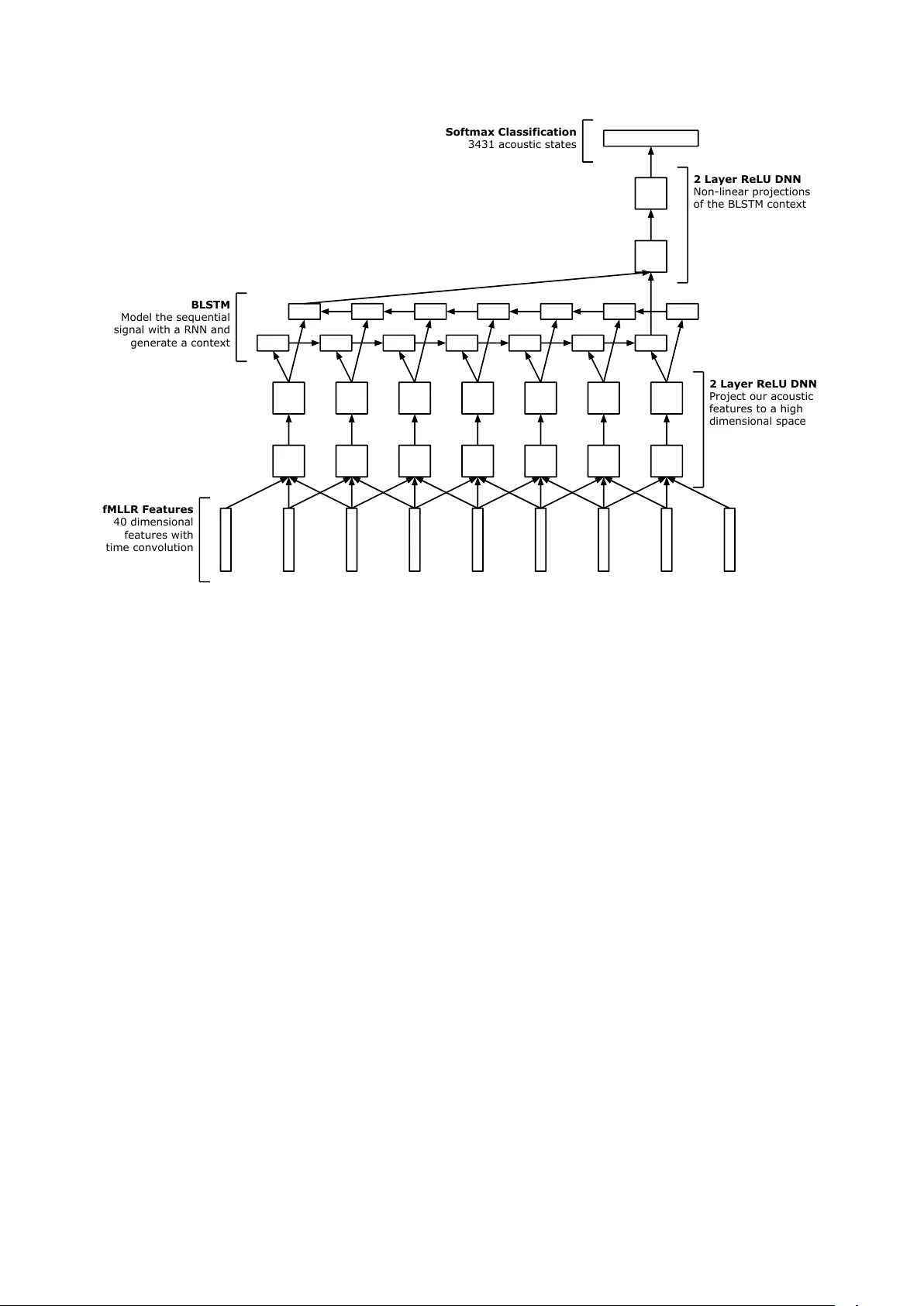
Deep Recurr ent Neural Networks f or Acoustic Modelling W illiam Chan 1 , Ian Lane 1 , 2 Carnegie Mellon Uni versity 1 Electrical and Computer Engineering, 2 Language T echnologies Institute williamchan@cmu.edu, lane@cmu.edu Abstract W e present a novel deep Recurrent Neural Network (RNN) model for acoustic modelling in Automatic Speech Recognition (ASR). W e term our contribution as a TC-DNN-BLSTM-DNN model, the model combines a Deep Neural Network (DNN) with T ime Con volution (TC), followed by a Bidirectional Long- Short T erm Memory (BLSTM), and a final DNN. The first DNN acts as a feature processor to our model, the BLSTM then gen- erates a conte xt from the sequence acoustic signal, and the final DNN takes the context and models the posterior probabilities of the acoustic states. W e achieve a 3.47 WER on the W all Street Journal (WSJ) ev al92 task or more than 8% relative impro ve- ment ov er the baseline DNN models Index T erms : Deep Neural Networks, Recurrent Neural Net- works, Long-Short T erm Memory , Asynchronous Stochastic Gradient Descent, Automatic Speech Recognition 1. Introduction Deep Neural Networks (DNNs) and Con v olutional Neural Net- works (CNNs) hav e yielded many state-of-the-art results in acoustic modelling for Automatic Speech Recognition (ASR) tasks [1, 2]. DNNs and CNNs often accept some spectral fea- ture (e.g., log-Mel filter banks) with a context windo w (e.g., +/- 10 frames) as inputs and trained via supervised backpropaga- tion with softmax targets learning the Hidden Markov Model (HMM) acoustic states. DNNs do not make much prior assumptions about the input feature space, and consequently the model architecture is blind to temporal and frequency structural localities. CNNs are able to directly model local structural localities through the usage of con v olutional filters. CNN filters connect to only a subset re- gion of the feature space and are tied and shared across the en- tire input feature, giving the model translational in variance [3]. Additionally , pooling is often added, which yields rotational in- variance [2]. The inherent structure of CNNs yields a model much more robust to small shifts and permutations. Speech is fundamentally a sequence of time signals. CNNs (with time con volution) can capture some of this time locality through the con volution filters, howe ver CNNs may not be able to directly capture longer temporal signal patterns. For exam- ple, temporal patterns may span 10 or more frames, howe v er the con v olution filter width may only be 5 frames wide. The CNN model must then rely on the higher le vel fully connected layers to model these long term dependencies. Additionally , one size may not fit all, the frame width of phones and temporal patterns are of v arying lengths. Optimizing the con v olution filter size is a expensi ve procedure and corpora dependent [4]. Recently , Recurrent Neural Networks (RNNs) have been introduced demonstrating po wer modelling capabilities for se- quences [5, 6, 7, 8]. RNNs incorporate feedback cycles in the network architecture. RNNs include a temporal memory com- ponent (for example, in LSTMs the cell state [9]), which allo ws the model to store temporal contextual information directly in the model. This relieves us from explicitly defining the size of temporal contexts (e.g., the time con v olution filter size in CNNs), and allows the model to learn this directly . In fact in [8], the whole speech sequence can be accumulated in the tem- poral context. There exist many implementations of RNNs [10]. LSTM and Gated Recurrent Units (GRUs) [10] are particular imple- mentations of RNNs that are easy to train and do not suffer from the vanishing or exploding gradient problems when perform- ing Backpropagation Through T ime (BPTT) [11]. LSTMs ha ve the capability to remember sequences with long range temporal dependencies [9] and have been applied successfully to many applications include image captioning [12], end-to-end speech recognition [13] and machine translation [14]. LSTMs process sequential signals in one direction. One natural extension is bidirectional LSTMs (BLSTMs), which is composed of two LSTMs. The forward LSTM process the se- quence as usual (e.g., reads the input sequence in the forward direction), the second processes the input sequence in backward order . The outputs of the two sequences can then be concate- nated. BLSTMs have two distinct advantages ov er LSTMs, the first advantage being the forward and backward passes of the se- quence yields differing temporal dependencies, the model can capture both sets of the signal dependencies. The second adv an- tage is the higher le vel sequence layers (e.g., stacked BLSTMs) using the BLSTM outputs can access information from both in- put directions. LSTMs and GRUs (and their bidirectional variants) ha ve re- cently been successfully applied to acoustic modelling and ASR [5, 7, 8]. In [5] TIMIT phone sequences were trained end-to- end from unse gmented sequence data using a LSTM transducer . LSTMs can be combined with Connectionist T emporal Classifi- cation (CTC) and implicitly perform sequence training o ver the speech signal on TIMIT [7]. [15] used GR Us and generated an explicit alignment model between the TIMIT speech sequence data to the phone sequence. In [8] a commercial speech sys- tem is trained using a LSTM acoustic model, here the the entire speech sequence is used as the context for classifying context dependent phones. [16] extend from [8] and applied sequence training on top of LSTMs. Our contrib ution in this paper is a novel deep RNN acoustic model which is easy to train and archiv es an 8% relati ve improvement over DNNs for the W all Street Journal (WSJ) corpus. 2. Model Our model architecture can be summarized as a TC-DNN- BLSTM-DNN acoustic model. Our model deals with fix ed fMLLR Features 40 dimensional features with time convolution 2 Layer ReLU DNN Project our acoustic features to a high dimensional space 2 Layer ReLU DNN Non-linear projections of the BLSTM context BLSTM Model the sequential signal with a RNN and generate a context Softmax Classification 3431 acoustic states Figure 1: TC-DNN-BLSTM-DNN Architecture. The model contains 3 parts, a signal processing DNN which takes in the original fMLLR acoustic features and projects them to a high dimensional space, a BLSTM which models the sequential signal and produces a context, and a final DNN which takes the conte xt generated by the BLSTM and estimates the likelihoods across acoustic states. length sequences (as opposed to variable length whole se- quences [8]) of a context window . The adv antage of our model is we can easily use BLSTMs online (e.g., we don’t need to wait to see the end of the sequence to generate the backward direction pass of the LSTM). The disadv antage is howe v er the amount of temporal information stored in the model is limited to the context width (e.g., similar to DNNs and CNNs). How- ev er , in offline decoding, we can also compute all the acoustic states in parallel (e.g., one big minibatch) versus the O ( T ) it- erations needed by [8] due to the iterative dependency of the LSTM memory . The model begins with a fixed window context of acous- tic features (e.g., fMLLR) similar to a standard DNN or CNN acoustic model [17, 3]. W ithin the context window , an over- lapping time window of features, or Time Con v olution (TC) of features is fed in at each timestep. A similar approach was used by [18], howev er they used a stride of 2 for the sake of reducing computational cost, howe ver , our motiv ation is time con v olution rather than performance and we use a stride of 1. The model processes these features with independent columns of DNNs ov er the context windo w timesteps. W e refer this as the TC-DNN component of the model. The objectiv e of the TC- DNN component is to project the original acoustic feature into a high dimensional feature space which can then be easily mod- elled or consumed by the LSTM. [19] refers to this as a Deep Input-to-Hidden Function. The transformed high dimensional acoustic signal is then fed into a BLSTM. The BLSTM models the time sequential component of the signal. Our LSTM implementation is similar to [12] and described in the equations below: i t = φ ( W xi x t + W hi h t − 1 ) (1) f t = φ ( W xf x t + W hf h t − 1 ) (2) c t = f t  cs t − 1 + i t  tanh( W xc x t + W hc h t − 1 ) (3) o t = φ ( W xo x t + W ho h t − 1 ) (4) h t = o t  tanh( c t ) (5) W e do not use bias, nor peephole connections; on initial experimentation, we observed negligible difference, hence we omitted them in this work. Additionally , we did not apply any gradient clipping or gradient projection, we did ho wev er apply a cell acti vation clipping of 3 to pre vent saturation in the sigmoid non-linearities. W e found the cell acti vation clipping to help re- mov e con vergence problems and exploding gradients. W e also do not use a recurrent projection layer [8]. W e found our LSTM implementation to train very easily without exploding gradients, ev en with high learning rates. The BLSTM scans our input acoustic window of time width T emitted by the first DNN and outputs two fixed va lue vector (one for each direction), which is then concatenated: c =  h f T h b 1  (6) W e refer c as the context of the acoustic signal generated by the BLSTM. Context c compresses the rele v ant acoustic infor- mation needed to classify the phones from the feature context (e.g., the window of fMLLR features). The context is further manipulated and projected by a sec- ond DNN. The second DNN adds additional non-linear trans- formations before being finally fed to the softmax layer to model the context dependent state posteriors. [19] refers this as the Deep Hidden-to-Output Function. The model is trained supervised with backpropagation minimizing the cross entropy loss. Figure 1 gives a visualization of our entire model. 3. Optimization W e found our LSTM models to be very easy to train and con- ver ge. W e initialize our LSTM layers with a uniform distri- bution U ( − 0 . 01 , 0 . 01) , and our DNN layers with a Gaussian distribution N (0 , 0 . 001) . W e clip our LSTM cell activ ations to 3, we did not need to apply any gradient clipping or gradient projection. W e train our model with Stochastic Gradient Descent (SGD) using a minibatch size of 128, we found using larger minibatches (e.g., 256) to give slightly worse WERs. W e used a simple geometric decay schedule, we start with a learning rate of 0.1 and multiply it by a factor of 0.5 ev ery epoch. W e hav e a learning rate floor of 0 . 00001 (e.g., the learning rate does not decay beyond this value). W e experimented with both classi- cal and Nesterov momentum, howe ver we found momentum to harm the final WER con v ergence slightly , hence we use no mo- mentum. W e apply the same optimization hyperparameters for all our experiments, it is possible using a slightly dif ferent de- cay schedule will yield better results. Our best model took 17 epochs to conv er ge or around 51 hours in wall clock time with a NVIDIA T esla K20 GPU. 4. Experiments and Results W e experiment with the WSJ dataset. W e use si284 with ap- proximately 81 hours of speech as the training set, de v93 as our dev elopment set and ev al92 as our test set. W e observe the WER of our de v elopment set after ev ery epoch, we stop training once the dev elopment set no longer improves. W e report the con- ver ged dev93 and the corresponding e val92 WERs. W e use the same fMLLR features generated from the Kaldi s5 recipe [20], and our decoding setup is e xactly the same as the s5 recipe (e.g., large dictionary and trigram pruned language model). W e use the tri4b GMM alignments as our training targets and there are a total of 3431 acoustic states. The GMM tri4b baseline achiev ed a dev and test WER of 9.39 and 5.39 respecti vely . 4.1. DNN T wo baseline DNN systems are presented, the first is the Kaldi s5 WSJ recipe with sigmoid DNN model which pretrains with a Deep Belief Network [21], it achie ved a WER of 3.81. W e also built a ReLU DNN which requires no pretraining. The ReLU DNN consisted of 4 layers of 2048 ReLU neurons followed by softmax and trained with geometrically decayed SGD. W e also experimented with deeper and wider networks, howe ver we found this 5 layer architecture to be the best. Our ReLU DNN is much easier to train (e.g., no e xpensi ve pretrain- ing) and achieves a WER of 3.79 matching the WER of the pre- trained Sigmoid DNN. The ReLU DNN results suggest that pre- training may not be necessary gi ven suf ficient supervised data and is competiti ve for the acoustic modelling task. T able 1 sum- marizes the WERs for our DNN baseline systems. T able 1: WERs for W all Str eet Journal. The ReLU DNN re- quir es no pretraining and matches the WER of the Kaldi s5 r ecipe which uses DBN pr etraining. Model dev93 WER ev al92 WER GMM Kaldi tri4b 9.39 5.39 DNN Kaldi s5 6.68 3.81 DNN ReLU 6.84 3.79 T able 2: BLSTM WERs for W all Str eet Journal. Larg er recur - r ent models tend to perform better without o verfitting. The deep BLSTM models do not yield any substantial gains over their single layer counterparts. Cell Size Layers dev93 WER eval92 WER 128 1 8.19 5.19 256 1 7.94 4.66 512 1 7.43 4.36 768 1 7.36 4.16 1024 1 7.23 4.06 256 2 7.54 4.36 512 2 7.40 4.25 4.2. Deep BLSTM W e experimented with single layer and two layer deep BLSTM models. The cell size reported is per direction (e.g., total cells are doubled). The BLSTM models take longer to train and underperform compared to the ReLU DNN model. The large BLSTM models tend to outperform the smaller ones, suggest- ing ov erfitting is not an issue. Ho wev er , there is limited incre- mental gain in WER performance with additional cells. Our best single layer BLSTM with 1024 bidirectional cells achiev ed only 4.06 WER compared to 3.79 from our ReLU DNN model. Deep BLSTM models [7] may giv e additional model per- formance, since the upper layers can access information from the shallow layers in both directions and additional layers of non-linearities are av ailable. Our deep BLSTM models contain two layers, the cell size reported is per direction per layer (e.g., total cells are quadrupled). Our deep BLSTM experiments gi ve mixed results. For the same number of cells per layer, the deep model performs slightly better . Ho wev er , if we fixed the number of parameters, the single layer BLSTM model performs slightly better , the single layer of 1024 bidirectional cells achieved a WER of 4 . 16 while the deep tw o layer BLSTM model with 512 bidirectional cells per layer achieved a WER 4 . 25 . T able 2 sum- marizes our BLSTM experiment WERs. 4.3. TC-DNN-BLSTM-DNN W e e xperimented next with a DNN-BLSTM model. Our DNN- BLSTM model does not have time con volution at its input, and lacks the second DNN non-linearities for conte xt projection. The two layer 2048 neuron ReLU DNN in front of the BLSTM acts as a signal processor , projecting the original acoustic signal (e.g., each fMLLR vector) into a new high dimensional space which can be more easily digested by the LSTM. The BLSTM module uses 128 bidirectional cells. Compared to the 128 bidi- rectional cell BLSTM model, the model improv es from 5.19 WER to 3.92 WER or 24% relati vely . The results of this e xper - iment suggest the fMLLR features may not be the best features for BLSTM models (to consume directly at least); b ut rather T able 3: Ablation effects of our TC-DNN-BLSTM-DNN model. The DNNs and T ime Convolution ar e used for signal and con- text pr ojections. W e show that all components are critical to obtain the best performing model. Model dev93 WER ev al92 WER DNN-BLSTM 7.40 3.92 BLSTM-DNN 6.90 3.84 DNN-BLSTM-DNN 7.19 3.76 TC-DNN-BLSTM-DNN 6.58 3.47 learnt features (through the DNN feature processor) can yield better features for the BLSTM model to consume. The next experiment we ran was a BLSTM-DNN model. Here, the BLSTM accepts the original acoustic feature without modification and emits a conte xt. The conte xt is passed through to a two layer 2048 neuron ReLU DNN which provides addi- tional layers of non-linear projections before classification by the softmax layer . Once again, the BLSTM module uses only 128 bidirectional cells. The model improv es from 5.19 WER to 3.84 WER or 26% relativ ely when compared to the original 128 bidirectional cell BLSTM model which does not hav e the con- text non-linearities. The result of this experiment suggest the LSTM context should not be used directly for softmax phone classification, but rather additional layers of non-linearities are needed to achiev e the best performance. W e then experimented with a DNN-BLSTM-DNN model (without time con volution). Each DNN has two layers of 2048 ReLU neurons, and the BLSTM layer had 128 cells per direc- tion. W e combine both the benefits of a learnt signal processing DNN and the context projection. Compared to a 128 bidirec- tional cell BLSTM model, our WER drops from 5.19 to 3.76 or 28% relatively . Compared to a 1024 bidirectional cell BLSTM model, we essentially redistributed our parameters from a wide shallow network to a deeper network. W e achiev e a 11% rela- tiv e impro vement compared to a single layer 1024 bidirectional cell BLSTM, suggesting the deeper models are much more ex- pressiv e and po werful. Finally , our TC-DNN-BLSTM-DNN model combines the DNN-BLSTM-DNN with input time con volution. Our model further improv es from 3.76 WER without time con volution to 3.47 WER with time conv olution. Compared to the DNN mod- els, we achie ve 0.32 absolute WER reduction or 8% relativ ely . T o the best of our knowledge, this is the best WSJ ev al92 per- formance without sequence training [22]. W e hypothesize the time con volution gives a richer signal representation to the DNN signal processor and consequently the BLSTM model to con- sume. The time con volution also relie ves the LSTM computa- tion power to learning long term dependencies, rather than short term dependencies. T able 3 summarizes the experiments for this section. 4.4. Distributed Optimization All results presented in the pre vious sections of this paper were trained with a single GPU with SGD. T o reduce the time re- quired to train an individual model we also e xperimented with distributed Asynchronous Stochastic Gradient Descent (ASGD) across multiple GPUs. Our implementation is similar to [23], we hav e 4 GPUs (NVIDIA T esla K20) in our system, 1 GPU is dedicated as a parameter server and we hav e 3 GPU compute shards (e.g., the independent SGD learners). W e do not apply T able 4: Effects of distributed optimization for our TC-DNN- BLSTM-DNN model. The ASGD experiments uses 3 indepen- dent SGD shar ds. Model Epochs Time (hrs) dev93 WER ev al92 WER SGD 17 51.5 6.58 3.47 ASGD 14 16.8 6.57 3.72 0 10 20 30 40 50 60 Time (Hours) 2 3 4 5 6 7 8 WER SGD dev93 SGD eval92 3x ASGD dev93 3x ASGD eval92 WER vs. TIme Figure 2: SGD vs x3 ASGD WER con ver gence comparison, each point represents one epoch of the respectiv e optimizer . any stale gradient decay [23] or warm starting [24]. W e use the exact same learning rate schedule, minibatch size and hyper- parameters as our TC-DNN-BLSTM-DNN SGD baseline. [8] applied distributed ASGD optimization, howe ver they applied it on a cluster of CPUs rather than GPUs. Additionally , [8] did not compare if there was a WER differential between SGD versus ASGD. Our baseline TC-DNN-BLSTM-DNN SGD system took 17 epochs or 51 wall clock hours to con ver ge to a dev and test WER of 6.58 and 3.47. Our distributed implementation conv erges in 14 epochs and 16.8 wall clock hours, achieves a dev and test WER of 6.57 and 3.72. The distributed optimization is able to match the dev WER, ho we ver the test WER is significantly worse. It is unclear whether this WER differential is due to the asynchronicity characteristic of the optimizer or due to the small datasets, we suspect with larger datasets the gap between the ASGD and SGD will shrink. The conclusion we draw is that ASGD can con ver ge much quicker and faster , howe ver there may be a impact to final WER performance. T able 4 and Figure 2 summarizes our results. 5. Conclusions In this paper , we presented a novel TC-DNN-BLSTM-DNN acoustic model architecture. On the WSJ eval92 task, we report a 3.47 WER or more than 8% relativ e improv ement over the DNN baseline of 3.79 WER. Our model is easy to optimize and implement, and does not suffer from exploding gradients e ven with high learning rates. W e also found that pretraining may not be necessary for DNNs, the DBN pretrained DNN achie ved a 3.81 WER compared to our ReLU DNN without pretraining of 3.79 WER. W e also experimented with ASGD with our TC- DNN-BLSTM-DNN model, we were able to match the SGD dev WER, howev er the WER on the evaluation set was signifi- cantly lo wer at 3.72. In future work, we seek to apply sequence training on top of our acoustic model to further improve the model accuracy . 6. References [1] N. Jaitly , P . Nguyen, A. W . Senior , and V . V anhoucke, “ Appli- cation of Pretrained Deep Neural Networks to Large V ocabulary Speech Recognition, ” in Interspeech , 2012. [2] T . Sainath, B. Kingsbury , A. rahman Mohamed, G. E. Dahl, G. Saon, H. Soltau, T . Beran, A. Y . Aravkin, and B. Ramabhad- ran, “Improvements to Deep Con v olutional Neural Networks for L VCSR, ” in Automatic Speech Recognition and Understanding W orkshop , 2013. [3] T . Sainath, A. rahman Mohamed, B. Kingsbury , and B. Ramab- hadran, “Deep Con volutional Neural Networks for L VCSR, ” in IEEE International Confer ence on Acoustics, Speech and Signal Pr ocessing , 2013. [4] W . Chan and I. Lane, “Deep Con v olutional Neural Networks for Acoustic Modeling in Low Resource Languages, ” in IEEE Inter- national Confer ence on Acoustics, Speech and Signal Pr ocessing , 2015. [5] A. Gra ves, “Sequence Transduction with Recurrent Neural Net- works, ” in International Confer ence on Machine Learning: Rep- r esentation Learning W orkshop , 2012. [6] A. Graves, A. rahman Mohamed, and G. Hinton, “Speech Recog- nition with Deep Recurrent Neural Networks, ” in IEEE Interna- tional Confer ence on Acoustics, Speech and Signal Pr ocessing , 2013. [7] A. Graves, N. Jaitly , and A. rahman Mohamed, “Hybrid Speech Recognition with Bidirectional LSTM, ” in Automatic Speech Recognition and Understanding W orkshop , 2013. [8] H. Sak, A. Senior , and F . Beaufays, “Long Short-T erm Memory Recurrent Neural Network Architectures for Large Scale Acoustic Modeling, ” in INTERSPEECH , 2014. [9] S. Hochreiter and J. Schmidhuber , “Long Short-T erm Memory , ” Neural Computation , vol. 9, no. 8, pp. 1735–1780, No vember 1997. [10] J. Chung, C. Gulcehre, K. Cho, and Y . Bengio, “Empirical Eval- uation of Gated Recurrent Neural Networks on Sequence Model- ing, ” in Neural Information Pr ocessing Systems: W orkshop Deep Learning and Repr esentation Learning W orkshop , 2014. [11] S. Hochreiter , Y . Bengio, P . Frasconi, and J. Schmidhuber, “Gradi- ent Flow in Recurrent Nets: the Difficulty of Learning Long-T erm Dependencies, ” 2011. [12] O. V inyals, A. T oshev , S. Bengio, and D. Erhan, “Show and T ell: A Neural Image Caption Generator, ” in , 2014. [13] A. Graves and N. Jaitly , “T owards End-to-End Speech Recogni- tion with Recurrent Neural Networks, ” in International Confer- ence on Machine Learning , 2014. [14] I. Sutskev er , O. V inyals, and Q. Le, “Sequence to Sequence Learn- ing with Neural Networks, ” in Neural Information Processing Systems , 2014. [15] J. Chorowski, D. Bahdanau, K. Cho, and Y . Bengio, “End-to-end Continuous Speech Recognition using Attention-based Recurrent NN: First Results, ” in Neural Information Processing Systems: W orkshop Deep Learning and Representation Learning W ork- shop , 2014. [16] H. Sak, O. V inyals, G. Heigold, A. Senior , E. McDermott, R. Monga, and M. Mao, “Sequence Discriminative Distributed T raining of Long Short-T erm Memory Recurrent Neural Net- works, ” in INTERSPEECH , 2014. [17] G. Hinton, L. Deng, D. Y u, G. Dahl, A. rahman Mohamed, N. Jaitly , A. Senior, V . V anhoucke, P . Nguyen, T . Sainath, and B. Kingsbury , “Deep Neural Networks for Acoustic Modeling in Speech Recognition, ” IEEE Signal Processing Magazine , Novem- ber 2012. [18] A. Hannun, C. Case, J. Casper, B. Catanzaro, G. Diamos, E. Elsen, R. Prenger , S. Satheesh, S. Sengupta, A. Coates, and A. Ng, “Deep Speech: Scaling up end-to-end speech recognition, ” in , 2014. [19] R. Pascanu, C. Gulcehre, K. Cho, and Y . Bengio, “How to Con- struct Deep Recurrent Neural Networks, ” in International Confer- ence on Learning Repr esentations , 2014. [20] D. Pov ey , A. Ghoshal, G. Boulianne, L. Burget, O. Glembek, N. Goel, M. Hannenmann, P . Motlicek, Y . Qian, P . Schwarz, J. Silovsk y , G. Stemmer, and K. V esely , “The Kaldi Speech Recognition T oolkit, ” in Automatic Speech Recognition and Un- derstanding W orkshop , 2011. [21] G. Hinton, S. Osindero, and Y .-W . T eh, “ A fast learning algorithm for deep belief nets, ” Neur al Computation , vol. 18, pp. 1527– 1554, July 2006. [22] K. V esely , A. Ghoshal, L. Bur get, and D. Pove y , “Sequence- discriminativ e training of deep neural networks, ” in INTER- SPEECH , 2013. [23] W . Chan and I. Lane, “Distributed Asynchronous Optimization of Con volutional Neural Netw orks, ” in INTERSPEECH , 2014. [24] J. Dean, G. S. Corrado, R. Monga, K. Chen, M. Devin, Q. V . Le, M. Z. Mao, M. Ranzato, A. Senior , P . T ucker , K. Y ang, and A. Y . Ng, “Large Scale Distributed Deep Networks, ” in Neural Information Pr ocessing Systems , 2012.