A Probabilistic Theory of Deep Learning

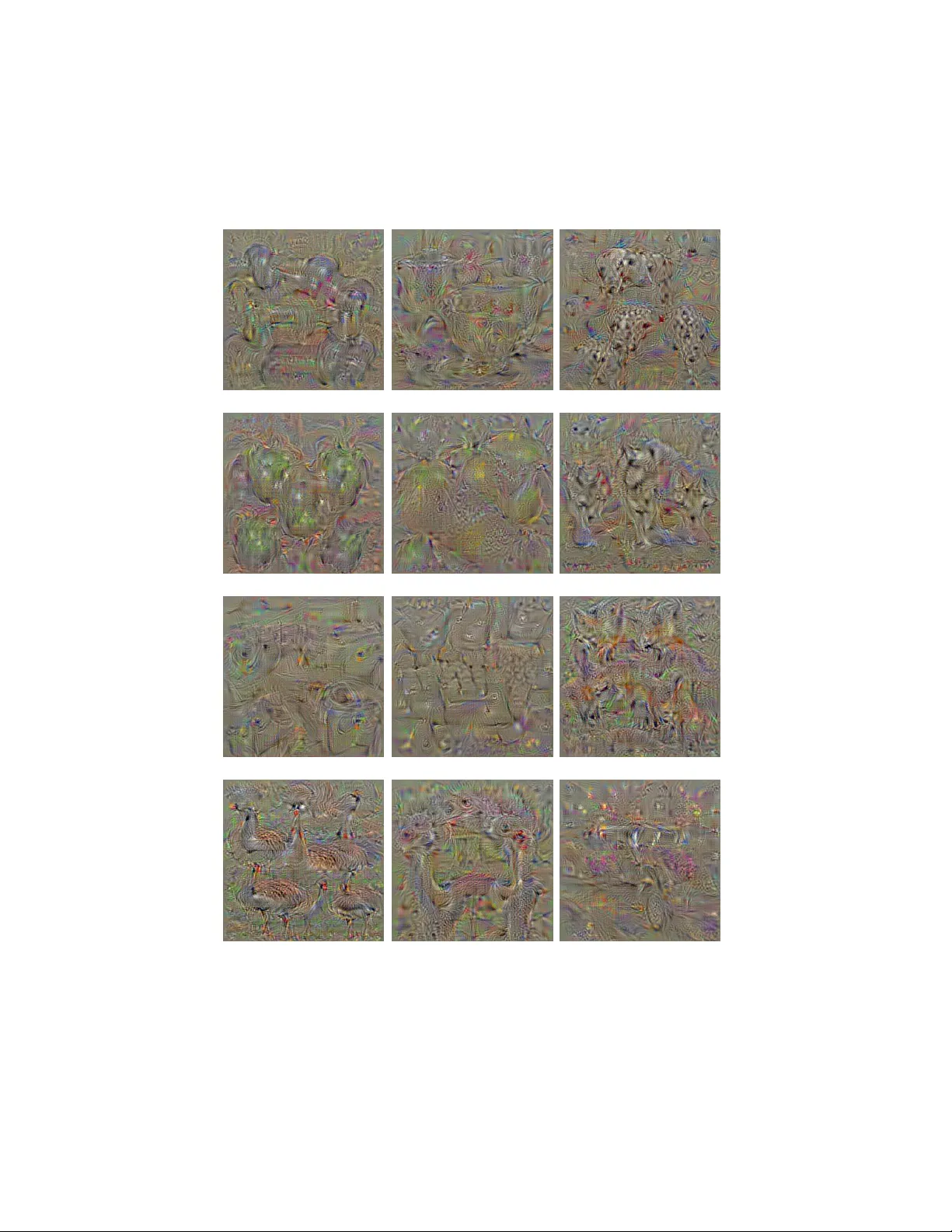
A Pr obabilistic Theory of Deep Lear ning Ankit B. Patel, T an Nguyen, Richard G. Baraniuk Department of Electrical and Computer Engineering Rice Uni versity { abp4, mn15, richb } @rice.edu April 2, 2015 A grand challenge in machine learning is the de velopment of computational al- gorithms that match or outperf orm humans in per ceptual inference tasks such as visual object and speech recognition. The key factor complicating such tasks is the presence of numer ous nuisance variables , f or instance, the unknown object position, orientation, and scale in object recognition or the unkno wn voice pronunciation, pitch, and speed in speech r ecognition. Recently , a new breed of deep learning algorithms ha ve emerged for high-nuisance infer ence tasks; they are constructed from many layers of alter nating linear and nonlin- ear processing units and ar e trained using large-scale algorithms and massiv e amounts of training data. The r ecent success of deep learning systems is im- pressi ve — they now r outinely yield pattern recognition systems with near- or super -human capabilities — b ut a fundamental question r emains: Why do they w ork? Intuitions abound, but a coherent framework for understanding, analyzing, and synthesizing deep learning ar chitectures has r emained elusive. W e answer this question by developing a new probabilistic framework f or deep learning based on a Bayesian generative probabilistic model that explicitly cap- tures variation due to nuisance variables. The graphical structure of the model enables it to be learned from data using classical expectation-maximization techniques. Furthermore, by relaxing the generati ve model to a discriminati ve one, we can reco ver two of the curr ent leading deep learning systems, deep con volutional neural netw orks (DCNs) and random decision f orests (RDFs), pro viding insights into their successes and shortcomings as well as a princi- pled route to their impr ovement. 1 Contents 1 Introduction 4 2 A Deep Probabilistic Model f or Nuisance V ariation 5 2.1 The Rendering Model: Capturing Nuisance V ariation . . . . . . . . . . . . . . 6 2.2 Deri ving the Ke y Elements of One Layer of a Deep Con volutional Network from the Rendering Model . . . . . . . . . . . . . . . . . . . . . . . 9 2.3 The Deep Rendering Model: Capturing Le vels of Abstraction . . . . . . . . . . 12 2.4 Inference in the Deep Rendering Model . . . . . . . . . . . . . . . . . . . . . 15 2.4.1 What About the SoftMax Regression Layer? . . . . . . . . . . . . . . 17 2.5 DCNs are Probabilistic Message Passing Netw orks . . . . . . . . . . . . . . . 17 2.5.1 Deep Rendering Model and Message Passing . . . . . . . . . . . . . . 17 2.5.2 A Unification of Neural Networks and Probabilistic Inference . . . . . 18 2.5.3 The Probabilistic Role of Max-Pooling . . . . . . . . . . . . . . . . . 18 2.6 Learning the Rendering Models . . . . . . . . . . . . . . . . . . . . . . . . . 18 2.6.1 EM Algorithm for the Shallow Rendering Model . . . . . . . . . . . . 20 2.6.2 EM Algorithm for the Deep Rendering Model . . . . . . . . . . . . . . 21 2.6.3 What About DropOut Training? . . . . . . . . . . . . . . . . . . . . . 23 2.7 From Generati ve to Discriminati ve Classifiers . . . . . . . . . . . . . . . . . . 23 2.7.1 Transforming a Generati ve Classifier into a Discriminati ve One . . . . 24 2.7.2 From the Deep Rendering Model to Deep Conv olutional Networks . . . 26 3 New Insights into Deep Con volutional Networks 27 3.1 DCNs Possess Full Probabilistic Semantics . . . . . . . . . . . . . . . . . . . 27 3.2 Class Appearance Models and Acti vity Maximization . . . . . . . . . . . . . . 27 3.3 (Dis)Entanglement: Supervised Learning of T ask T ar gets Is Intertwined with Unsupervised Learning of Latent T ask Nuisances . . . . . . . 30 4 From the Deep Rendering Model to Random Decision F orests 30 4.1 The Evolutionary Deep Rendering Model: A Hierarchy of Categories . . . . . 32 4.2 Inference with the E-DRM Y ields a Decision T ree . . . . . . . . . . . . . . . . 33 4.2.1 What About the Leaf Histograms? . . . . . . . . . . . . . . . . . . . . 34 4.3 Bootstrap Aggregation to Pre vent Overfitting Y ields A Decision Forest . . . . . . . . . . . . . . . . . . . . . . . . . . . . . . . . . . . . . . . 34 4.4 EM Learning for the E-DRM Y ields the InfoMax Principle . . . . . . . . . . . 36 2 5 Relation to Prior W ork 36 5.1 Relation to Mixture of Factor Analyzers . . . . . . . . . . . . . . . . . . . . . 36 5.2 i -Theory: In v ariant Representations Inspired by Sensory Cortex . . . . . . . . 37 5.3 Scattering T ransform: Achieving In v ariance via W av elets . . . . . . . . . . . . 38 5.4 Learning Deep Architectures via Sparsity . . . . . . . . . . . . . . . . . . . . 38 5.5 Google FaceNet: Learning Useful Representations with DCNs . . . . . . . . . 39 5.6 Renormalization Theory . . . . . . . . . . . . . . . . . . . . . . . . . . . . . 40 5.7 Summary of K ey Distinguishing Features of the DRM . . . . . . . . . . . . . 40 6 New Directions 41 6.1 More Realistic Rendering Models . . . . . . . . . . . . . . . . . . . . . . . . 41 6.2 Ne w Inference Algorithms . . . . . . . . . . . . . . . . . . . . . . . . . . . . 43 6.2.1 Soft Inference . . . . . . . . . . . . . . . . . . . . . . . . . . . . . . . 43 6.2.2 T op-Down Con volutional Nets: T op-Down Inference via the DRM . . . 43 6.3 Ne w Learning Algorithms . . . . . . . . . . . . . . . . . . . . . . . . . . . . 44 6.3.1 Deriv ati ve-Free Learning . . . . . . . . . . . . . . . . . . . . . . . . . 44 6.3.2 Dynamics: Learning from V ideo . . . . . . . . . . . . . . . . . . . . . 44 6.3.3 Training from Labeled and Unlabeled Data . . . . . . . . . . . . . . . 44 A Supplemental Information 46 A.1 From the Gaussian Rendering Model Classifier to Deep DCNs . . . . . . . . . 46 A.2 Generalizing to Arbitrary Mixtures of Exponential Family Distributions . . . . . . . . . . . . . . . . . . . . . . . . . . . . . . . . . . . 49 A.3 Regularization Schemes: Deriving the DropOut Algorithm . . . . . . . . . . . 49 3 1 Intr oduction Humans are expert at a wide array of complicated sensory inference tasks, from recognizing objects in an image to understanding phonemes in a speech signal, despite significant v ariations such as the position, orientation, and scale of objects and the pronunciation, pitch, and volume of speech. Indeed, the main challenge in many sensory perception tasks in vision, speech, and natural language processing is a high amount of such nuisance variation . Nuisance v ariations complicate perception, because they turn otherwise simple statistical inference problems with a small number of variables (e.g., class label) into much higher-dimensional problems. For ex- ample, images of a car tak en from dif ferent camera viewpoints lie on a highly curved, nonlinear manifold in high-dimensional space that is intertwined with the manifolds of myriad other ob- jects. The ke y challenge in dev eloping an inference algorithm is then how to factor out all of the nuisance variation in the input . Over the past fe w decades, a vast literature that approaches this problem from myriad different perspecti ves has de veloped, but the most difficult inference problems hav e remained out of reach. Recently , a ne w breed of machine learning algorithms hav e emerged for high-nuisance in- ference tasks, resulting in pattern recognition systems with sometimes super-human capabili- ties ( 1 ). These so-called deep learning systems share two common hallmarks. First, architec- turally , they are constructed from many layers of alternating linear and nonlinear processing units. Second, computationally , their parameters are learned using large-scale algorithms and massi ve amounts of training data. T wo examples of such architectures are the deep con volu- tional neural network (DCN), which has seen great success in tasks like visual object recogni- tion and localization ( 2 ), speech recognition ( 3 ), and part-of-speech recognition ( 4 ), and random decision for ests (RDFs) ( 5 ) for image segmentation. The success of deep learning systems is impressi ve, but a fundamental question remains: Why do the y work? Intuitions abound to ex- plain their success. Some explanations focus on properties of feature in variance and selecti vity de veloped o ver multiple layers, while others credit raw computational po wer and the amount of av ailable training data ( 1 ). Howe ver , beyond these intuitions, a coherent theoretical frame- work for understanding, analyzing, and synthesizing deep learning architectures has remained elusi ve. In this paper , we dev elop a new theoretical framework that provides insights into both the successes and shortcomings of deep learning systems, as well as a principled route to their de- sign and improvement. Our frame work is based on a gener ative pr obabilistic model that e xplic- itly captures variation due to latent nuisance variables . The Rendering Model (RM) e xplicitly models nuisance v ariation through a r endering function that combines the task-specific vari- ables of interest (e.g., object class in an object recognition task) and the collection of nuisance v ariables. The Deep Rendering Model (DRM) e xtends the RM in a hierarchical f ashion by ren- 4 dering via a product of affine nuisance transformations across multiple lev els of abstraction. The graphical structures of the RM and DRM enable inference via message passing, using, for e x- ample, the sum-product or max-sum algorithms, and training via the expectation-maximization (EM) algorithm. A key element of the frame work is the relaxation of the RM/DRM generati ve model to a discriminati ve one in order to optimize the bias-v ariance tradeof f. The DRM unites and subsumes two of the current leading deep learning based systems as max-sum messag e passing networks . That is, configuring the DRM with tw o dif ferent nuisance structures — Gaussian translational nuisance or ev olutionary additi ve nuisance — leads directly to DCNs and RDFs, respectiv ely . The intimate connection between the DRM and these deep learning systems provides a range of new insights into how and why they work, answering se veral open questions. Moreover , the DRM provides insights into how and why deep learning fails and suggests pathways to their impro vement. It is important to note that our theory and methods apply to a wide range of dif ferent in- ference tasks (including, for example, classification, estimation, regression, etc.) that feature a number of task-irrele vant nuisance variables (including, for example, object and speech recog- nition). Ho wev er , for concreteness of exposition, we will focus belo w on the classification problem underlying visual object recognition. This paper is org anized as follows. Section 2 introduces the RM and DRM and demonstrates step-by-step ho w they map onto DCNs. Section 3 then summarizes some of the ke y insights that the DRM provides into the operation and performance of DCNs. Section 4 proceeds in a similar fashion to deri ve RDFs from a v ariant of the DRM that models a hierarchy of categories. Section 6 closes the paper by suggesting a number of promising av enues for research, including se veral that should lead to improvement in deep learning system performance and generality . The proofs of se veral results appear in the Appendix. 2 A Deep Pr obabilistic Model f or Nuisance V ariation This section de velops the RM, a generati ve probabilistic model that e xplicitly captur es nuisance transformations as latent variables . W e show ho w inference in the RM corresponds to oper - ations in a single layer of a DCN. W e then extend the RM by defining the DRM, a rendering model with layers representing dif ferent scales or le vels of abstraction. Finally , we sho w that, after the application of a discriminativ e relaxation, inference and learning in the DRM corre- spond to feedforw ard propag ation and back propagation training in the DCN. This enables us to conclude that DCNs are probabilistic message passing networks, thus unifying the probabilistic and neural network perspecti ves. 5 2.1 The Rendering Model: Capturing Nuisance V ariation V isual object recognition is naturally formulated as a statistical classification problem. 1 W e are giv en a D -pixel, multi-channel image I of an object, with intensity I ( x, ω ) at pixel x and channel ω (e.g., ω = { red, green, blue } ). W e seek to infer the object’ s identity (class) c ∈ C , where C is a finite set of classes. 2 W e will use the terms “object” and “class” interchangeably . Gi ven a joint probabilistic model p ( I , c ) for images and objects, we can classify a particular image I using the maximum a posteriori (MAP) classifier ˆ c ( I ) = argmax c ∈C p ( c | I ) = argmax c ∈C p ( I | c ) p ( c ) , (1) where p ( I | c ) is the image likelihood, p ( c ) is the prior distribution ov er the classes, and p ( c | I ) ∝ p ( I | c ) p ( c ) by Bayes’ rule. Object recognition, like many other inference tasks, is complicated by a high amount of v ariation due to nuisance variables, which the abo ve formation ignores. W e adv ocate explicitly modeling nuisance v ariables by encapsulating all of them into a (possibly high-dimensional) parameter g ∈ G , where G is the set of all nuisances. In some cases, it is natural for g to be a transformation and for G to be endo wed with a (semi-)group structure. W e now propose a g enerative model for images that explicitly models the relationship be- tween images I of the same object c subject to nuisance g . First, gi ven c , g , and other auxiliary parameters, we define the r endering function R ( c, g ) that renders (produces) an image. In image inference problems, for e xample, R ( c, g ) might be a photorealistic computer graphics engine (c.f., Pixar). A particular realization of an image is then generated by adding noise to the output of the renderer: I | c, g = R ( c, g ) + noise . (2) W e assume that the noise distrib ution is from the e xponential f amily , which includes a large number of practically useful distrib utions (e.g., Gaussian, Poisson). Also we assume that the noise is independent and identically distributed (iid) as a function of pixel location x and that the class and nuisance v ariables are independently distrib uted according to cate gorical distri- butions. 3 W ith these assumptions, Eq. 2 then becomes the probabilistic (shallo w) Rendering 1 Recall that we focus on object recognition from images only for concreteness of exposition. 2 The restriction for C to be finite can be removed by using a nonparametric prior such as a Chinese Restaurant Process (CRP) ( 6 ) 3 Independence is merely a con venient approximation; in practice, g can depend on c . For example, humans hav e difficulty recognizing and discriminating upside do wn faces ( 7 ). 6 Model (RM) c ∼ Cat( { π c } c ∈C ) , g ∼ Cat( { π g } g ∈G ) , I | c, g ∼ Q ( θ cg ) . (3) Here Q ( θ cg ) denotes a distribution from the exponential family with parameters θ cg , which include the mixing probabilities π cg , natural parameters η ( θ cg ) , suf ficient statistics T ( I ) and whose mean is the rendered template µ cg = R ( c, g ) . An important special case is when Q ( θ cg ) is Gaussian, and this defines the Gaussian Ren- dering Model (GRM), in which images are generated according to I | c, g ∼ N ( I | µ cg = R ( c, g ) , Σ cg = σ 2 1 ) , (4) where 1 is the identity matrix. The GRM generalizes both the Gaussian Na ¨ ıve Bayes Classifier (GNBC) and the Gaussian Mixture Model (GMM) by allowing variation in the image to depend on an observ ed class label c , like a GNBC, and on an unobserved nuisance label g , like a GMM. The GNBC, GMM and the (G)RM can all be con veniently described as a directed gr aphical model ( 8 ). Figure 1A depicts the graphical models for the GNBC and GMM, while Fig. 1B sho ws how the y are combined to form the (G)RM. Finally , since the world is spatially varying and an image can contain a number of different objects, it is natural to break the image up into a number of (o verlapping) subimages, called patches , that are indexed by spatial location x . Thus, a patch is defined here as a collection of pixels centered on a single pix el x . In general, patches can ov erlap, meaning that (i) the y do not tile the image, and (ii) an image pixel x can belong to more than one patch. Gi ven this notion of pixels and patches, we allo w the class and nuisance v ariables to depend on pixel/patch location: i.e., local image class c ( x ) and local nuisance g ( x ) (see Fig. 2A). W e will omit the dependence on x when it is clear from context. The notion of a rendering operator is quite general and can refer to an y function that maps a target variable c and nuisance variables g into a pattern or template R ( c, g ) . For example, in speech recognition, c might be a phoneme, in which case g represents v olume, pitch, speed, and accent, and R ( c, g ) is the amplitude of the acoustic signal (or alternativ ely the time-frequency representation). In natural language processing, c might be the grammatical part-of-speech, in which case g represents syntax and grammar , and R ( c, g ) is a clause, phrase or sentence. T o perform object recognition with the RM via Eq. 1, we must mar ginalize out the nuisance v ariables g . W e consider two approaches for doing so, one con ventional and one uncon ven- tional. The Sum-Pr oduct RM Classifier (SP-RMC) sums o ver all nuisance variables g ∈ G and 7 I μ L μ L–1 μ 1 ... g L g L–1 g 1 A C B I c g I I c g Naive Bayes Classifier Mixture Model Rendering Model Deep Rendering Model Figure 1. Graphical depiction of the Nai ve Bayes Classifier (A, left), Gaussian Mixture Model (A, right), the shallow Rendering Model (B) and the Deep Rendering Model (C). All dependence on pixel location x has been suppressed for clarity . then chooses the most likely class: ˆ c SP ( I ) = argmax c ∈C 1 |G | X g ∈G p ( I | c, g ) p ( c ) p ( g ) = argmax c ∈C 1 |G | X g ∈G exp h η ( θ cg ) | T ( I ) i , (5) where h·|·i is the bra-k et notation for inner products and in the last line we hav e used the def- inition of an e xponential family distribution. Thus the SP-RM computes the marginal of the posterior distrib ution o ver the tar get v ariable, gi ven the input image. This is the con ventional approach used in most probabilistic modeling with latent v ariables. An alternati ve and less con ventional approach is to use the Max-Sum RM Classifier (MS- RMC), which maximizes ov er all g ∈ G and then chooses the most likely class: ˆ c MS ( I ) = argmax c ∈C max g ∈G p ( I | c, g ) p ( c ) p ( g ) = argmax c ∈C max g ∈G h η ( θ cg ) | T ( I ) i . (6) The MS-RMC computes the mode of the posterior distrib ution ov er the target and nuisance v ariables, giv en the input image. Equiv alently , it computes the most likely global configuration of tar get and nuisance variables for the image. Intuiti vely , this is an ef fectiv e strategy when there is one explanation g ∗ ∈ G that dominates all other explanations g 6 = g ∗ . This condition 8 is justified in settings where the rendering function is deterministic or nearly noise-free. This approach to classification is uncon ventional in both the machine learning and computational neuroscience literatures, where the sum-product approach is most commonly used, although it has recei ved some recent attention ( 9 ). Both the sum-product and max-sum classifiers amount to applying an af fine transformation to the input image I (via an inner product that performs feature detection via template match- ing), follo wed by a sum or max nonlinearity that marginalizes o ver the nuisance v ariables. Throughout the paper we will assume isotropic or diagonal Gaussian noise for simplicity , but the treatment presented here can be generalized to any distribution from the exponential family in a straightforw ard manner . Note that such an e xtension may require a non-linear trans- formation (i.e. quadratic or logarithmic T ( I ) ), depending on the specific exponential family . Please see Supplement Section A.2 for more details. 2.2 Deriving the K ey Elements of One Layer of a Deep Con volutional Network fr om the Rendering Model Having formulated the Rendering Model (RM), we now show ho w to connect the RM with deep con volutional networks (DCNs). W e will see that the MS-RMC (after imposing a fe w additional assumptions on the RM) gi ves rise to most commonly used DCN layer types. Our first assumption is that the noise added to the rendered template is isotropically Gaus- sian (GRM) i.e. each pixel has the same noise variance σ 2 that is independent of the config- uration ( c, g ) . Then, assuming the image is normalized k I k 2 = 1 , Eq. 6 yields the max-sum Gaussian RM classifier (see Appendix A.1 for a detailed proof) ˆ c MS ( I ) = argmax c ∈C max g ∈G  1 σ 2 µ cg    I  − 1 2 σ 2 k µ cg k 2 2 + ln π c π g ≡ argmax c ∈C max g ∈G h w cg | I i + b cg , (7) where we ha ve defined the natural parameter s η ≡ { w cg , b cg } in terms of the traditional pa- rameter s θ ≡ { σ 2 , µ cg , π c , π g } according to 4 w cg ≡ 1 σ 2 µ cg = 1 σ 2 R ( c, g ) b cg ≡ 1 2 σ 2 k µ cg k 2 2 + ln π c π g . (8) Note that we hav e suppressed the parameters’ dependence on pixel location x . 4 Since the Gaussian distribution of the noise is in the exponential family , it can be reparametrized in terms of the natural parameters. This is known as canonical form . 9 W e will no w demonstrate that the sequence of operations in the MS-RMC in Eq. 7 coincides exactly with the operations in volv ed in one layer of a DCN (or , more generally , a max-out neural network ( 10 )): image normalization, linear template matching, thresholding, and max pooling. See Fig. 2C. W e no w explore each operation in Eq. 7 in detail to make the link precise. First, the image is normalized . Until recently , there were se veral different types of normal- ization typically employed in DCNs: local response normalization, and local contrast normal- ization ( 11, 12 ). Ho wever , the most recent highly performing DCNs emplo y a different form of normalization, known as batch-normalization ( 13 ). W e will come back to this later when we sho w how to deri ve batch normalization from a principled approach. One implication of this is that it is unclear what probabilistic assumption the older forms of normalization arise from, if any . Second, the image is filtered with a set of noise-scaled rendered templates w cg . The size of the templates depends on the size of the objects of class c and the v alues of the nuisance v ariables g . Large objects will ha ve large templates, corresponding to a fully connected layer in a DCN ( 14 ), while small objects will hav e small templates, corresponding to a locally connected layer in a DCN ( 15 ). If the distribution of objects depends on the pix el position x (e.g., cars are more lik ely on the ground while planes are more lik ely in the air) then, in general, we will need dif ferent rendered templates at each x . In this case, the locally connected layer is appropriate. If, on the other hand, all objects are equally likely to be present at all locations throughout the entire image, then we can assume translational in variance in the RM. This yields a global set of templates that are used at all pixels x , corresponding to a con volutional layer in a DCN ( 14 ) (see Appendix A.2 for a detailed proof). If the filter sizes are lar ge relativ e to the scale at which the image variation occurs and the filters are overcomplete, then adjacent filters ov erlap and waste computation. In these case, it is appropriate to use a strided con volution, where the output of the traditional con volution is do wn-sampled by some factor; this sav es some computation without losing information. Third, the resulting activ ations (log-probabilities of the hypotheses) are passed through a pooling layer; i.e., if g is a translational nuisance, then taking the maximum ov er g corresponds to max pooling in a DCN. Fourth, recall that a giv en image pixel x will reside in se veral o verlapping image patches, each rendered by its o wn parent class c ( x ) and the nuisance location g ( x ) (Fig. 2A). Thus we must consider the possibility of collisions : i.e. when two different parents c ( x 1 ) 6 = c ( x 2 ) might render the same pixel (or patch). T o av oid such undesirable collisions, it is natural to force the rendering to be locally sparse : i.e. we must enforce that only one renderer in a local neighborhood can be “acti ve”. T o formalize this, we endo w each parent renderer with an ON/OFF state via a switching v ariable a ∈ A ≡ { ON , OFF } . If a = ON = 1 , then the rendered image patch is left untouched, 10 1" 2" 3" 4" g l +1 ON OF F a l +1 1 " 2" 4 " 3" x l c l x l +1 c l +1 µ  c l +1  µ  c l  = ⇤ l +1  g l +1  µ  c l +1  noise . . . 1" 2" 4" 3" x l c l x l +1 c l +1 . . . DC N C on volu tio n Ma x Po o l + RE LU In p u t Fe a t u r e Ma p Out pu t Fe a t u r e Ma p I l +1 Inference Discriminative Counterpart Probabilistic Model (Deep Rendering Model) A Factor Graph (Inference via Max-Sum) B Neural Network (Deep Convolutional Network) C 1" 2" 4" 3" x l c l x l +1 c l +1 max g l +1 {·} µ  c l +1  | µ  c l  ,g l +1 . . . Ma x  Sum Me s s a g e Ma x  Sum Me s s a g e Fa c t o r I l +1 h W l +1 |· i 1" 2" 3" 4" g l +1 ON OF F a l +1 I l I l Rendering In f e r e n c e In f e r e n c e . . . . . . . . . I 0 I 0 I 0 Figure 2. An e xample of mapping from the Deep Rendering Model (DRM) to its corresponding factor graph to a Deep Con volutional Network (DCN) showing only the transformation from lev el ` of the hierarchy of abstraction to lev el ` + 1 . (A) DRM generati ve model: a single super pix el x ` +1 at lev el ` + 1 (green, upper) renders do wn to a 3 × 3 image patch at lev el ` (green, lower), whose location is specified by g ` +1 (red). (B) Factor graph representation of the DRM model that supports efficient inference algorithms such as the max-sum message passing sho wn here. (C) Computational network that implements the max-sum message passing algorithm from (B) explicitly ; its structure exactly matches that of a DCN. 11 whereas if a = OFF = 0 , the image patch is masked with zeros after rendering. Thus, the switching v ariable a models (in)activ e parent renderers. Ho wev er , these switching v ariables hav e strong correlations due to the cro wding out effect: if one is ON, then its neighbors must be OFF in order to prev ent rendering collisions. Although natural for realistic rendering, this complicates inference. Thus, we employ an approxima- tion by instead assuming that the state of each renderer ON or OFF completely at random and thus independent of any other variables, including the measurements (i.e., the image itself). Of course, an approximation to real rendering, but it simplifies inference, and leads directly to rectified linear units, as we show below . Such approximations to true sparsity hav e been extensi vely studied, and are kno wn as spike-and-slab sparse coding models (16, 17) . Since the switching v ariables are latent (unobserved), we must max-marginalize over them during classification, as we did with nuisance variables g in the last section (one can think of a as just another nuisance). This leads to (see Appendix A.3 for a more detailed proof) ˆ c ( I ) = argmax c ∈C max g ∈G max a ∈A  1 σ 2 aµ cg    I  − 1 2 σ 2 ( k aµ cg k 2 2 + k I k 2 2 )) + ln π c π g π a ≡ argmax c ∈C max g ∈G max a ∈A a ( h w cg | I i + b cg ) + b cg a = argmax c ∈C max g ∈G ReLU ( h w cg | I i + b cg ) , (9) where b cg a and b cg are bias terms and ReLu ( u ) ≡ ( u ) + = max { u, 0 } denotes the soft-thresholding operation performed by the Rectified Linear Units (ReLU) in modern DCNs ( 18 ). In the last line, we have assumed that the prior π cg is uniform so that b cg a is independent of c and g and can be dropped. 2.3 The Deep Rendering Model: Capturing Lev els of Abstraction The world is summarizable at varying le vels of abstraction, and Hierarchical Bayesian Models (HBMs) can exploit this fact to accelerate learning. In particular , the power of abstraction allows the higher le vels of an HBM to learn concepts and categories far more rapidly than lo wer le vels, due to stronger inductiv e biases and exposure to more data ( 19 ). This is informally known as the Blessing of Abstraction ( 19 ). In light of these benefits, it is natural for us to e xtend the RM into an HBM, thus gi ving it the power to summarize data at dif ferent lev els of abstraction. In order to illustrate this concept, consider the example of rendering an image of a face, at dif ferent lev els of detail ` ∈ { L, L − 1 , . . . , 0 } . At level ` = L (the coarsest lev el of abstraction), we specify only the identity of the face c L and its ov erall location and pose g L without specifying any finer -scale details such as the locations of the eyes or type of facial expression. At lev el ` = L − 1 , we specify finer-grained details, such as the existence of a left e ye ( c L − 1 ) with a 12 Figure 3. This sculpture by Henri Matisse illustrates the Deep Rendering Model (DRM). The sculpture in the leftmost panel is analogous to a fully rendered image at the lowest abstraction le vel ` = 0 . Moving from left to right, the sculptures become progressiv ely more abstract, until the in the rightmost panel we reach the highest abstraction level ` = 3 . The finer -scale details in the first three panels that are lost in the fourth are the nuisance parameters g , whereas the coarser -scale details in the last panel that are preserved are the tar get c . certain location, pose, and state (e.g., g L − 1 = open or closed), again without specifying any finer-scale parameters (such as eyelash length or pupil shape). W e continue in this way , at each le vel ` adding finer -scaled information that was unspecified at lev el ` − 1 , until at lev el ` = 0 we ha ve fully specified the image’ s pixel intensities, leaving us with the fully rendered, multi-channel image I 0 ( x ` , ω ` ) . Here x ` refers to a pixel location at le vel ` . For another illustrati ve example, consider The Bac k Series of sculptures by the artist Henri Matisse (Fig. 3). As one moves from left to right, the sculptures become increasingly abstract, losing lo w-lev el features and details, while preserving high-le vel features essential for the o ver - all meaning: i.e. ( c L , g L ) = “woman with her back facing us. ” Con versely , as one mo ves from right to left, the sculptures become increasingly concrete, progressi vely gaining finer -scale de- tails (nuisance parameters g ` , ` = L − 1 , . . . , 0 ) and culminating in a rich and textured rendering. W e formalize this process of progressi ve rendering by defining the Deep Rendering Model (DRM). Analogous to the Matisse sculptures, the image generation process in a DRM starts at the highest lev el of abstraction ( ` = L ), with the random choice of the object class c L and overall pose g L . It is then follo wed by generation of the lower -le vel details g ` , and a progressiv e lev el- by-le vel ( ` → ` − 1 ) rendering of a set of intermediate rendered “images” µ ` , each with more detailed information. The process finally culminates in a fully rendered D 0 ≡ D -dimensional 13 image µ 0 = I 0 ≡ I ( ` = 0 ). Mathematically , c L ∼ Cat( π ( c L )) , c L ∈ C L , g ` +1 ∼ Cat( π ( g ` +1 )) , g ` +1 ∈ G ` +1 , ` = L − 1 , L − 2 , . . . , 0 µ ( c L , g ) = Λ( g ) µ ( c L ) ≡ Λ 1 ( g 1 ) · · · Λ L ( g L ) · µ ( c L ) , g = { g ` } L ` =1 I ( c L , g ) = µ ( c L , g ) + N (0 , σ 2 1 D ) ∈ R D . (10) Here C ` , G ` are the sets of all tar get-relev ant and tar get-irrelev ant nuisance v ariables at le vel ` , respecti vely . The r endering path is defined as the sequence ( c L , g L , . . . , g ` , . . . , g 1 ) from the root (o verall class) down to the individual pixels at ` = 0 . µ ( c L ) is an abstract template for the high-le vel class c L , and Λ( g ) ≡ Q ` Λ ` ( g ` ) represents the sequence of local nuisance transformations that renders finer -scale details as one mov es from abstract to concrete. Note that each Λ ` ( g ` ) is an affine transformation with a bias term α ( g ` ) that we hav e suppressed for clarity 5 . Figure 2A illustrates the corresponding graphical model. As before, we hav e suppressed the dependence of c ` , g ` on the pixel location x ` at le vel ` of the hierarchy . W e can cast the DRM into an incremental form by defining an intermediate class c ` ≡ ( c L , g L , . . . , g ` +1 ) that intuitiv ely represents a partial rendering path up to le vel ` . Then, the partial rendering from le vel ` + 1 to ` can be written as an af fine transformation µ ( c ` ) = Λ ` +1 ( g ` +1 ) · µ ( c ` +1 ) + α ( g ` +1 ) + N (0 , Ψ ` +1 ) , (11) where we have sho wn the bias term α explicitly and introduced noise 6 with a diagonal co- v ariance Ψ ` +1 . It is important to note that c ` , g ` can correspond to different kinds of target rele vant and irrele vant features at dif ferent le vels. For e xample, when rendering faces, c 1 ( x 1 ) might correspond to dif ferent edge orientations and g 1 ( x 1 ) to different edge locations in patch x 1 , whereas c 2 ( x 2 ) might correspond to dif ferent eye types and g 2 ( x 2 ) to dif ferent eye gaze directions in patch x 2 . The DRM generates images at intermediate abstraction le vels via the incr emental r endering functions in Eq. 11 (see Fig. 2A). Hence the complete rendering function R ( c, g ) from Eq. 2 is a composition of incremental rendering functions, amounting to a product of affine trans- formations as in Eq. 10. Compared to the shallo w RM, the factorized structure of the DRM results in an e xponential r eduction in the number of fr ee parameters , from D 0 |C L | Q ` |G ` | to |C L | P ` D ` |G ` | where D ` is the number of pix els in the intermediate image µ ` , thus enabling more ef ficient inference and learning, and most importantly , better generalization. 5 This assumes that we are using an exponential family with linear sufficient statistics i.e. T ( I ) = ( I , 1) T . Howe ver , note that the family we use here is not Gaussian, it is instead a Factor Analyzer , a different probabilistic model. 6 W e introduce noise for two reasons: (1) it will make it easier to connect later to existing EM algorithms for factor analyzers and (2) we can always take the noise-free limit to impose cluster well-separatedness if needed. Indeed, if the rendering process is deterministic or nearly noise-free, then the latter is justified. 14 The DRM as formulated here is distinct from but related to sev eral other hierarchical models, such as the Deep Mixture of F actor Analyzers (DMF A) ( 20 ) and the Deep Gaussian Mixture Model ( 21 ), both of which are essentially compositions of another model — the Mixture of Factor Analyzers (MF A) ( 22 ). W e will highlight the similarities and dif ferences with these models in more detail in Section 5. 2.4 Inference in the Deep Rendering Model Inference in the DRM is similar to inference in the shallo w RM. For example, to classify images we can use either the sum-product (Eq. 5) or the max-sum (Eq. 6) classifier . The ke y dif ference between the deep and shallow RMs is that the DRM yields iterated layer-by-layer updates, from fine-to-coarse abstraction (bottom-up) and from coarse-to-fine abstraction (top-down). In the case we are only interested in inferring the high-lev el class c L , we only need the fine-to-coarse pass and so we will only consider it in this section. Importantly , the bottom-up pass leads directly to DCNs, implying that DCNs ignore poten- tially useful top-down information. This maybe an explanation for their dif ficulties in vision tasks with occlusion and clutter , where such top-do wn information is essential for disambiguat- ing local bottom-up hypotheses. Later on in Section 6.2.2, we will describe the coarse-to-fine pass and a ne w class of T op-Down DCNs that do make use of such information. Gi ven an input image I 0 , the max-sum classifier infers the most likely global configuration { c ` , g ` } , ` = 0 , 1 , . . . , L by executing the max-sum message passing algorithm in two stages: (i) from fine-to-coarse lev els of abstraction to infer the ov erall class label ˆ c L MS and (ii) from coarse- to-fine le vels of abstraction to infer the latent v ariables ˆ c ` MS and ˆ g ` MS at all intermediate le vels ` . As mentioned above , we will focus on the fine-to-coarse pass. Since the DRM is an RM with a hierarchical prior on the rendered templates, we can use Eq. 7 to deriv e the fine-to-coarse 15 max-sum DRM classifier (MS-DRMC) as: ˆ c M S ( I ) = argmax c L ∈C max g ∈G h η ( c L , g ) | Σ − 1 | I 0 i = argmax c L ∈C max g ∈G h Λ( g ) µ ( c L ) | (Λ( g )Λ( g ) T ) † | I 0 i = argmax c L ∈C max g ∈G h µ ( c L ) | 1 Y ` = L Λ ` ( g ` ) † | I 0 i = argmax c L ∈C h µ ( c L ) | 1 Y ` = L max g ` ∈G ` Λ ` ( g ` ) † | I 0 i = argmax c L ∈C h µ ( c L ) | max g L ∈G L Λ L ( g L ) † · · · max g 1 ∈G 1 Λ 1 ( g 1 ) † | I 0 | {z } ≡ I 1 i ≡ argmax c L ∈C h µ ( c L ) | max g L ∈G L Λ L ( g L ) † · · · max g 2 ∈G 2 Λ 2 ( g 2 ) † | I 1 | {z } ≡ I 2 i ≡ argmax c L ∈C h µ ( c L ) | max g L ∈G L Λ L ( g L ) † · · · max g 3 ∈G 3 Λ 3 ( g 3 ) † | I 2 i . . . ≡ argmax c L ∈C h µ ( c L ) | I L i , (12) where Σ ≡ Λ( g )Λ( g ) T is the cov ariance of the rendered image I and h x | M | y i ≡ x T M y . Note the significant change with respect to the shallow RM: the cov ariance Σ is no longer diagonal due to the iterativ e affine transformations during rendering (Eq. 11), and so we must decorrelate the input image (via Σ − 1 I 0 in the first line) in order to classify accurately . Note also that we ha ve omitted the bias terms for clarity and that M † is the pseudoin verse of matrix M . In the fourth line, we used the distributi vity of max over products 7 and in the last lines defined the intermediate quantities I ` +1 ≡ max g ` +1 ∈G ` +1 h (Λ ` +1 ( g ` +1 )) † | {z } ≡ W ` +1 | I ` i = max g ` +1 ∈G ` +1 h W ` +1 ( g ` +1 ) | I ` i ≡ MaxP o ol(Con v ( I ` )) . (13) Here I ` = I ` ( x ` , c ` ) is the featur e map output of layer ` indexed by channels c ` and η ( c ` , g ` ) ∝ µ ( c ` , g ` ) are the natural parameters (i.e., intermediate rendered templates) for le vel ` . 7 For a > 0 , max { ab, ac } = a max { b, c } . 16 If we care only about inferring the ov erall class of the image c L ( I 0 ) , then the fine-to-coarse pass suf fices, since all information relev ant to determining the o verall class has been integrated. That is, for high-lev el classification, we need only iterate Eqs. 12 and 13. Note that Eq. 12 simplifies to Eq. 9 when we assume sparse patch rendering as in Section 2.2. Coming back to DCNs, we ha ve see that the ` -th iteration of Eq. 12 or Eq. 9 corresponds to feedforward propagation in the ` -th layer of a DCN. Thus a DCN’ s operation has a pr obabilistic interpr etation as fine-to-coarse infer ence of the most pr obable global configuration in the DRM. 2.4.1 What About the SoftMax Regression Lay er? It is important to note that we ha ve not fully reconstituted the architecture of modern a DCN as yet. In particular , the SoftMax regression layer , typically attached to the end of network, is missing. This means that the high-le vel class c L in the DRM (Eq. 12) is not necessarily the same as the training data class labels ˜ c giv en in the dataset. In fact, the two labels ˜ c and c L are in general distinct. But then how are we to interpr et c L ? The answer is that the most probable global con- figuration ( c L , g ∗ ) inferred by a DCN can be interpreted as a good r epr esentation of the input image, i.e., one that disentangles the many nuisance factors into (nearly) independent compo- nents c L , g ∗ . 8 Under this interpretation, it becomes clear that the high-lev el class c L in the disentangled representation need not be the same as the training data class label ˜ c . The disentangled representation for c L lies in the penultimate layer acti v ations: ˆ a L ( I n ) = ln p ( c L , g ∗ | I n ) . Gi ven this representation, we can infer the class label ˜ c by using a simple linear classifier such as the SoftMax re gression 9 . Explicitly , the Softmax regression layer computes p (˜ c | ˆ a L ; θ Softmax ) = φ ( W L +1 ˆ a L + b L +1 ) , and then chooses the most lik ely class. Here φ ( · ) is the softmax function and θ Softmax ≡ { W L +1 , b L +1 } are the parameters of the SoftMax re gression layer . 2.5 DCNs are Pr obabilistic Message Passing Networks 2.5.1 Deep Rendering Model and Message Passing Encouraged by the correspondence identified in Section 2.4, we step back for a moment to reinterpret all of the major elements of DCNs in a probabilistic light. Our deriv ation of the DRM inference algorithm abov e is mathematically equi v alent to performing max-sum message passing on the factor gr aph r epresentation of the DRM , which is shown in Fig. 2B. The factor 8 In this sense, the DRM can be seen as a deep (nonlinear) generalization of Independent Components Analysis ( 23 ). 9 Note that this implicitly assumes that a good disentangled representation of an image will be useful for the classification task at hand. 17 graph encodes the same information as the generati ve model but organizes it in a manner that simplifies the definition and ex ecution of inference algorithms ( 24 ). Such inference algorithms are called message passing algorithms, because they work by passing real-valued functions called messages along the edges between nodes. In the DRM/DCN, the messages sent from finer to coarser lev els are the feature maps I ` ( x ` , c ` ) . Howe ver , unlike the input image I 0 , the channels c ` in these feature maps do not refer to colors (e.g, red, green, blue) b ut instead to more abstract features (e.g., edge orientations or the open/closed state of an eyelid). 2.5.2 A Unification of Neural Networks and Pr obabilistic Inference The factor graph formulation provides a powerful interpretation that the con volution, Max- P ooling and ReLu operations in a DCN corr espond to max-sum infer ence in a DRM . Thus, we see that architectures and layer types commonly used in today’ s DCNs are not ad hoc; rather they can be deri ved from precise probabilistic assumptions that entirely determine their struc- ture. Thus the DRM unifies two perspectiv es — neural network and probabilistic inference. A summary of the relationship between the two perspecti ves is giv en in T able 1. 2.5.3 The Probabilistic Role of Max-P ooling Consider the role of max-pooling from the message passing perspecti ve. W e see that it can be interpreted as the “max” in max-sum, thus e xecuting a max-marginalization over nuisance v ariables g . T ypically , this operation would be intractable, since there are exponentially many configurations g ∈ G . But here the DRM’ s model of abstraction — a deep product of af fine transformations — comes to the rescue. It enables us to con vert an otherwise intractable max-marginalization ov er g into a tractable sequence of iterated max-marginalizations over abstraction le vels g ` (Eqs. 12, 13). 10 Thus, the max-pooling oper ation implements pr obabilistic mar ginalization, so is absolutely essential to the DCN’s ability to factor out nuisance variation. Indeed, since the ReLu can also be cast as a max-pooling over ON/OFF switching v ariables, we conclude that the most important operation in DCNs is max-pooling . This is in conflict with some recent claims to the contrary ( 27 ). 2.6 Learning the Rendering Models Since the RM and DRM are graphical models with latent v ariables, we can learn their pa- rameters from training data using the expectation-maximization (EM) algorithm ( 28 ). W e first de velop the EM algorithm for the shallow RM from Section 2.1 and then e xtend it to the DRM from Section 2.3. 10 This can be seen, equiv alently , as the execution of the max-product algorithm ( 26 ). 18 Aspect ! Neura l'Net s'P erspect iv e' ! Deep$ Convnet s$(DCNs ) ! Probabili stic+P erspectiv e+ ! Deep$ Render ing$Mod el$( DRM) ! Model ! Weigh ts and biases of f ilter s at a given layer Partial Rendering at a given abstraction le vel/scale ! Number of Layers Number of Abstraction Levels ! Number of Filters in a layer Number of Clusters /Classes at a given abstraction level ! Implicit in netw ork weights; can be computed by product of weights over all layers o r by activity maximizat ion Category pr ototypes are finel y detailed versions of coarser - scal e super - category prototypes. Fine details are modeled with affine nuisance transfor mations. Inference ! Forward propagat ion thru D CN Exact bottom - up inferen ce via Max - Sum Mess age Pas sing (wit h Ma x - Product for Nu isance Factorization). ! Input and Output Fe ature Maps Probabilistic Max - Sum Mess age s (real - valued functio ns of variables nodes) ! Template matching at a given layer (convolutional, locally or fully connected) Local computation at fac tor node (log - likelihood of mea surements) ! Max - Pooling over l ocal pooling region Max - Margi naliza tion o ver L atent Translational Nu isance transform a tions ! Rectifie d Linear Unit (ReL U). Spar sifi es ou tput activ ation s. Max - Margi naliza tion o ver L atent Swit chin g sta te of Rend erer. Low prior probabilit y of being ON. Learning ! Stoc hast ic Gra dien t Des cent Batch Disc riminative EM Algorithm with Fi ne - to - Coarse E - ste p + Gr adient M - step . No coarse - to - fine pass in E - step. ! N/A Full EM Alg orithm ! Batch - Normalized S GD (Google state - of - the - art [ BN ] ) Discrim inative Appro ximation to Full EM (assumes Diagonal Pixel Covariance ) ! T able 1. Summary of probabilistic and neural network perspectives for DCNs. The DRM provides an exact correspondence between the two, providing a probabilistic interpretation for all of the common elements of DCNs relating to the underlying model, inference algorithm, and learning rules. [BN] = reference ( 25 ). 19 2.6.1 EM Algorithm f or the Shallow Rendering Model Gi ven a dataset of labeled training images { I n , c n } N n =1 , each iteration of the EM algorithm con- sists of an E-step that infers the latent v ariables gi ven the observed v ariables and the “old” pa- rameters ˆ θ old gen from the last M-step, follo wed by an M-step that updates the parameter estimates according to E-step: γ ncg = p ( c, g | I n ; ˆ θ old gen ) , (14) M-step: ˆ θ = argmax θ X n X cg γ ncg L ( θ ) . (15) Here γ ncg are the posterior probabilities over the latent mixture components (also called the r esponsibilities ), the sum P cg is over all possible global configurations ( c, g ) ∈ C × G , and L ( θ ) is the complete-data log-likelihood for the model. For the RM, the parameters are defined as θ ≡ { π c , π g , µ cg , σ 2 } and include the prior prob- abilities of the different classes π c and nuisance variables π g along with the rendered templates µ cg and the pixel noise v ariance σ 2 . If, instead of an isotropic Gaussian RM, we use a full- cov ariance Gaussian RM or an RM with a different exponential family distribution, then the suf ficient statistics and the rendered template parameters would be different (e.g. quadratic for a full cov ariance Gaussian). When the clusters in the RM are well-separated (or equiv alently , when the rendering intro- duces little noise), each input image can be assigned to its nearest cluster in a “hard” E-step, wherein we care only about the most likely configuration of the c ` and g ` gi ven the input I 0 . In this case, the responsibility γ ` ncg = 1 if c ` and g ` in image I n are consistent with the most lik ely configuration; otherwise it equals 0. Thus, we can compute the responsibilities using max-sum message passing according to Eqs. 12 and 14. In this case, the hard EM algorithm reduces to Hard E-step: γ ` ncg = J ( c, g ) = ( c ∗ n , g ∗ n ) K (16) M-step: ˆ N ` cg = X n γ ` ncg ˆ π ` cg = ˆ N ` cg N ˆ µ ` cg = 1 ˆ N ` cg X n γ ` ncg I ` n ( ˆ σ 2 cg ) ` = 1 ˆ N ` cg X n γ ` ncg k I ` n − µ ` cg k 2 2 , (17) where we ha ve used the Iv ersen bracket to denote a boolean e xpression, i.e., J b K ≡ 1 if b is true and J b K ≡ 0 if b is false. 20 2.6.2 EM Algorithm f or the Deep Rendering Model For high-nuisance tasks, the EM algorithm for the shallo w RM is computationally intractable, since it requires recomputing the responsibilities and parameters for all possible configurations τ ≡ ( c L , g L , . . . g 1 ) . There are exponentially many such configurations ( |C L | Q ` |G ` | ), one for each possible rendering tree rooted at c L . Howe ver , the crux of the DRM is the factorized form of the rendered templates (Eq. 11), which results in a dramatic reduction in the number of parameters. This enables us to ef ficiently infer the most probable configuration exactly 11 via Eq. 12 and thus av oid the need to resort to slo wer , approximate sampling techniques (e.g. Gibbs sampling), which are commonly used for approximate inference in deep HBMs ( 20, 21 ). W e will exploit this realization belo w in the DRM E-step. Guided by the EM algorithm for MF A ( 22 ), we can e xtend the EM algorithm for the shallow RM from the previous section into one for the DRM. The DRM E-step performs inference, finding the most likely rendering tree configuration τ ∗ n ≡ ( c L n , g L n , . . . , g 1 n ) ∗ gi ven the current training input I 0 n . The DRM M-step updates the parameters in each layer — the weights and biases — via a responsibility-weighted re gression of output activ ations off of input acti v ations. This can be interpreted as each layer learning ho w to summarize its input feature map into a coarser-grained output feature map, the essence of abstraction. In the follo wing it will be con venient to define and use the augmented form 12 for certain parameters so that af fine transformations can be recast as linear ones. Mathematically , a single 11 Note that this is exact for the spike-n-slab appr oximation to the truly sparse rendering model where only one renderer per neighborhood is active, as described in Section 2.2. T echnically , this approximation is not a tree, but instead a so-called polytree. Nev ertheless, max-sum is exact for trees and polytrees ( 29 ). 12 y = mx + b ≡ ˜ m T ˜ x , where ˜ m ≡ [ m | b ] and ˜ x ≡ [ x | 1] are the augmented forms for the parameters and input. 21 EM iteration for the DRM is then defined as E-step: γ nτ = J τ = τ ∗ n K where τ ∗ n ≡ argmax τ { ln p ( τ | I n ) } (18) E  µ ` ( c ` )  = Λ ` ( g ` ) † ( I ` − 1 n − α ` ( g ` )) ≡ W ` ( g ` ) I ` − 1 n + b ` ( g ` ) (19) E  µ ` ( c ` ) µ ` ( c ` ) T  = 1 − Λ ` ( g ` ) † Λ ` ( g ` )+ Λ ` ( g ` ) † ( I ` − 1 n − α ` ( g ` ))( I ` − 1 n − α ` ( g ` )) T (Λ ` ( g ` ) † ) T (20) M-step: π ( τ ) = 1 N X n γ nτ (21) ˜ Λ ` ( g ` ) ≡  Λ ` ( g ` ) | α ` ( g ` )  = X n γ nτ I ` − 1 n E  ˜ µ ` ( c ` )  T ! X n γ nτ E  ˜ µ ` ( c ` ) ˜ µ ` ( c ` ) T  ! − 1 (22) Ψ ` = 1 N diag ( X n γ nτ  I ` − 1 n − ˜ Λ ` ( g ` ) E  ˜ µ ` ( c ` )   ( I ` − 1 n ) T ) , (23) where Λ ` ( g ` ) † ≡ Λ ` ( g ` ) T (Ψ ` + Λ ` ( g ` )(Λ ` ( g ` )) T ) − 1 and E  ˜ µ ` ( c ` )  =  E  µ ` ( c ` )  | 1  . Note that the nuisance variables g ` comprise both the translational and the switching variables that were introduced earlier for DCNs. Note that this ne w EM algorithm is a derivative-fr ee alternative to the back pr opagation algorithm for training DCNs that is fast, easy to implement, and intuiti ve. A powerful learning rule disco vered recently and independently by Google ( 25 ) can be seen as an approximation to the above EM algorithm, whereby Eq. 18 is approximated by normalizing the input acti vations with respect to each training batch and introducing scaling and bias parameters according to E  µ ` ( c ` )  = Λ ` ( g ` ) † ( I ` − 1 n − α ` ( g ` )) ≈ Γ · ˜ I ` − 1 n + β ≡ Γ ·  I ` − 1 n − ¯ I B σ B  + β . (24) Here ˜ I ` − 1 n are the batch-normalized acti vations, and ¯ I B and σ B are the batch mean and standard de viation vector of the input activ ations, respecti vely . Note that the division is element-wise, 22 since each acti vation is normalized independently to av oid a costly full co variance calculation. The diagonal matrix Γ and bias vector β are parameters that are introduced to compensate for any distortions due to the batch-normalization. In light of our EM algorithm deri v ation for the DRM, it is clear that this scheme is a crude approximation to the true normalization step in Eq. 18, whose decorrelation scheme uses the nuisance-dependent mean α ( g ` ) and full cov ariance Λ ` ( g ` ) † . Nev ertheless, the excellent performance of the Google algorithm bodes well for the performance of the exact EM algorithm for the DRM de veloped abov e. 2.6.3 What About DropOut T raining? W e did not mention the most common re gularization scheme used with DCNs — DropOut ( 30 ). DropOut training consists of units in the DCN dropping their outputs at random. This can be seen as a kind of noise corruption, and encourages the learning of features that are robust to missing data and pre vents feature co-adaptation as well ( 18, 30 ). DropOut is not specific to DCNs; it can be used with other architectures as well. For brevity , we refer the reader to the proof of the DropOut algorithm in Appendix A.7. There we show that DropOut can be deriv ed from the EM algorithm. 2.7 From Generativ e to Discriminative Classifiers W e have constructed a correspondence between the DRM and DCNs, b ut the mapping defined so far is not e xact. In particular , note the constraints on the weights and biases in Eq. 8. These are reflections of the distrib utional assumptions underlying the Gaussian DRM. DCNs do not hav e such constraints — their weights and biases are free parameters. As a result, when faced with training data that violates the DRM’ s underlying assumptions (model misspecification), the DCN will hav e more freedom to compensate. In order to complete our mapping and create an e xact correspondence between the DRM and DCNs, we relax these parameter constraints, allo wing the weights and biases to be free and independent parameters. Howe ver , this seems an ad hoc approach. Can we instead theor etically motivate such a r elaxation? It turns out that the distinction between the DRM and DCN classifiers is fundamental: the former is known as a generative classifier while the latter is kno wn as a discriminative clas- sifier ( 31, 32 ). The distinction between generativ e and discriminati ve models has to do with the bias-variance tradeoff . On the one hand, generati ve models have strong distrib utional as- sumptions, and thus introduce significant model bias in order to lo wer model v ariance (i.e., less risk of ov erfitting). On the other hand, discriminativ e models relax some of the distributional assumptions in order to lower the model bias and thus “let the data speak for itself ”, b ut the y do so at the cost of higher v ariance (i.e., more risk of overfitting) ( 31, 32 ). Practically speaking, if a generati ve model is misspecified and if enough labeled data is av ailable, then a discriminati ve 23 model will achieve better performance on a specific task ( 32 ). Howe ver , if the generati ve model really is the true data-generating distrib ution (or there is not much labeled data for the task), then the generati ve model will be the better choice. Having moti vated the distinction between the two types of models, in this section we will define a method for transforming one into the other that we call a discriminative r elaxation . W e call the resulting discriminativ e classifier a discriminative counterpart of the generativ e classi- fier . 13 W e will then sho w that applying this procedure to the generativ e DRM classifier (with constrained weights) yields the discriminativ e DCN classifier (with free weights). Although we will focus again on the Gaussian DRM, the treatment can be generalized to other exponential family distrib utions with a fe w modifications (see Appendix A.6 for more details). 2.7.1 T ransforming a Generati ve Classifier into a Discriminativ e One Before we formally define the procedure, some preliminary definitions and remarks will be helpful. A generativ e classifier models the joint distribution p ( c, I ) of the input features and the class labels. It can then classify inputs by using Bayes Rule to calculate p ( c | I ) ∝ p ( c, I ) = p ( I | c ) p ( c ) and picking the most likely label c . T raining such a classifier is known as g enerative learning , since one can generate synthetic features I by sampling the joint distribution p ( c, I ) . Therefore, a generativ e classifier learns an indir ect map from input features I to labels c by modeling the joint distribution p ( c, I ) of the labels and the features. In contrast, a discriminativ e classifier parametrically models p ( c | I ) = p ( c | I ; θ d ) and then trains on a dataset of input-output pairs { ( I n , c n ) } N n =1 in order to estimate the parameter θ d . This is known as discriminative learning , since we directly discriminate between dif ferent labels c gi ven an input feature I . Therefore, a discriminati ve classifier learns a direct map from input features I to labels c by dir ectly modeling the conditional distribution p ( c | I ) of the labels given the features. Gi ven these definitions, we can no w define the discriminative r elaxation procedure for con- verting a generativ e classifier into a discriminative one. Starting with the standard learning objecti ve for a generati ve classifier , we will employ a series of transformations and relaxations 13 The discriminati ve relaxation procedure is a man y-to-one mapping: several generati ve models might hav e the same discriminativ e model as their counterpart. 24 to obtain the learning objecti ve for a discriminati ve classifier . Mathematically , we hav e max θ L gen ( θ ) ≡ max θ X n ln p ( c n , I n | θ ) ( a ) = max θ X n ln p ( c n | I n , θ ) + ln p ( I n | θ ) ( b ) = max θ, ˜ θ : θ = ˜ θ X n ln p ( c n | I n , θ ) + ln p ( I n | ˜ θ ) ( c ) ≤ max θ X n ln p ( c n | I n , θ ) | {z } ≡ L cond ( θ ) ( d ) = max η : η = ρ ( θ ) X n ln p ( c n | I n , η ) ( e ) ≤ max η X n ln p ( c n | I n , η ) | {z } ≡ L dis ( η ) , (25) where the L ’ s are the g enerative , conditional and discriminative log-likelihoods, respecti vely . In line (a), we used the Chain Rule of Probability . In line (b), we introduced an extra set of parameters ˜ θ while also introducing a constraint that enforces equality with the old set of gen- erati ve parameters θ . In line (c), we relax the equality constraint (first introduced by Bishop, LaSerre and Minka in ( 31 )), allo wing the classifier parameters θ to dif fer from the image gener- ation parameters ˜ θ . In line (d), we pass to the natural parametrization of the exponential family distribution I | c , where the natural parameters η = ρ ( θ ) are a fix ed function of the con ventional parameters θ . This constraint on the natural parameters ensures that optimization of L cond ( η ) yields the same answer as optimization of L cond ( θ ) . And finally , in line (e) we relax the nat- ural parameter constraint to get the learning objectiv e for a discriminative classifier , where the parameters η are no w free to be optimized. In summary , starting with a generati ve classifier with learning objectiv e L gen ( θ ) , we com- plete steps (a) through (e) to arri ve at a discriminati ve classifier with learning objecti ve L dis ( η ) . W e refer to this process as a discriminative r elaxation of a generative classifier and the resulting classifier is a discriminative counterpart to the gener ative classifier . Figure 4 illustrates the discriminati ve relaxation procedure as applied to the RM (or DRM). If we consider a Gaussian (D)RM, then θ simply comprises the mixing probabilities π cg and the mixture parameters λ cg , and so that we ha ve θ = { π cg , µ cg , σ 2 } . The corresponding relaxed discriminati ve parameters are the weights and biases η dis ≡ { w cg , b cg } . Intuiti vely , we can interpret the discriminati ve relaxation as a brain-world tr ansformation applied to a generativ e model. According to this interpretation, instead of the world generating 25 I c g ⇡ cg  cg I c g ✓ X" discrimina+ve" relaxa+on" X" ⇢ ( · ) A B ✓ ⌘ ✓ brain ⌘ brain ˜ ✓ ⌘ ✓ wo rl d Figure 4. Graphical depiction of discriminative relaxation procedure. (A) The Rendering Model (RM) is depicted graphically , with mixing probability parameters π cg and rendered template parameters λ cg . The brain-world transformation con verts the RM (A) to an equi valent graphical model (B), where an e xtra set of parameters ˜ θ and constraints (arro ws from θ to ˜ θ to η ) have been introduced. Discriminati vely relaxing these constraints (B, red X’ s) yields the single-layer DCN as the discriminative counterpart to the original generati ve RM classifier in (A). images and class labels (Fig. 4A), we instead imagine the world generating images I n via the rendering parameters ˜ θ ≡ θ world while the brain generates labels c n , g n via the classifier param- eters η dis ≡ η brain (Fig. 4B). Note that the graphical model depicted in Fig. 4B is equi v alent to that in Fig. 4A, except for the relaxation of the parameter constraints (red × ’ s) that represent the discriminati ve relaxation. 2.7.2 From the Deep Rendering Model to Deep Con volutional Netw orks W e can no w apply the abov e to sho w that the DCN is a discriminative r elaxation of the DRM . First, we apply the brain-world transformation (Eq. 25) to the DRM. The resulting classifier is precisely a deep MaxOut neural network (10) as discussed earlier . Second, we impose trans- lational in variance at the finer scales of abstraction ` and introduce switching variables a to model inacti ve renderers. This yields con volutional layers with ReLu activ ation functions, as in Section 2.1. Third, the learning algorithm for the generati ve DRM classifier — the EM algo- rithm in Eqs. 18–23 — must be modified according to Eq. 25 to account for the discriminati ve relaxation. In particular , note that the new discriminative E-step is only fine-to-coarse and cor - r esponds to forwar d pr opagation in DCNs . As for the discriminati ve M-step, there are a variety of choices: an y general purpose optimization algorithm can be used (e.g., Ne wton-Raphson, conjugate gradient, etc.). Choosing gradient descent this leads to the classical back pr opagation algorithm for neural network training ( 33 ). T ypically , modern-day DCNs are trained using a v ariant of back propagation called Stochastic Gradient Descent (SGD) , in which gradients are computed using one mini-batch of data at a time (instead of the entire dataset). In light of our de velopments here, we can re-interpret SGD as a discriminativ e counterpart to the generativ e batch EM algorithm ( 34, 35 ). This completes the mapping from the DRM to DCNs. W e ha ve sho wn that DCN classi- 26 fiers are a discriminati ve relaxation of DRM classifiers, with forward propagation in a DCN corresponding to inference of the most probable configuration in a DRM. 14 W e hav e also re- interpreted learning: SGD back propagation training in DCNs is a discriminativ e relaxation of a batch EM learning algorithm for the DRM. W e hav e provided a principled motiv ation for passing from the generativ e DRM to its discriminativ e counterpart DCN by showing that the discriminati ve relaxation helps alleviate model misspecification issues by increasing the DRM’ s flexibility , at the cost of slo wer learning and requiring more training data. 3 New Insights into Deep Con volutional Netw orks In light of the intimate connection between DRMs and DCNs, the DRM provides new insights into how and why DCNs work, answering man y open questions. And importantly , DRMs also sho w us how and why DCNs fail and what we can do to improv e them (see Section 6). In this section, we explore some of these insights. 3.1 DCNs Possess Full Pr obabilistic Semantics The factor graph formulation of the DRM (Fig. 2B) provides a useful interpretation of DCNs: it sho ws us that the con volutional and max-pooling layers correspond to standard message pass- ing operations, as applied inside factor nodes in the factor graph of the DRM. In particular , the max-sum algorithm corr esponds to a max-pool-con v neural network, wher eas the sum-pr oduct algorithm corr esponds to a mean-pool-con v neural network. More generally , we see that archi- tectures and layer types used commonly in successful DCNs are neither arbitrary nor ad hoc; rather they can be deri ved from precise probabilistic assumptions that almost entirely determine their structure. A summary of the two perspectiv es — neural network and probabilistic — are gi ven in T able 1. 3.2 Class Appearance Models and Acti vity Maximization Our deri vation of inference in the DRM enables us to understand just how trained DCNs distill and store knowledge from past experiences in their parameters. Specifically , the DRM generates rendered templates µ ( c L , g ) ≡ µ ( c L , g L , . . . , g 1 ) via a product of af fine transformations, thus implying that class appearance models in DCNs (and DRMs) ar e stor ed in a factorized form acr oss multiple levels of abstr action. Thus, we can explain why past attempts to understand ho w DCNs store memories by e xamining filters at each layer were a fruitless e xercise: it is the 14 As mentioned in Section 2.4.1, this is typically follo wed by a Softmax Regression layer at the end. This layer classifies the hidden representation (the penultimate layer activ ations ˆ a L ( I n ) ) into the class labels ˜ c n used for training. See Section 2.4.1 for more details. 27 pr oduct of all the filter s/weights o ver all layers that yield meaningful imag es of objects . Indeed, this fact is encapsulated mathematically in Eqs. 10, 11. Notably , recent studies in computational neuroscience hav e also shown a strong similarity between representations in primate visual cortex and a highly trained DCN ( 36 ), suggesting that the brain might also employ factorized class appearance models. W e can also shed ne w light on another approach to understanding DCN memories that proceeds by searching for input images that maximize the acti vity of a particular class unit (say , cat) ( 37 ), a technique we call activity maximization . Results from acti vity maximization on a high performance DCN trained on 15 million images from ( 37 ) is shown in Fig. 5. The resulting images are striking and re veal much about ho w DCNs store memories. W e no w deri ve a closed-form expression for the activity-maximizing images as a function of the underlying DRM model’ s learned parameters. Mathematically , we seek the image I that maximizes the score S ( c | I ) of a specific object class. Using the DRM, we have max I S ( c ` | I ) = max I max g ∈G h 1 σ 2 µ ( c ` , g ` ) | I i ∝ max g ∈G max I h µ ( c ` , g ) | I i = max g ∈G max I P 1 · · · max I P p h µ ( c ` , g ) | X P i ∈P I P i i = max g ∈G X P i ∈P max I P i h µ ( c ` , g ) | I P i i = max g ∈G X P i ∈P h µ ( c ` , g ) | I ∗ P i ( c ` , g ) i = X P i ∈P h µ ( c ` , g ) | I ∗ P i ( c ` , g ∗ P i i , (26) where I ∗ P i ( c ` , g ) ≡ argmax I P i h µ ( c ` , g ) | I P i i and g ∗ P i = g ∗ ( c ` , P i ) ≡ argmax g ∈G h µ ( c ` , g ) | I ∗ P i ( c ` , g ) i . In the third line, the image I is decomposed into P patches I P i of the same size as I , with all pixels outside of the patch P i set to zero. The max g ∈G operator finds the most probable g ∗ P i within each patch. The solution I ∗ of the acti vity maximization is then the sum of the indi vidual activity-maximizing patches I ∗ ≡ X P i ∈P I ∗ P i ( c ` , g ∗ P i ) ∝ X P i ∈P µ ( c ` , g ∗ P i ) . (27) Eq. 27 implies that I ∗ contains multiple appearances of the same object but in various poses. Each acti vity-maximizing patch has its o wn pose (i.e. g ∗ P i ), in agreement with Fig. 5. Such images provide strong confirming e vidence that the underlying model is a mixture over nuisance (pose) parameters, as is expected in light of the DRM. 28 dumbbell cup dalmatian bell pepper lemon husky washing m achine computer k eyboard kit fox goose limousine ostrich Figure 1: Numerically computed images, illustrating the class appearance models, lear nt by a Con vNet, trained on ILSVRC-2013. Note ho w dif ferent aspects of class appearance are captured in a single image. Better vie wed in colour . 3 Figure 5. Results of acti vity maximization on ImageNet dataset. For a giv en class c , acti vity-maximizing inputs are superpositions of v arious poses of the object, with distinct patches P i containing distinct poses g ∗ P i , as predicted by Eq. 27. Figure adapted from ( 37 ) with permission from the authors. 29 3.3 (Dis)Entanglement: Supervised Lear ning of T ask T argets Is Intertwined with Unsupervised Lear ning of Latent T ask Nuisances A ke y goal of representation learning is to disentangle the f actors of variation that contribute to an image’ s appearance. Giv en our formulation of the DRM, it is clear that DCNs are dis- criminati ve classifiers that capture these f actors of variation with latent nuisance variables g . As such, the theory presented here makes a clear prediction that for a DCN, supervised learning of task tar gets will lead inevitably to unsupervised learning of latent task nuisance variables . From the perspecti ve of manifold learning, this means that the architecture of DCNs is designed to learn and disentangle the intrinsic dimensions of the data manifold. In order to test this prediction, we trained a DCN to classify synthetically rendered images of naturalistic objects, such as cars and planes. Since we e xplicitly used a renderer , we hav e the po wer to systematically control variation in f actors such as pose, location, and lighting. Af- ter training, we probed the layers of the trained DCN to quantify ho w much linearly separable information exists about the task tar get c and latent nuisance v ariables g . Figure 6 shows that the trained DCN possesses significant information about latent factors of v ariation and, further - more, the more nuisance v ariables, the more layers are required to disentangle the f actors. This is strong e vidence that depth is necessary and that the amount of depth required increases with the complexity of the class models and the nuisance v ariations. In light of these results, when we talk about training DCNs, the traditional distinction be- tween supervised and unsupervised learning is ill-defined at worst and misleading at best. This is e vident from the initial formulation of the RM, where c is the task target and g is a latent vari- able capturing all nuisance parameters (Fig. 1). Put another way , our deriv ation abo ve sho ws that DCNs are discriminative classifiers with latent variables that captur e nuisance variation . W e believ e the main reason this was not noticed earlier is probably that latent nuisance variables in a DCN are hidden within the max-pooling units, which serve the dual purpose of learning and mar ginalizing out the latent nuisance variables. 4 Fr om the Deep Rendering Model to Random Decision F orests Random Decision Forests (RDF)s ( 5, 38 ) are one of the best performing but least understood classifiers in machine learning. While intuiti ve, their structure does not seem to arise from a proper probabilistic model. Their success in a v ast array of ML tasks is perple xing, with no clear explanation or theoretical understanding. In particular , they hav e been quite successful in real-time image and video se gmentation tasks, the most prominent example being their use for pose estimation and body part tracking in the Microsoft Kinect gaming system ( 39 ). The y also 30 0 1 2 3 4 Layer 0.0 0.2 0.4 0.6 0.8 1.0 Accuracy Rate Accuracy of Classifying Classes and Latent Variables vs Layer obj_accu_rate slant_accu_rate tilt_accu_rate locx_accu_rate locy_accu_rate locz_accu_rate energy_accu_rate 0 1 2 3 4 Layer 0.0 0.2 0.4 0.6 0.8 1.0 Accuracy Rate Accuracy of Classifying Classes and Latent Variables vs Layer obj_accu_rate slant_accu_rate tilt_accu_rate locx_accu_rate locy_accu_rate Figure 6. Manifold entanglement and disentanglement as illustrated in a 5-layer max-out DCN trained to classify synthetically rendered images of planes (top) and naturalistic objects (bottom) in different poses, locations, depths and lighting conditions. The amount of linearly separable information about the tar get v ariable (object identity , red) increases with layer depth while information about nuisance v ariables (slant, tilt, left-right location, depth location) follo ws an in verted U-shaped curve. Layers with increasing information correspond to disentanglement of the manifold — factoring variation into independent parameters — whereas layers with decreasing information correspond to mar ginalization ov er the nuisance parameters. Note that disentanglement of the latent nuisance parameters is achieved progressi vely o ver multiple layers, without requiring the network to explicitly train for them. Due to the complexity of the v ariation induced, se veral layers are required for successful disentanglement, as predicted by our theory . 31 hav e had great success in medical image segmentation problems ( 5, 38 ), wherein distinguishing dif ferent organs or cell types is quite dif ficult and typically requires expert annotators. In this section we sho w that, like DCNs, RDFs can also be deriv ed from the DRM model, but with a dif ferent set of assumptions regarding the nuisance structure. Instead of translational and switching nuisances, we will show that an additive mutation nuisance pr ocess that generates a hierarchy of categories (e.g., e volution of a taxonomy of li ving organisms) is at the heart of the RDF . As in the DRM to DCN deriv ation, we will start with a generati ve classifier and then deri ve its discriminati ve relaxation. As such, RDFs possess a similar interpretation as DCNs in that they can be cast as max-sum message passing netw orks. A decision tr ee classifier takes an input image I and asks a series of questions about it. The answer to each question determines which branch in the tree to follow . At the next node, another question is asked. This pattern is repeated until a leaf b of the tree is reached. At the leaf, there is a class posterior probability distribution p ( c | I , b ) that can be used for classification. Different leav es contain different class posteriors. An RDF is an ensemble of decision tree classifiers t ∈ T . T o classify an input I , it is sent as input to each decision tree t ∈ T indi vidually , and each decision tree outputs a class posterior p ( c | I , b, t ) . These are then averaged to obtain an ov erall posterior p ( c | I ) = P t p ( c | I , b, t ) p ( t ) , from which the most likely class c is chosen. T ypically we assume p ( t ) = 1 / |T | . 4.1 The Evolutionary Deep Rendering Model: A Hierar chy of Categories W e define the e volutionary DRM (E-DRM) as a DRM with an ev olutionary tree of categories. Samples from the model are generated by starting from the root ancestor template and randomly mutating the templates. Each child template is an additiv e mutation of its parent, where the spe- cific mutation does not depend on the parent (see Eq. 29 below). Repeating this pattern at each child node, an entire ev olutionary tree of templates is generated. W e assume for simplicity that we are working with a Gaussian E-DRM so that at the lea ves of the tree a sample is generated by adding Gaussian pixel noise. Of course, as described earlier , this can be e xtended to handle other noise distributions from the e xponential family . Mathematically , we hav e c L ∼ Cat( π ( c L )) , c L ∈ C L , g ` +1 ∼ Cat( π ( g ` +1 )) , g ` +1 ∈ G ` +1 , ` = L − 1 , L − 2 , . . . , 0 µ ( c L , g ) = Λ( g ) µ ( c L ) ≡ Λ 1 ( g 1 ) · · · Λ L ( g L ) · µ ( c L ) = µ ( c L ) + α ( g L ) + · · · + α ( g 1 ) , g = { g ` } L ` =1 I ( c L , g ) = µ ( c L , g ) + N (0 , σ 2 1 D ) ∈ R D . (28) 32 Here, Λ ` ( g ` ) has a special structure due to the additi ve mutation process: Λ ` ( g ` ) = [ 1 | α ( g ` )] , where 1 is the identity matrix. As before, C ` , G ` are the sets of all tar get-rele v ant and target- irrele vant nuisance v ariables at lev el ` , respectiv ely . (The tar get here is the same as with the DRM and DCNs — the overall class label c L .) The rendering path represents template e vo- lution and is defined as the sequence ( c L , g L , . . . , g ` , . . . , g 1 ) from the root ancestor template do wn to the indi vidual pixels at ` = 0 . µ ( c L ) is an abstract template for the root ancestor c L , and P ` α ( g ` ) represents the sequence of local nuisance transformations, in this case, the accumulation of many additi ve mutations. As with the DRM, we can cast the E-DRM into an incremental form by defining an inter - mediate class c ` ≡ ( c L , g L , . . . , g ` +1 ) that intuiti vely represents a partial e volutionary path up to le vel ` . Then, the mutation from lev el ` + 1 to ` can be written as µ ( c ` ) = Λ ` +1 ( g ` +1 ) · µ ( c ` +1 ) = µ ( c ` +1 ) + α ( g ` +1 ) , (29) where α ( g ` ) is the mutation added to the template at le vel ` in the ev olutionary tree. As a generativ e model, the E-DRM is a mixtur e of evolutionary paths , where each path starts at the root and ends at a leaf species in the tree. Each leaf species is associated with a rendered template µ ( c L , g L , . . . , g 1 ) . 4.2 Inference with the E-DRM Y ields a Decision T r ee Since the E-DRM is an RM with a hierarchical prior on the rendered templates, we can use Eq. 7 to deri ve the E-DRM inference algorithm as: ˆ c M S ( I ) = argmax c L ∈C L max g ∈G h η ( c L , g ) | I 0 i = argmax c L ∈C L max g ∈G h Λ( g ) µ ( c L ) | I 0 i = argmax c L ∈C L max g 1 ∈G 1 · · · max g L ∈G L h µ ( c L ) + α ( g L ) + · · · + α ( g 1 ) | I 0 i = argmax c L ∈C L max g 1 ∈G 1 · · · max g L − 1 ∈G L − 1 h µ ( c L ) + α ( g L ∗ ) | {z } ≡ µ ( c L ,g L ∗ )= µ ( c L − 1 ) + · · · + α ( g 1 ) | I 0 i = argmax c L ∈C L max g 1 ∈G 1 · · · max g L − 1 ∈G L − 1 h µ ( c L − 1 ) + α ( g L − 1 ) + · · · + α ( g 1 ) | I 0 i . . . ≡ argmax c L ∈C L h µ ( c L , g ∗ ) | I 0 i , (30) Note that we hav e explicitly shown the bias terms here, since the y represent the additiv e muta- tions. In the last lines, we repeatedly use the distributi vity of max ov er sums, resulting in the 33 iteration g ` +1 ( c ` +1 ) ∗ ≡ argmax g ` +1 ∈G ` +1 h µ ( c ` +1 , g ` +1 ) | {z } ≡ W ` +1 | I 0 i = argmax g ` +1 ∈G ` +1 h W ` +1 ( c ` +1 , g ` +1 ) | I 0 i ≡ Cho oseChild(Filter( I 0 )) . (31) Note the key differences from the DRN/DCN inference deri vation in Eq. 12: (i) the input to each layer is alw ays the input image I 0 , (ii) the iterations go from coarse-to-fine (from root ancestor to leaf species) rather than fine-to-coarse, and (iii) the resulting network is not a neural network but rather a deep decision tree of single-layer neural networks. These differences are due to the special additiv e structure of the mutational nuisances and the e volutionary tree process underlying the generation of category templates. 4.2.1 What About the Leaf Histograms? The mapping to a single decision tree is not yet complete; the leaf label histograms ( 5, 38 ) are missing. Analogous to the missing SoftMax regression layers with DCNs (Sec 2.4.1), the high- le vel representation class label c L inferred by the E-DRM in Eq. 30 need not be the training data class label ˜ c . For clarity , we treat the two as separate in general. But then how do we understand c L ? W e can interpret the inferred configuration τ ∗ = ( c L ∗ , g ∗ ) as a disentangled repr esentation of the input, wherein the different factors in τ ∗ , in- cluding c L , vary independently in the world. In contrast to DCNs, the class labels ˜ c in a decision tree are instead inferred from the discr ete evolutionary path variable τ ∗ through the use of the leaf histograms p (˜ c | τ ∗ ) . Note that decision trees also ha ve label histograms at all internal (non- leaf) nodes, b ut that they are not needed for inference. Ho we ver , they do play a critical role in learning, as we will see belo w . W e are almost finished with our mapping from inference in Gaussian E-DRMs to decision trees. T o finish the mapping, we need only apply the discriminati ve relaxation (Eq. 25) in order to allow the weights and biases that define the decision functions in the internal nodes to be free. Note that this is exactly analogous to steps in Section 2.7 for mapping from the Gaussian DRM to DCNs. 4.3 Bootstrap Aggregation to Pr ev ent Overfitting Y ields A Decision F orest Thus far we hav e deriv ed the inference algorithm for the E-DRM and shown that its discrimi- nati ve counterpart is indeed a single decision tree. But how to relate to this result to the entire 34 forest? This is important, since it is well known that indi vidual decision trees are notoriously good at o verfitting data. Indeed, the historical moti v ation for introducing a forest of decision trees has been in order to pre vent such ov erfitting by a veraging over many different models, each trained on a randomly drawn subset of the data. This technique is kno wn as bootstrap ag- gr e gation or bagging for short, and was first introduced by Breiman in the conte xt of decision trees ( 38 ). For completeness, in this section we revie w bagging, thus completing our mapping from the E-DRM to the RDF . In order to deriv e bagging, it will be necessary in the follo wing to make explicit the de- pendence of learned inference parameters θ on the training data D C I ≡ { ( c n , I n ) } N n =1 , i.e. θ = θ ( D C I ) . This dependence is typically suppressed in most work, but is necessary here as bagging entails training differ ent decision tr ees t on differ ent subsets D t ⊂ D of the full training data . In other w ords, θ t = θ t ( D t ) . Mathematically , we perform inference as follo ws: Gi ven all pre viously seen data D C I and an unseen image I , we classify I by computing the posterior distrib ution p ( c | I , D C I ) = X A p ( c, A | I , D C I ) = X A p ( c | I , D C I , A ) p ( A ) ≡ E A [ p ( c | I , D C I , A )] ( a ) ≈ 1 T X t ∈T p ( c | I , D C I , A t ) ( b ) = 1 T X t ∈T Z dθ t p ( c | I , θ t ) p ( θ t |D C I , A t ) ( c ) ≈ 1 T X t ∈T p ( c | I , θ ∗ t ) | {z } Decision F orest Classifier , θ ∗ t ≡ max θ p ( θ |D C I ( A t )) . (32) Here A t ≡ ( a tn ) N n =1 is a collection of switching v ariables that indicates which data points are included, i.e., a tn = 1 if data point n is included in dataset D t ≡ D C I ( A t ) . In this way , we ha ve randomly subsampled the full dataset D C I (with replacement) T times in line (a), approximating the true marginalization over all possible subsets of the data. In line (b), we perform Bayesian Model A veraging over all possible v alues of the E-DRM/decision tree parameters θ t . Since this is intractable, we approximate it with the MAP estimate θ ∗ t in line (c). The ov erall result is that each E-DRM (or decision tree) t is trained separately on a randomly drawn subset D t ≡ D C I ( A t ) ⊂ D C I of the entire dataset, and the final output of the classifier is an a verage over the indi vidual classifiers. 35 4.4 EM Learning f or the E-DRM Y ields the InfoMax Principle One approach to train an E-DRM classifier is to maximize the mutual information between the gi ven training labels ˜ c and the inferred (partial) rendering path τ ` ≡ ( c L , g L , . . . , g l ) at each le vel. Note that ˜ c and τ ` are both discr ete random variables. This Mutual Information-based Classifier (MIC) plays the same role as the Softmax regres- sion layer in DCNs, predicting the class labels ˜ c gi ven a good disentangled representation τ ` ∗ of the input I . In order to train the MIC classifier , we update the classifier parameters θ MIC in each M-step as the solution to the optimization: max θ M I ( ˜ c, ( c L , g L , . . . , g 1 )) = max θ 1 · · · max θ L 1 X l = L M I ( ˜ c, g l n | g l +1 n ; θ l ) = 1 X l = L max θ l M I ( ˜ c, g l n | g l +1 n ; θ l ) = 1 X l = L max θ l H [ ˜ c ] − H [˜ c | g l n ; θ l ] | {z } ≡ Information Gain . (33) Here M I ( · , · ) is the mutual information between tw o random v ariables, H [ · ] is the entropy of a random v ariable, and θ ` are the parameters at layer ` . In the first line, we have used the layer- by-layer structure of the E-DRM to split the mutual information calculation across le vels, from coarse to fine. In the second line, we hav e used the max-sum algorithm (dynamic programming) to split up the optimization into a sequence of optimizations from ` = L → ` = 1 . In the third line, we hav e used the information-theoretic relationship M I ( X , Y ) ≡ H [ X ] − H [ Y | X ] . This algorithm is kno wn as InfoMax in the literature ( 5 ). 5 Relation to Prior W ork 5.1 Relation to Mixture of F actor Analyzers As mentioned abov e, on a high lev el, the DRM is related to hierarchical models based on the Mixture of F actor Analyzers (MF A) ( 22 ). Indeed, if we add noise to each partial rendering step from le vel ` to ` − 1 in the DRM, then Eq. 11 becomes I ` − 1 ∼ N  Λ ` ( g ` ) µ ` ( c ` ) + α ` ( g ` ) , Ψ `  , (34) where we have introduced the diagonal noise cov ariance Ψ ` . This is equi v alent to the MF A model. The DRM and DMF A both emplo y parameter sharing, resulting in an exponential re- duction in the number of parameters, as compared to the collapsed or shallow v ersion of the models. This serv es as a strong regularizer to pre vent ov erfitting. 36 Despite the high-lev el similarities, there are se veral essential dif ferences between the DRM and the MF A-based models, all of which are critical for reproducing DCNs. First, in the DRM the only randomness is due to the choice of the g ` and the observation noise after rendering. This naturally leads to inference of the most probable configuration via the max-sum algorithm, which is equiv alent to max-pooling in the DCN. Second, the DRM’ s af fine transformations Λ ` act on multi-channel images at le vel ` + 1 to produce multi-channel images at le vel ` . This structure is important, because it leads directly to the notion of (multi-channel) feature maps in DCNs. Third, a DRM’ s layers vary in connectivity from sparse to dense, as they gi ve rise to con volutional, locally connected, and fully connected layers in the resulting DCN. Fourth, the DRM has switching variables that model (in)activ e renderers (Section 2.1). The manifestation of these v ariables in the DCN are the ReLus (Eq. 9). Thus, the critical elements of the DCN architecture arise directly from aspects of the DRM structure that are absent in MF A-based models. 5.2 i -Theory: In variant Representations Inspir ed by Sensory Cortex Repr esentational In variance and selectivity (RI) are important ideas that hav e dev eloped in the computational neuroscience community . According to this perspecti ve, the main purpose of the feedforward aspects of visual cortical processing in the v entral stream are to compute a representation for a sensed image that is in v ariant to irrelev ant transformations (e.g., pose, lighting etc.) ( 40, 41 ). In this sense, the RI perspectiv e is quite similar to the DRM in its basic moti vations. Ho we ver , the RI approach has remained qualitati ve in its explanatory po wer until recently , when a theory of in variant representations in deep architectures — dubbed i-theory — was proposed ( 42, 43 ). Inspired by neuroscience and models of the visual cortex, it is the first serious attempt at explaining the success of deep architectures, formalizing intuitions about in variance and selecti vity in a rigorous and quantitatively precise manner . The i -theory posits a representation that employs group a verages and orbits to explicitly insure in v ariance to specific types of nuisance transformations. These transformation must pos- sess a mathematical semi-group structure; as a result, the in v ariance constraint is relaxed to a notion of partial in variance, which is b uilt up slo wly ov er multiple layers of the architecture. At a high lev el, the DRM shares similar goals with i -theory in that it attempts to capture explicitly the notion of nuisance transformations. Howe ver , the DRM differs from i -theory in two critical ways. First, it does not impose a semi-group structure on the set of nuisance trans- formations. This pro vides the DRM the flexibility to learn a representation that is in variant to a wider class of nuisance transformations, including non-rigid ones. Second, the DRM does not fix the representation for images in advance. Instead, the representation emerges naturally out of the inference process. F or instance, sum- and max-pooling emer ge as probabilistic mar ginal- 37 ization ov er nuisance variables and thus are necessary for proper inference. The deep iterati ve nature of the DCN also arises as a direct mathematical consequence of the DRM’ s rendering model, which comprises multiple le vels of abstraction. This is the most important dif ference between the two theories. Despite these differences, i -theory is complementary to our approach in sev eral ways, one of which is that it spends a good deal of ener gy focusing on questions such as: How man y templates are required for accurate discrimination? How many samples are needed for learning? W e plan to pursue these questions for the DRM in future work. 5.3 Scattering T ransform: Achie ving In variance via W a velets W e hav e used the DRM, with its notion of target and nuisance variables, to explain the power of DCN for learning selectivity and in variance to nuisance transformations. Another theoretical approach to learning selecti vity and in variance is the Scattering T ransform (ST) ( 44, 45 ), which consists of a series of linear wa velet transforms interleav ed by nonlinear modulus-pooling of the w av elet coef ficients. The goal is to e xplicitly hand-design in variance to a specific set of nuisance transformations (translations, rotations, scalings, and small deformations) by using the properties of wa velet transforms. If we ignore the modulus-pooling for a moment, then the ST implicitly assumes that images can be modeled as linear combinations of pre-determined wav elet templates. Thus the ST ap- proach has a maximally strong model bias, in that there is no learning at all. The ST performs well on tasks that are consistent with its strong model bias, i.e., on small datasets for which successful performance is therefore contingent on strong model bias. Howe ver , the ST will be more challenged on difficult real-world tasks with complex nuisance structure for which large datasets are av ailable. This contrasts strongly with the approach presented here and that of the machine learning community at large, where hand-designed features hav e been outperformed by learned features in the v ast majority of tasks. 5.4 Learning Deep Architectur es via Sparsity What is the optimal machine learning architecture to use for a giv en task? This question has typically been answered by exhausti vely searching o ver many dif ferent architectures. But is there a w ay to learn the optimal architecture directly from the data? Arora et al. ( 46 ) pro vide some of the first theoretical results in this direction. In order to retain theoretical tractability , they assume a simple sparse neural network as the generativ e model for the data. Then, giv en the data, they design a greedy learning algorithm that reconstructs the architecture of the generating neural network, layer -by-layer . 38 They pro ve that their algorithm is optimal under a certain set of restrictiv e assumptions. Indeed, as a consequence of these restrictions, their results do not directly apply to the DRM or other plausible generativ e models of natural images. Ho we ver , the core message of the paper has nonetheless been influential in the dev elopment of the Inception architecture ( 13 ), which has recently achie ved the highest accurac y on the ImageNet classification benchmark ( 25 ). Ho w does the sparse reconstruction approach relate to the DRM? The DRM is indeed also a sparse generativ e model: the act of rendering an image is approximated as a sequence of affine transformations applied to an abstract high-le vel class template. Thus, the DRM can potentially be represented as a sparse neural network. Another similarity between the two approaches is the focus on clustering highly correlated acti vations in the ne xt coarser layer of abstraction. Indeed the DRM is a composition of sparse factor analyzers, and so each higher layer ` + 1 in a DCN really does decorrelate and cluster the layer ` belo w , as quantified by Eq. 18. But despite these high-lev el similarities, the two approaches dif fer significantly in their over - all goals and results. First, our focus has not been on reco vering the architectural parameters; instead we hav e focused on the class of architectures that are well-suited to the task of factor- ing out lar ge amounts of nuisance variation. In this sense the goals of the two approaches are dif ferent and complementary . Second, we are able to deri ve the structure of DCNs and RDFs exactly from the DRM. This enables us to bring to bear the full power of probabilistic analy- sis for solving high-nuisance problems; moreo ver , it will enable us to b uild better models and representations for hard tasks by addressing limitations of current approaches in a principled manner . 5.5 Google FaceNet: Learning Useful Repr esentations with DCNs Recently , Google de veloped a new face recognition architecture called F aceNet ( 47 ) that illus- trates the po wer of learning good representations. It achie ves state-of-the-art accurac y in face recognition and clustering on se veral public benchmarks. FaceNet uses a DCN architecture, but crucially , it was not trained for classification. Instead, it is trained to optimize a nov el learning objecti ve called triplet finding that learns good representations in general. The basic idea behind their new representation-based learning objecti ve is to encourag e the DCN’ s latent r epr esentation to embed images of the same class close to eac h other while embedding ima ges of differ ent classes far away fr om each other , an idea that is similar to the NuMax algorithm ( 48 ). In other w ords, the learning objecti ve enforces a well-separatedness criterion. In light of our work connecting DRMs to DCNs, we will ne xt show ho w this ne w learning objecti ve can be understood from the perspecti ve of the DRM. The correspondence between the DRM and the triplet learning objecti ve is simple. Since rendering is a deterministic (or nearly noise-free) function of the global configuration ( c, g ) , one 39 explanation should dominate for an y giv en input image I = R ( c, g ) , or equiv alently , the clus- ters ( c, g ) should be well-separated. Thus, the noise-free, deterministic, and well-separated DRM are all equiv alent. Indeed, we implicitly used the well-separatedness criterion when we employed the Hard EM algorithm to establish the correspondence between DRMs and DCNs/RDFs. 5.6 Renormalization Theory Gi ven the DRM’ s notion of irrele vant (nuisance) transformations and multiple le vels of abstrac- tion, we can interpret a DCN’ s action as an iterative coar se-graining of an image, thus relating our work to another recent approach to understanding deep learning that draws upon an analogy from renormalization theory in physics ( 49 ). This approach constructs an exact correspondence between the Restricted Boltzmann Machine (RBM) and block-spin renormalization — an iter- ati ve coarse-graining technique from physics that compresses a configuration of binary random v ariables (spins) to a smaller configuration with less v ariables. The goal is to preserve as much information about the longer -range correlations as possible, while inte grating out shorter -range fluctuations. Our work here shows that this analogy goes e ven further as we hav e created an e xact map- ping between the DCN and the DRM, the latter of which can be interpreted as a ne w real-space renormalization scheme. Indeed, the DRM’ s main goal is to factor out irrelev ant features ov er multiple le vels of detail, and it thus bears a strong resemblance to the core tenets of renormal- ization theory . As a result, we belie ve this will be an important a venue for further research. 5.7 Summary of Key Distinguishing F eatures of the DRM The key features that distinguish the DRM approach from others in the literature can be summa- rized as: (i) The DRM e xplicitly models nuisance v ariation across multiple le vels of abstraction via a product of af fine transformations. This factorized linear structure serves dual purposes: it enables (ii) exact inference (via the max-sum/max-product algorithm) and (iii) it serves as a regularizer , prev enting ov erfitting by a no vel exponential reduction in the number of parame- ters. Critically , (i v) the inference is not performed for a single v ariable of interest b ut instead for the full global configuration. This is justified in lo w-noise settings, i.e., when the rendering process is nearly deterministic, and suggests the intriguing possibility that vision is less about probabilities and more about in verting a complicated (but deterministic) rendering transforma- tion. 40 6 New Dir ections W e hav e shown that the DRM is a po werful generati ve model that underlies both DCNs and RDFs, the two most po werful vision paradigms currently emplo yed in machine learning. De- spite the power of the DRM/DCN/RDF , it has limitations, and there is room for impro vement. (Since both DCNs and RDFs stem from DRMs, we will loosely refer to them both as DCNs in the follo wing, although technically an RDF corresponds to a kind of tree of DCNs.) In broad terms, most of the limitations of the DCN framew ork can be traced back to the fact that it is a discriminativ e classifier whose underlying generativ e model was not kno wn. W ithout a generati ve model, many important tasks are v ery difficult or impossible, including sampling, model refinement, top-do wn inference, faster learning, model selection, and learning from unlabeled data. W ith a generati ve model, these tasks become feasible. Moreover , the DCN models rendering as a sequence of af fine transformations, which se verely limits its ability to capture many important real-world visual phenomena, including figure-ground segmentation, occlusion/clutter , and refraction. It also lacks sev eral operations that appear to be fundamental in the brain: feed-back, dynamics, and 3D geometry . Finally , it is unable to learn from unlabeled data and to generalize from few examples. As a result, DCNs require enormous amounts of labeled data for training. These limitations can be ov ercome by designing new deep networks based on new model structures (extended DRMs), new message-passing inference algorithms, and new learning rules, as summarized in T able 2. W e no w explore these solutions in more detail. 6.1 More Realistic Rendering Models W e can improve DCNs by designing better generati ve models incorporating more realistic as- sumptions about the rendering process by which latent v ariables cause images. These assump- tions should include symmetries of translation, rotation, scaling ( 44 ), perspectiv e, and non-rigid deformations, as rendered by computer graphics and multi-vie w geometry . In order to encourage more intrinsic computer graphics-based representations, we can en- force these symmetries on the parameters during learning ( 50, 51 ). Initially , we could use local af fine approximations to these transformations ( 52 ). For example, we could impose weight ty- ing based on 3D rotations in depth. Other nuisance transformations are also of interest, such as scaling (i.e., motion towards or aw ay from a camera). Indeed, scaling-based templates are already in use by the state-of-the-art DCNs such as the Inception architectures dev eloped by Google ( 13 ), and so this approach has already sho wn substantial promise. W e can also perform intrinsic transformations directly on 3D scene representations. For e x- ample, we could train networks with depth maps, in which a subset of channels in input feature maps encode pixel z -depth. These augmented input features will help define useful higher -le vel 41 Area Problem (DCN) Proposed So lution (DRM) Model Render ing model applies nuisanc e transform ations to extrinsic representation (2D images or feature maps ). Modif y DRM so that rende ring a pplies nuisance transfor mations to intrinsic representations (e.g. 3D geometry). Difficulty ha ndling occlusion , clutter and cl assifying objects that are slender, transparent, metallic . Modif y DRM to inc lude intrin sic computer - graphics - based representations, trans formations and phototre alistic rende ring. Model is stat ic and thus c annot learn from vid eos. Incorporate time in to the DRM (Dynamic DRM). Inference Infers mos t probable global configuration (max - product), ignoring altern ative hypotheses. Use soft er message - passing, i.e. higher temperat ure or sum - produc t, to encode uncertainty. No top - down inference/feedback is possible, so vision tasks invol ving lower - level var iables (e.g. clutter, occlusion, segmen tation) are difficult. Compute con textual priors as top - down messages for low - level tas ks. Learning Hard - EM Algorith m and its discriminative relaxation tend to confuse signal and noise U se Soft - EM or Variational Bayes - EM . Nuisance variation makes learning intrinsic late nt factors difficult. Use Dynamic DRM w ith movies to learn that only a few nuisance parameters chang e per frame. Discrim inative models cannot learn from unla beled data. Use DR M to do hybrid generat ive - discriminative learning that simult aneou sly inco rporat es labe led, unlabele d, an d weakly labeled data. T able 2. Limitations of current DCNs and potential solutions using extended DRMs. 42 features for 2D image features, and thereby transfer representational benefits ev en to test im- ages that do not provide depth information ( 53 ). W ith these richer geometric representations, learning and inference algorithms can be modified to account for 3D constraints according to the equations of multi-vie w geometry ( 53 ). Another important limitation of the DCN is its restriction to static images. There is no notion of time or dynamics in the corresponding DRM model. As a result, DCN training on large-scale datasets requires millions of images in order to learn the structure of high-dimensional nuisance v ariables, resulting in a glacial learning process. In contrast, learning from natural videos should result in an accelerated learning process, as typically only a fe w nuisance variables change fr om frame to fr ame . This property should enable substantial acceleration in learning, as inference about which nuisance variables ha ve changed will be faster and more accurate ( 54 ). See Sec- tion 6.3.2 belo w for more details. 6.2 New Inference Algorithms 6.2.1 Soft Inference W e sho wed above in Section 2.4 that DCNs implicitly infer the most probable global interpre- tation of the scene, via the max-sum algorithm ( 55 ). Howe ver , there is potentially major com- ponent missing in this algorithm: max-sum message passing only propagates the most likely hypothesis to higher lev els of abstraction, which may not be the optimal strate gy , in general, especially if uncertainty in the measurements is high (e.g., vision in a fog or at nighttime). Con- sequently , we can consider a wider variety of softer inference algorithms by defining a temper- ature parameter that enables us to smoothly interpolate between the max-sum and sum-product algorithms, as well as other message-passing v ariants such as the approximate V ariational Bayes EM ( 56 ). T o the best of our kno wledge, this notion of a soft DCN is novel. 6.2.2 T op-Do wn Con volutional Nets: T op-Down Infer ence via the DRM The DCN inference algorithm lacks any form of top-do wn inference or feedback. Performance on tasks using low-le vel features is then suboptimal, because higher -lev el information informs lo w-lev el variables neither for inference nor for learning. W e can solve this problem by using the DRM, since it is a proper generativ e model and thus enables us to implement top-do wn message passing properly . Employing the same steps as outlined in Section 2, we can con vert the DRM into a top-down DCN , a neural network that implements both the bottom-up and top-do wn passes of inference via the max-sum message passing algorithm. This kind of top-do wn inference should ha ve a dramatic impact on scene understanding tasks that require segmentation such as target detection 43 with occlusion and clutter , where local bottom-up hypotheses about features are ambiguous. T o the best of our kno wledge, this is the first principled approach to defining top-down DCNs. 6.3 New Learning Algorithms 6.3.1 Derivati ve-Fr ee Learning Back propagation is often used in deep learning algorithms due to its simplicity . W e ha ve sho wn above that back propagation in DCNs is actually an inefficient implementation of an approximate EM algorithm, whose E-step consists of bottom-up inference and whose M-step is a gradient descent step that fails to take advantage of the underlying probabilistic model (the DRM). T o the contrary , our above EM algorithm (Eqs. 18–23) is both much faster and more accurate, because it directly exploits the DRM’ s structure. Its E-step incorporates bottom- up and top-do wn inference, and its M-step is a fast computation of suf ficient statistics (e.g., sample counts, means, and cov ariances). The speed-up in efficiency should be substantial, since generati ve learning is typically much faster than discriminativ e learning due to the bias-variance tradeof f ( 32 ); moreov er , the EM-algorithm is intrinsically more parallelizable ( 57 ). 6.3.2 Dynamics: Lear ning from V ideo Although deep NNs hav e incorporated time and dynamics for auditory tasks ( 58–60 ), DCNs for visual tasks hav e remained predominantly static (images as opposed to videos) and are trained on static inputs. Latent causes in the natural world tend to change little from frame- to-frame, such that previous frames serve as partial self-supervision during learning ( 61 ). A dynamic version of the DRM would train without external supervision on lar ge quantities of video data (using the corresponding EM algorithm). W e can supplement video recordings of natural dynamic scenes with synthetically rendered videos of objects trav eling along smooth trajectories, which will enable the training to focus on learning ke y nuisance factors that cause dif ficulty (e.g., occlusion). 6.3.3 T raining from Labeled and Unlabeled Data DCNs are purely discriminati ve techniques and thus cannot benefit from unlabeled data. Ho w- e ver , armed with a generativ e model we can perform hybrid discriminative-gener ative train- ing (31) that enables training to benefit from both labeled and unlabeled data in a principled manner . This should dramatically increase the power of pre-training, by encouraging rep- resentations of the input that hav e disentangled factors of variation. This hybrid generati ve- discriminati ve learning is achiev ed by the optimization of a novel objectiv e function for learn- ing, that relies on both the generati ve model and its discriminativ e relaxation. In particular , the 44 learning objectiv e will ha ve terms for both, as described in ( 31 ). Recall from Section 2.7 that the discriminati ve relaxation of a generative model is performed by relaxing certain parameter constraints during learning, according to max θ L gen ( θ ; D C I ) = max η : η = ρ ( θ ) L nat ( η ; D C I ) ≤ max η : η = ρ ( θ ) L cond ( η ; D C | I ) ≤ max η L dis ( η ; D C | I ) , (35) where the L ’ s are the model’ s generativ e, naturally parametrized generati ve, conditional, and discriminati ve likelihoods. Here η are the natural parameters expressed as a function of the traditional parameters θ , D C I is the training dataset of labels and images, and D C | I is the training dataset of labels gi ven images. Although the discriminati ve relaxation is optional, it is very important for achieving high performance in real-world classifiers as discriminati ve models hav e less model bias and, therefore, are less sensiti ve to model mis-specifications ( 32 ). Thus, we will design ne w principled training algorithms that span the spectrum from discriminativ e (e.g., Stochastic Gradient Descent with Back Propagation) to generati ve (e.g., EM Algorithm). Acknowledgments Thanks to CJ Barberan for help with the manuscript and to Mayank Kumar , Ali Mousavi, Salman Asif and Andreas T olias for comments and discussions. Thanks to Karen Simonyan for pro viding the acti vity maximization figure. A special thanks to Xaq Pitko w whose keen insight, criticisms and detailed feedback on this work ha ve been instrumental in its de velop- ment. Thanks to Ruchi Kukreja for her unwav ering support and her humor and to Raina Patel for providing inspiration. 45 A Supplemental Inf ormation A.1 From the Gaussian Rendering Model Classifier to Deep DCNs Proposition A.1 (MaxOut NNs) . The discriminative r elaxation of a noise-free GRM classifier is a single layer NN consisting of a local template matching operation followed by a piece wise linear activation function (also known as a MaxOut NN (10)). Pr oof. In order to teach the reader , we prove this claim exhausti vely . Later claims will ha ve simple proofs that exploit the f act that the RM’ s distribution is from the e xponential family . ˆ c ( I ) ≡ argmax c ∈C p ( c | I ) = argmax c ∈C { p ( I | c ) p ( c ) } = argmax c ∈C ( X h ∈H p ( I | c, h ) p ( c, h ) ) ( a ) = argmax c ∈C  max h ∈H p ( I | c, h ) p ( c, h )  = argmax c ∈C  max h ∈H exp (ln p ( I | c, h ) + ln p ( c, h ))  ( b ) = argmax c ∈C ( max h ∈H exp X ω ln p ( I ω | c, h ) + ln p ( c, h ) !) ( c ) = argmax c ∈C ( max h ∈H exp − 1 2 X ω  I ω − µ ω ch | Σ − 1 ch | I ω − µ ω ch  + ln p ( c, h ) − D 2 ln | Σ ch | !) = argmax c ∈C ( max h ∈H exp X ω h w ω ch | I ω i + b ω ch !) ( d ) ≡ argmax c ∈C  exp  max h ∈H { w ch ? LC I }  = argmax c ∈C  max h ∈H { w ch ? LC I }  = Choose { MaxOutPool ( LocalT emplateMatch ( I )) } = MaxOut-NN ( I ; θ ) . In line (a), we take the noise-free limit of the GRM, which means that one hypothesis ( c, h ) dominates all others in likelihood. In line (b), we assume that the image I consists of multi- ple channels ω ∈ Ω , that are conditionally independent gi ven the global configuration ( c, h ) . 46 T ypically , for input images these are color channels and Ω ≡ { r , g , b } but in general Ω can be more abstract (e.g. as in feature maps). In line (c), we assume that the pix el noise cov ari- ance is isotropic and conditionally independent giv en the global configuration ( c, h ) , so that Σ ch = σ 2 x 1 D is proportional to the D × D identity matrix 1 D . In line (d), we defined the locally connected template matching oper ator ? LC , which is a location-dependent template matching operation. Note that the nuisance v ariables h ∈ H are (max-)marginalized over , after the application of a local template matching operation against a set of filters/templates W ≡ { w ch } c ∈C ,h ∈H Lemma A.2 ( T ranslational Nuisance → d DCN Con volution ) . The MaxOut template match- ing and pooling operation (fr om Pr oposition A.1) for a set of translational nuisance variables H ≡ G T r educes to the traditional DCN con volution and max-pooling operation. Pr oof. Let the activ ation for a single output unit be y c ( I ) . Then we hav e y c ( I ) ≡ max h ∈H { w ch ? LC I } = max g ∈G T {h w cg | I i} = max g ∈G T {h T g w c | I i} = max g ∈G T {h w c | T − g I i} = max g ∈G T { ( w c ? DCN I ) g } = MaxP o ol( w c ? DCN I ) . Finally , vectorizing in c gi ves us the desired result y ( I ) = MaxPool( W ? DCN I ) . Proposition A.3 (Max Pooling DCNs with ReLu Acti vations) . The discriminative relaxation of a noise-fr ee GRM with translational nuisances and random missing data is a single con vo- lutional layer of a traditional DCN. The layer consists of a generalized con volution operation, followed by a ReLu activation function and a Max-P ooling operation. Pr oof. W e will model completely random missing data as a nuisance transformation a ∈ A ≡ { keep , drop } , where a = keep = 1 lea ves the rendered image data untouched, while a = drop = 0 thro ws out the entire image after rendering. Thus, the switching v ariable a models missing data. Critically , whether the data is missing is assumed to be completely r andom and thus independent of an y other task v ariables, including the measurements (i.e. the image itself). Since the missingness of the evidence is just another nuisance, we can in vok e Proposition A.1 to conclude that the discriminati ve relaxation of a noise-free GRM with random missing data is also a MaxOut-DCN, but with a specialized structure which we no w deriv e. 47 Mathematically , we decompose the nuisance v ariable h ∈ H into tw o parts h = ( g , a ) ∈ H = G × A , and then, follo wing a similar line of reasoning as in Proposition A.1, we hav e ˆ c ( I ) = argmax c ∈C max h ∈H p ( c, h | I ) = argmax c ∈C  max h ∈H { w ch ? LC I }  ( a ) = argmax c ∈C  max g ∈G max a ∈A  a ( h w cg | I i + b cg ) + b 0 cg + b a + b 0 I   ( b ) = argmax c ∈C  max g ∈G { max { ( w c ? DCN I ) g , 0 } + b 0 cg + b 0 drop + b 0 I }  ( c ) = argmax c ∈C  max g ∈G { max { ( w c ? DCN I ) g , 0 } + b 0 cg }  ( d ) = argmax c ∈C  max g ∈G { max { ( w c ? DCN I ) g , 0 }}  = Choose { MaxPool ( ReLu ( DCNCon v ( I ))) } = DCN ( I ; θ ) . In line (a) we calculated the log-posterior ln p ( c, h | I ) = ln p ( c, g , a | I ) = ln p ( I | c, g , a ) + ln p ( c, g , a ) = 1 2 σ 2 x h aµ cg | I i − 1 2 σ 2 x ( k aµ cg k 2 2 + k I k 2 2 )) + ln p ( c, g , a ) ≡ a ( h w cg | I i + b cg ) + b 0 cg + b a + b 0 I , where a ∈ { 0 , 1 } , b a ≡ ln p ( a ) , b 0 cg ≡ ln p ( c, g ) , b 0 I ≡ − 1 2 σ 2 x k I k 2 2 . In line (b), we use Lemma A.2 to write the expression in terms of the DCN con volution operator , after which we in voke the identity max { u, v } = max { u − v , 0 } + v ≡ ReLu ( u − v ) + v for real numbers u, v ∈ R . Here we’ ve defined b 0 drop ≡ ln p ( a = keep ) and we’ ve used a slightly modified DCN con volution operator ? DCN defined by w cg ? DCN I ≡ w cg ? I + ln  p ( a = keep ) p ( a = drop )  . Also, we observe that all the primed constants are independent of a and so can be pulled outside of the max a . In line(c), the two primed constants that are also independent of c, g can be dropped due to the argmax cg . Finally , in line (d), we assume a uniform prior over c, g . The resulting sequence of operations corresponds exactly to those applied in a single con volutional layer of a traditional DCN. Remark A.4 ( The Probabilistic Origin of the Rectified Linear Unit ) . Note the origin of the ReLu in the pr oof above: it compar es the r elative (log-)likelihood of two hypotheses 48 a = keep and a = dr op, i.e. whether the curr ent measur ements (image data I ) ar e avail- able/r elevant/important or instead missing/irrele vant/unimportant for hypothesis ( c, g ) . In this way , the ReLu also pr omotes sparsity in the activations. A.2 Generalizing to Arbitrary Mixtures of Exponential F amily Distrib utions In the last section, we showed that the GRM – a mixture of Gaussian Nuisance Classifiers – has as its discriminati ve relaxation a MaxOut NN. In this section, we generalize this result to an arbitrary mixture of Exponential family Nuisance classifiers. F or example, consider a Laplacian RM (LRM) or a Poisson RM (PRM). Definition A.5 (Exponential Family Distributions) . A distribution p ( x ; θ ) is in the exponential family if it can be written in the form p ( x ; θ ) = h ( x ) exp( h η ( θ ) | T ( x ) i − A ( η )) , wher e η ( θ ) is the vector of natural parameters , T ( x ) is the vector of sufficient statistics , A ( η ( θ )) is the log-partition function . By generalizing to the exponential family , we will see that deri vations of the discriminati ve relations will simplify greatly , with the key roles being played by familiar concepts such as nat- ural parameters, suf ficient statistics and log-partition functions. Furthermore, most importantly , we will see that the resulting discriminati ve counter parts are still MaxOut NNs. Thus MaxOut NNs are quite a robust class, as most E-f amily mixtures hav e MaxOut NNs as d-counterparts. Theorem A.6 (Discriminati ve Counterparts to Exponential Family Mixtures are MaxOut Neu- ral Nets) . Let M g be a Nuisance Mixtur e Classifier fr om the Exponential F amily . Then the discriminative counterpart M d of M g is a MaxOut NN. Pr oof. The proof is analogous to the proof of Proposition A.1, except we generalize by using the definition of an exponential family distribution (abo ve). W e simply use the fact that all exponential family distributions hav e a natural or canonical form as described above in the Definition A.5. Thus the natural parameters will serve as generalized weights and biases, while the suf ficient statistic serves as the generalized input. Note that this may require a non-linear transformation i.e. quadratic or logarithmic, depending on the specific e xponential family . A.3 Regularization Schemes: Deriving the Dr opOut Algorithm Despite the large amount of labeled data av ailable in man y real-world vision applications of deep DCNs, regularization schemes are still a critical part of training, essential for a voiding 49 ov erfitting the data. The most important such scheme is DropOut ( 30 ) and it consist of training with unreliable neurons and synapses. Unreliability is modeled by a ‘dropout’ probability p d that the neuron will not fire (i.e. output activ ation is zero) or that the synapse won’t send its output to the recei ving neuron. Intuiti vely , do wnstream neurons cannot rely on e very piece of data/e vidence always being there, and thus are forced to de velop a robust set of features. This pre vents the co-adaptation of feature detectors that undermines generalization ability . In this section, we answer the question: Can we deriv e the DropOut algorithm from the generati ve modeling perspectiv e? Here we sho w that the answer is yes. Dropout can be de- ri ved from the GRM generati ve model via the use of the EM algorithm under the condition of (completely random) missing data. Proposition A.7. The discriminative r elaxation of a noise-fr ee GRM with completely random missing data is a Dr opOut DCN (18) with Max-P ooling. Pr oof. Since we ha ve data that is missing completely at random , we can use the EM algorithm to train the GRM ( 56 ). Our strategy is to sho w that a single iteration of the EM-algorithm corresponds to a full epoch of DropOut DCN training (i.e. one pass thru the entire dataset). Note that typically an EM-algorithm is used to train generative models; here we utilize the EM- algorithm in a nov el way , performing a discriminati ve relaxation in the M-step. In this way , we use the generati ve EM algorithm to define a discriminative EM algorithm (d-EM) . The d-E-step is equi v alent to usual generativ e E-step. Giv en the observed data X and the current parameter estimate ˆ θ t , we will compute the posterior of the latent v ariables Z = ( H , A ) where A is the missing data indicator matrix i.e. A np = 1 if f the p -th feature (e.g. pixel intensity) of the input data I n (e.g. natural image) is av ailable. H contains all other latent nuisance v ariables (e.g. pose) that are important for the classification task. Since we assume a noise-free GRM, we will actually ex ecute a hybrid E-step: hard in H and soft in A . The hard-E step will yield the Max-Sum Message Passing algorithm, while the soft E-step will yield the ensemble av erage that is the characteristic feature of Dropout ( 18 ). In the d-M-step, we will start out by maximizing the complete-data log-likelihood ` ( θ ; H , A, X ) , just as in the usual generativ e M-step. Howe ver , near the end of the deriv a- tion we will employ a discriminative r elaxation that will free us from the rigid distrib utional assumptions of the generativ e model θ g and instead lea ve us with a much more flexible set of assumptions, as embodied in the discriminati ve modeling problem for θ d . Mathematically , we have a single E-step and M-step that leads to a parameter update as 50 follo ws: ` ( ˆ θ new ) ≡ max θ n E Z | X [ ` ( θ ; Z , X )] o = max θ n E A E H | X [ ` ( θ ; H , A, X )] o = max θ n E A E H | X h ` ( θ ; C , H | I , A ) + ` ( θ ; I ) + ` ( θ ; A ) io = max θ d ∼ d θ g n E A E H | X h ` ( θ d ; C , H | I , A ) + ` ( θ g ; I ) io ≤ max θ d n E A E H | X h ` ( θ d ; C , H | I , A ) io = max θ d n E A M H | X h ` ( θ d ; C , H | I , A ) io ≡ max θ d n E A h ` ( θ d ; C , H ∗ | I , A ) io = max θ d n X A p ( A ) · ` ( θ d ; C , H ∗ | I , A ) o ≈ max θ d n X A ∈T p ( A ) · ` ( θ d ; C , H ∗ | I , A ) o = max θ d n X A ∈T p ( A ) · X n ∈D dropout C I ln p ( c n , h ∗ n | I dropout n ; θ d ) o . Here we hav e defined the conditional likelihood ` ( θ ; D 1 | D 2 ) ≡ ln p ( D 1 | D 2 ; θ ) , and D = ( D 1 , D 2 ) is some partition of the data. This definition allows us to write ` ( θ ; D ) = ` ( θ ; D 1 | D 2 ) + ` ( θ ; D 2 ) by in voking the conditional probability law p ( D | θ ) = p ( D 1 | D 2 ; θ ) · p ( D 2 | θ ) . The symbol M H | X [ f ( H )] ≡ max H { p ( H | X ) f ( H ) } and the reduced dataset D dropout C I ( A ) is simply the original dataset of labels and features less the missing data (as specified by A ). The final objecti ve function left for us to optimize is a mixture of exponentially-many dis- criminati ve models, each trained on a different random subset of the training data, but all sharing parameters (weights and biases). Since the sum o ver A is intractable, we approximate the sums by Monte Carlo sampling of A (the soft part of the E-step), yielding an ensemble E ≡ { A ( i ) } . The resulting optimization corresponds exactly to the DropOut algorithm. 51 Refer ences and Notes 1. J. Schmidhuber , “Deep learning in neural networks: An ov ervie w , ” Neural Networks , vol. 61, pp. 85–117, 2015. 2. M. D. Zeiler and R. Fergus, “V isualizing and understanding con volutional networks, ” in Computer V ision–ECCV 2014 . Springer , 2014, pp. 818–833. 3. A. Hannun, C. Case, J. Casper , B. Catanzaro, G. Diamos, E. Elsen, R. Prenger , S. Satheesh, S. Sengupta, A. Coates et al. , “Deepspeech: Scaling up end-to-end speech recognition, ” arXiv pr eprint arXiv:1412.5567 , 2014. 4. H. Schmid, “Part-of-speech tagging with neural networks, ” in Pr oceedings of the 15th Confer ence on Computational Linguistics - V olume 1 , ser . COLING ’94. Stroudsburg, P A, USA: Association for Computational Linguistics, 1994, pp. 172–176. [Online]. A vailable: http://dx.doi.org/10.3115/991886.991915 5. A. Criminisi and J. Shotton, Decision F or ests for Computer V ision and Medical Image Analysis , ser . Advances in Computer V ision and P attern Recognition. Springer London, 2013. [Online]. A vailable: https://books.google.com/books?id=F6a- N AEA CAAJ 6. D. Griffiths and M. T enenbaum, “Hierarchical topic models and the nested chinese restau- rant process, ” Advances in neural information pr ocessing systems , vol. 16, p. 17, 2004. 7. J. H. Searc y and J. C. Bartlett, “In version and processing of component and spatial- relational information in faces.” Journal of e xperimental psychology . Human per ception and performance , vol. 22, no. 4, pp. 904–915, Aug. 1996. 8. M. I. Jordan and T . J. Sejno wski, Graphical models: F oundations of neural computation . MIT press, 2001. 9. Y . Bengio, A. Courville, and P . V incent, “Representation learning: A revie w and ne w per - specti ves, ” P attern Analysis and Machine Intelligence , IEEE T ransactions on , vol. 35, no. 8, pp. 1798–1828, 2013. 10. I. J. Goodfellow , D. W arde-Farle y , M. Mirza, A. Courville, and Y . Bengio, “Maxout net- works, ” arXiv pr eprint arXiv:1302.4389 , 2013. 11. A. Krizhevsk y , I. Sutske ver , and G. Hinton, “ImageNet Classification with Deep Conv olu- tional Neural Networks, ” NIPS , pp. 1–9, Nov . 2012. 52 12. K. Jarrett, K. Kavukcuoglu, M. Ranzato, and Y . LeCun, “What is the best multi-stage architecture for object recognition?” in Computer V ision, 2009 IEEE 12th International Confer ence on . IEEE, 2009, pp. 2146–2153. 13. C. Sze gedy , W . Liu, Y . Jia, P . Sermanet, S. Reed, D. Anguelov , D. Erhan, V . V anhoucke, and A. Rabinovich, “Going deeper with con v olutions, ” arXiv pr eprint arXiv:1409.4842 , 2014. 14. Y . LeCun, L. Bottou, Y . Bengio, and P . Haf fner , “Gradient-based learning applied to docu- ment recognition, ” Pr oceedings of the IEEE , vol. 86, no. 11, pp. 2278–2324, 1998. 15. Y . T aigman, M. Y ang, M. Ranzato, and L. W olf, “Deepf ace: Closing the gap to human-le vel performance in face verification, ” in Computer V ision and P attern Recognition (CVPR), 2014 IEEE Confer ence on . IEEE, 2014, pp. 1701–1708. 16. J. L ¨ ucke and A.-S. Sheikh, “Closed-form em for sparse coding and its application to source separation, ” in Latent V ariable Analysis and Signal Separ ation . Springer , 2012, pp. 213– 221. 17. I. Goodfello w , A. Courville, and Y . Bengio, “Large-scale feature learning with spike-and- slab sparse coding, ” arXiv pr eprint arXiv:1206.6407 , 2012. 18. G. E. Dahl, T . N. Sainath, and G. E. Hinton, “Improving deep neural networks for lvcsr using rectified linear units and dropout, ” in Acoustics, Speech and Signal Pr ocessing (ICASSP), 2013 IEEE International Confer ence on . IEEE, 2013, pp. 8609–8613. 19. J. B. T enenbaum, C. Kemp, T . L. Grif fiths, and N. D. Goodman, “How to grow a mind: Statistics, structure, and abstraction, ” science , vol. 331, no. 6022, pp. 1279–1285, 2011. 20. Y . T ang, R. Salakhutdinov , and G. Hinton, “Deep mixtures of factor analysers, ” arXiv pr eprint arXiv:1206.4635 , 2012. 21. A. v an den Oord and B. Schrauwen, “Factoring variations in natural images with deep gaussian mixture models, ” in Advances in Neural Information Pr ocessing Systems , 2014, pp. 3518–3526. 22. Z. Ghahramani, G. E. Hinton et al. , “The em algorithm for mixtures of factor analyzers, ” T echnical Report CRG-TR-96-1, Univ ersity of T oronto, T ech. Rep., 1996. 23. A. Hyv ¨ arinen, J. Karhunen, and E. Oja, Independent component analysis . John W iley & Sons, 2004, vol. 46. 53 24. F . R. Kschischang, B. J. Frey , and H.-A. Loeliger , “Factor graphs and the sum-product algorithm, ” Information Theory , IEEE T ransactions on , v ol. 47, no. 2, pp. 498–519, 2001. 25. S. Ioffe and C. Szegedy , “Batch normalization: Accelerating deep network training by reducing internal cov ariate shift, ” arXiv pr eprint arXiv:1502.03167 , 2015. 26. P . F . Felzenszwalb and D. P . Huttenlocher , “Efficient belief propagation for early vision, ” International journal of computer vision , vol. 70, no. 1, pp. 41–54, 2006. 27. G. Hinton, “What’ s wrong with con volutional nets?” 2014, av ailable from the MIT T echTV website. 28. S. Roweis and Z. Ghahramani, “Learning nonlinear dynamical systems using the expectation–maximization algorithm, ” Kalman filtering and neural networks , p. 175, 2001. 29. T . V ´ amos, “Judea pearl: Probabilistic reasoning in intelligent systems, ” Decision Support Systems , vol. 8, no. 1, pp. 73–75, 1992. 30. G. E. Hinton, N. Sriv astav a, A. Krizhe vsky , I. Sutske ver , and R. R. Salakhutdinov , “Im- proving neural networks by pre venting co-adaptation of feature detectors, ” arXiv preprint arXiv:1207.0580 , 2012. 31. C. M. Bishop, J. Lasserre et al. , “Generativ e or discriminati ve? getting the best of both worlds, ” Bayesian Statistics , vol. 8, pp. 3–24, 2007. 32. A. Jordan, “On discriminati ve vs. generativ e classifiers: A comparison of logistic regression and nai ve bayes, ” Advances in neural information pr ocessing systems , vol. 14, p. 841, 2002. 33. B. M. W ilamowski, S. Iplikci, O. Kaynak, and M. ¨ O. Efe, “ An algorithm for fast con ver - gence in training neural networks, ” in Pr oceedings of the international joint confer ence on neural networks , v ol. 2, 2001, pp. 1778–1782. 34. O. Capp ´ e and E. Moulines, “Online em algorithm for latent data models, ” J ournal of the Royal Statistical Society , 2008. 35. M. Jordan, Learning in Graphical Models , ser . Adaptiv e computation and machine learning. London, 1998. [Online]. A v ailable: https://books.google.com/books?id= zac7L4LbNtUC 36. D. L. Y amins, H. Hong, C. F . Cadieu, E. A. Solomon, D. Seibert, and J. J. DiCarlo, “Performance-optimized hierarchical models predict neural responses in higher visual cor - tex, ” Pr oceedings of the National Academy of Sciences , vol. 111, no. 23, pp. 8619–8624, 2014. 54 37. K. Simonyan, A. V edaldi, and A. Zisserman, “Deep inside con volutional networks: V isu- alising image classification models and salienc y maps, ” arXiv pr eprint arXiv:1312.6034 , 2013. 38. L. Breiman, “Random forests, ” Machine learning , v ol. 45, no. 1, pp. 5–32, 2001. 39. N.-Q. Pham, H.-S. Le, D.-D. Nguyen, and T .-G. Ngo, “ A study of feature combination in gesture recognition with kinect, ” in Knowledge and Systems Engineering . Springer , 2015, pp. 459–471. 40. N. Pinto, D. D. Cox, and J. J. DiCarlo, “Why is Real-W orld V isual Object Recognition Hard?” PLoS Computational Biolo gy , vol. 4, no. 1, p. e27, 2008. 41. J. J. DiCarlo, D. Zoccolan, and N. C. Rust, “Perspecti ve, ” Neur on , vol. 73, no. 3, pp. 415– 434, Feb . 2012. 42. F . Anselmi, J. Mutch, and T . Poggio, “Magic Materials, ” Pr oceedings of the National Academy of Sciences , vol. 104, no. 51, pp. 20 167–20 172, Dec. 2007. 43. F . Anselmi, L. Rosasco, and T . Poggio, “On in v ariance and selectivity in representation learning, ” arXiv pr eprint arXiv:1503.05938 , 2015. 44. J. Bruna and S. Mallat, “In variant scattering con volution networks, ” P attern Analysis and Machine Intellig ence, IEEE T ransactions on , v ol. 35, no. 8, pp. 1872–1886, 2013. 45. S. Mallat, “Group in v ariant scattering, ” Communications on Pure and Applied Mathemat- ics , vol. 65, no. 10, pp. 1331–1398, 2012. 46. S. Arora, A. Bhaskara, R. Ge, and T . Ma, “Pro vable bounds for learning some deep repre- sentations, ” arXiv pr eprint arXiv:1310.6343 , 2013. 47. F . Schrof f, D. Kalenichenk o, and J. Philbin, “Facenet: A unified embedding for face recog- nition and clustering, ” arXiv pr eprint arXiv:1503.03832 , 2015. 48. C. Hegde, A. Sankaranarayanan, W . Y in, and R. Baraniuk, “ A con ve x approach for learning near-isometric linear embeddings, ” pr eparation, A ugust , 2012. 49. P . Mehta and D. J. Schwab, “ An exact mapping between the variational renormalization group and deep learning, ” arXiv pr eprint arXiv:1410.3831 , 2014. 50. X. Miao and R. P . Rao, “Learning the lie groups of visual in v ariance, ” Neural computation , vol. 19, no. 10, pp. 2665–2693, 2007. 55 51. F . Anselmi, J. Z. Leibo, L. Rosasco, J. Mutch, A. T acchetti, and T . Poggio, “Unsuper- vised learning of in variant representations in hierarchical architectures, ” arXiv pr eprint arXiv:1311.4158 , 2013. 52. J. Sohl-Dickstein, J. C. W ang, and B. A. Olshausen, “ An unsupervised algorithm for learn- ing lie group transformations, ” arXiv pr eprint arXiv:1001.1027 , 2010. 53. R. Hartley and A. Zisserman, Multiple view geometry in computer vision . Cambridge uni versity press, 2003. 54. V . Michalski, R. Memise vic, and K. K onda, “Modeling sequential data using higher -order relational features and predicti ve training, ” arXiv pr eprint arXiv:1402.2333 , 2014. 55. J. Pearl, “Probabilistic reasoning in intelligent systems: Networks of plausible inference. morg an kauffman pub, ” 1988. 56. C. M. Bishop et al. , P attern r ecognition and machine learning . springer Ne w Y ork, 2006, vol. 4, no. 4. 57. N. Kumar , S. Satoor , and I. Buck, “Fast parallel expectation maximization for gaussian mix- ture models on gpus using cuda, ” in High P erformance Computing and Communications, 2009. HPCC’09. 11th IEEE International Confer ence on . IEEE, 2009, pp. 103–109. 58. S. Hochreiter and J. Schmidhuber , “Long short-term memory , ” Neural computation , vol. 9, no. 8, pp. 1735–1780, 1997. 59. A. Grav es, A.-R. Mohamed, and G. Hinton, “Speech recognition with deep recurrent neural networks, ” in Acoustics, Speec h and Signal Pr ocessing (ICASSP), 2013 IEEE International Confer ence on . IEEE, 2013, pp. 6645–6649. 60. A. Grav es, N. Jaitly , and A.-R. Mohamed, “Hybrid speech recognition with deep bidi- rectional lstm, ” in A utomatic Speech Recognition and Understanding (ASR U), 2013 IEEE W orkshop on . IEEE, 2013, pp. 273–278. 61. L. W iskott, “Ho w does our visual system achiev e shift and size in variance, ” JL van Hemmen and TJ Sejnowski, editors , v ol. 23, pp. 322–340, 2006. 56