$ell_p$ Testing and Learning of Discrete Distributions

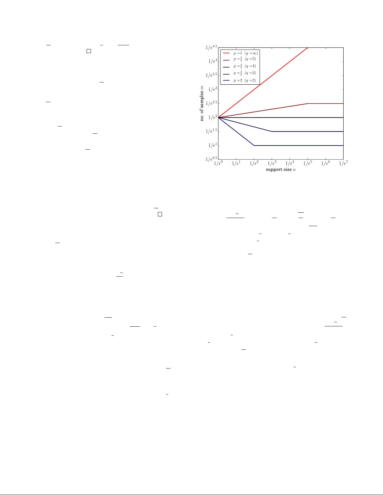
` p T esting and Learning of Discrete Distrib utions Bo W aggoner Har vard bwaggoner@f as .har vard.edu ABSTRA CT The classic problems of testing uniformity of and learning a discrete distribution, giv en access to indep endent samples from it, are examined under general ` p metrics. The intu- itions and results often contrast with the classic ` 1 case. F or p > 1 , we can learn and test with a n um b er of samples that is independent of the support size of the distribution: With an ` p tolerance  , O (max { p 1 / q , 1 / 2 } ) samples suﬃce for testing uniformit y and O (max { 1 / q , 1 / 2 } ) samples suﬃce for learning, where q = p/ ( p − 1) is the conjugate of p . As this parallels the in tuition that O ( √ n ) and O ( n ) samples suﬃce for the ` 1 case, it seems that 1 / q acts as an upp er bound on the “apparen t” supp ort size. F or some ` p metrics, uniformit y testing b ecomes easier ov er larger supp orts: a 6-sided die requires few er trials to test for fairness than a 2-sided coin, and a card-sh uﬄer requires few er trials than the die. In fact, this inv erse dependence on supp ort size holds if and only if p > 4 3 . The uniformit y testing algorithm simply thresholds the num b er of “collisions” or “coincidences” and has an optimal sample complexit y up to constan t factors for all 1 ≤ p ≤ 2 . Another algorithm giv es order-optimal sample complexit y for ` ∞ uniformit y testing. Mean while, the most natural learning algorithm is shown to ha ve order-optimal sample complexi ty for all ` p metrics. The author thanks Cl ´ emen t Canonne for discussions and con tributions to this work. This is the full ve rsion of the paper app earing at ITCS 2015. Categories and Subject Descriptors F.2.0 [ Analysis of Algorithms and Problem Complex- it y ]: general; G.3 [ Probabilit y and Statistics ]: proba- bilistic algorithms General T erms Algorithms, Theory Permission to make digital or hard copies of all or part of this work for personal or classroom use is granted without fee provided that copies are not made or distributed for proﬁt or commercial adv antage and that copies bear this notice and the full citation on the ﬁrst page. Copyrights for components of this work owned by others than the author(s) must be honored. Abstracting with credit is permitted. T o copy otherwise, or republish, to post on servers or to redistrib ute to lists, requires prior speciﬁc permission and/or a fee. Request permissions from permissions@acm.org. ITCS’15, January 11–13, 2015, Rehovot, Israel. Copyright is held by the owner/author(s). Publication rights licensed to ACM. A CM 978-1-4503-3333-7/15/01 ...$15.00. http://dx.doi.org/10.1145/2688073.2688095 . K eywords uniformit y testing; prop erty testing; learning; discrete distri- butions; lp norms 1. INTR ODUCTION Giv en indep enden t samples from a distribution, what w e can say ab out it? This question underlies a broad line of w ork in statistics and compu ter science. Speciﬁcally , w e w ould like algorithms that, giv en a small num b er of samples, can test whether some prop ert y of the distribution holds or can learn some attribute of the distribution. This paper considers tw o natural and classic examples. Uniformity testing asks us to decide, based on the samples w e ha ve drawn, whether the distribu tion is uniform ov er a domain of size n , or whether it is “  -far” from uniform according to some metric. Distribution le arning asks that, giv en our samples, w e output a sketc h or estimate that is within a distance  of the t rue distribution. F or both problems, w e would lik e to be correct except with some constan t probability of failure ( e.g. 1 3 ). The question studied is the num b er of indep endent samples required to solv e these problems. In practical applications we migh t imagine, such as a w eb compan y wishing to quic kly test or estimate the distribution of search keyw ords in a given day , the motiv ating goal is to formally guarantee go o d results while requiring as few samples as possible. Under the standard ` 1 distance metric (whic h is essentia lly equiv alent to total v ariation distance – we will use the term ` 1 only in this pap er), the question of uniformit y testing o ver large domain s was considered by P aninski [16], sho wing that Θ  √ n  2  samples are necessary and suﬃcien t for testing uniformity on supp ort size n , and it is known by “folklore” that Θ  n  2  samples are necessary and suﬃcien t for learning. Th us, these questions are settled 1 (up to constan t factors) if we are only in terested in ` 1 distance. Ho wev er, in testing and learning applications, w e may be in terested in other c hoices of metric than ` 1 . And more theoretically , w e might w onder whether the kno wn ` 1 b ounds capture all of the imp ortan t intuitions about the uniformity testing and distribution learning problems. Finally , we might lik e to understand our approaches for the ` 1 metric in a broader context or seek new tec hniques. This paper addresses these goals via ` p metrics. 1 [16] fo cused on the regime where supp ort size is very large, so order-optimal ` 1 uniformit y testing for the case of smaller n may ha ve been technically open prior to this work. 1.1 Motivations f or ` p Metrics In the survey “T aming Big Probabilit y Distributions” [17], Rubinfeld notes that ev en sublinear b ounds suc h as the abov e Θ  √ n  2  ma y still depend unacceptably on n , the supp ort size. If we do not ha ve enough samples, Rubinfeld suggests possible a ven ues suc h as assuming that the distribution in question has some v ery nice prop erty , e.g. monotonicit y , or assuming that the algorithm has the p ow er to make other t yp es of queries. Ho wev er, it is still possible to ask what can be done without suc h assumptions. One answ er is to consider what w e can sa y about our data under other measures of distance than the ` 1 distance. Do fewer samples suﬃce to draw conclusions? A primary implication of this pap er’s results is that this approac h do es succeed under general ` p metrics. The ` p distance betw een t wo probability distributions A, B ∈ R n for an y p ≥ 1, where A i is the probabilit y of drawing co ordinate i from distribution A , is the ` p norm of the v ector of diﬀerences in probabilities: k A − B k p = n X i =1 | A i − B i | p ! 1 /p . The ` ∞ distance is the largest diﬀerence of any coordinate, i.e. k A − B k ∞ = max i | A i − B i | . Unlik e the ` 1 case, it will turn out that for p > 1, w e can dra w conclusions ab out our data with a n um b er of samples that is indep endent of n and dep ends only on the desired error tolerance  . W e also ﬁnd smaller dep endences on the support size n ; in fact, for uniformit y testing we ﬁnd sometimes (p er- haps counte rintuitiv ely) that there is an inverse dep endence on n . The upshot is that, if we ha ve few samples, we may not b e able to conﬁdently solve an ` 1 testing or learning problem, but we ma y ha ve enough data to dra w conclusions about, say , ` 1 . 5 distance. This may also be useful in sa ying something about the ` 1 case: If the true distribution A has small ` 1 . 5 distance from our estimate ˆ A , yet actually does ha ve large ` 1 distance from ˆ A , then it must ha ve a certain shape ( e.g. large supp ort with many “light hitters” ). 2 Th us, this is the ﬁrst and primary motiv ation for the study of ` p metrics: to be able to dra w c onclusions with few samples but without making assumptions. A second motiv ation is to understand learning and testing under other ` p metrics for their own sake. In particular, the ` 2 and ` ∞ cases migh t b e considered imp ortant or fundamen tal. Ho wev er, even these are not alwa ys well understo o d. F or instance, “common knowledge” sa ys that Θ  1  2  samples are required to determine if one side of a coin is  -more lik ely to come up than it should be; one might naiv ely think that the same num b er of trials are required to test if an y card is  -more likely to be top in a shuﬄe of a sorted deck. But the latter can b e far less, as small as Θ  1   (depending on the relationship of  to the supp ort size), so a large improv ement is p ossible. Other ` p norms can also be of in terest when diﬀerent fea- tures of the distribution are of in terest. These norms trade oﬀ b etw een measuring the tail of the distribution ( p = 1 measures the total deviation even if it consists of man y tiny pieces) and measuring the he avy p ortion of the distribution ( p = ∞ measures only the single largest diﬀerence and ig- 2 I thank the anon ymous reviewers for suggesti ons and com- men ts regarding this motiv ation, including the ` 1 . 5 example. nores the others). Thus, an applica tion that needs to strike a balance ma y ﬁnd that it is b est to test or estimate the distri- bution under the particular p that optimizes some tradeoﬀ. General ` p norms, and especially ` 2 and ` ∞ , also can ha ve immediate applications tow ard testing and learning other properties. F or instance, [1] developed and used an ` 2 tester as a blac k box in order to test the ` 1 distance betw een t wo distributions. Utilizing a b etter ` 2 tester (for instance, one immediately deriv ed from the learner in this pap er) leads to an immediate improv ement in the samples required by their algorithm for the ` 1 problem. 3 A third motiv ation for ` p testing and learning, b eyond dra wing conclusions from less data and indep endent inter- est/use, is to develo p a deeper understanding of ` p spaces and norms in relation to testing and learning problems. Perhaps tec hniques or ideas developed for addressing these problems can lead to more simple, general, and/or sharp approac hes in the sp ecial ` 1 case. More broadly , learning or sketc hing general ` p v ectors hav e many important applications in set- tings such as mac hine learning ( e.g. [13]), are of independent in terest in settings suc h as streaming and sketc hing ( e.g. [12]), and are a useful to ol for estimating other quan tities ( e.g. [5]). Improv ed understandings of ` p questions ha v e b een used in the past to shed new ligh t on w ell-studied ` 1 problems [14]. Th us, studying ` p norms in the context of learning and testing distributions ma y provide the opportunity to app ly , reﬁne, or dev elop techniques relev an t to these areas. 1.2 Organization The next section summarizes the results and describ es some of the k ey in tuitions/conceptual tak eaw ays from this w ork. Then, we will describ e the results and techniqu es for the uniformit y testing problem, and then the learning problem. W e then conclude b y discussing the broader con text, prior w ork, and future work. Most pro ofs are omitted in the b o dy of the pap er (though sk etches are usually provided). There is attached an app endix con taining all pro ofs. 2. SUMMAR Y AND KEY THEMES A t a technical level, this pap er prov es upper and low er b ounds for num b er of samples required for testi ng uniformity and learning for ` p metrics. These problems are formally deﬁned as follo ws. F or eac h problem, w e are given i.i.d. sam- ples from a distribution A on supp ort size n . The algorithm m ust sp ecify the n umber of samples m to dra w and satisfy the stated guaran tees. Uniformit y testing: If A = U n , the uniform distribution on supp ort size n , then output “uniform” . If k A − U n k p ≥  , then output “not uniform” . In each case, the output must be correct except with some constant failure probability δ ( e.g. δ = 1 3 ). Learning: Output a distribution ˆ A satisfying that k A − ˆ A k p ≤  . This condition m ust b e satisﬁed except with some constan t failure probabilit y δ ( e.g. δ = 1 3 ). In both cases, the algorithm is given p, n, , δ . Summar y Theorem 1. F or the pr oblems of testing uni- formity of and le arning a distribution, the numb er of samples ne c essary and suﬃcient satisfy, up to c onstant factors de- p ending on p and δ , the bound s in T able 1. 3 F urther impro v ement for this problem is ac hieved in [4]. In p articular, for e ach ﬁxe d ` p metric and failur e pr ob ability δ , the upp er and lower b ounds match up to a c onstant factor for distribution le arning for all p ar ameters and for unifo rmity testing when 1 ≤ p ≤ 2 , when p = ∞ , and when p > 2 and n is “lar ge” ( n ≥ 1  2 ). T able 1 is in tended as a reference and summary; the reader can safely skip it and read on for a description and explana- tion of the key themes and results, after whic h (it is hop ed) T able 1 will be more comprehensible. Later in the paper, we give more speciﬁc theorems con- taining (small) explicit constan t factors for our algorithms. Some of these bounds are new and emplo y new tec hniques, while others are either already known or can b e deduced quic kly from known bounds; discussion fo cuses on the nov el aspects of these results and Section 6 describes the relation- ship to prior w ork. The remainder of this section is dev oted to highlighting the most important themes and conceptually imp ortan t or surprising results (in the author’s opinion). The following sections detail the tec hniques and results for the uniformity testing and learning problems respectively . 2.1 Fixed bounds f or large n r egimes A primary theme of the results is the in tuition b ehind ` p testing and learning in the case where the support size n is large. In ` p spaces for p > 1, we can ac hiev e upp er bounds for testing and learning that are independent of n . Summar y Theorem 2. F or a ﬁxe d p > 1 , let q be the H ¨ older c onjugate 4 of p with 1 p + 1 q = 1 . Let n ∗ = 1 / q . Then O  max  √ n ∗ , 1  2  samples ar e suﬃcient for testing uniformity and O  max  n ∗ , 1  2  ar e suﬃcient for le arning. F urthermor e, for 1 < p ≤ 2 , when the supp ort size n exc e e ds n ∗ , then Θ  √ n ∗  and Θ ( n ∗ ) r esp e ctively ar e ne c essary and suﬃcient. In tuitively , particularly for 1 < p ≤ 2, w e can separate in to “large n ” and “small n ” regimes 5 , where the divider is n ∗ = 1  q . In the small n regime, tight b ounds depend on n , but in the large n regime where n ≥ n ∗ , the num b er of samples is Θ ( n ∗ ) for learning and Θ  √ n ∗  for uniformit y testing. This suggests the in tuition that, in ` p space with tolerance  , distributions’ “ap parent” support sizes are b ounded by n ∗ = 1  q . W e next mak e tw o observ ations that align with this persp ective, for purposes of intuition. Obser v a tion 2.1. L et 1 < p and q = p p − 1 . If the distri- bution A is “thin ” in that max i A i ≤  q , then k A k p ≤  . In p articular, if b oth distributions A and B ar e thin, then even if they ar e c ompletely disjoint, k A − B k p ≤ k A k p + k B k p ≤ 2 . Proof. The claim holds immediately for p = ∞ . F or 1 < p < ∞ , by conv exity , since P i A i = 1 and max i A i ≤  q , we hav e that k A k p p = P i A p i is maximized with as few nonzero entries as p ossible, each at its maximum v alue  q . 4 Note that 1 and ∞ are considered conjugates. This pap er will also use math with inﬁnit y , so for instance, when q = ∞ , n 1 /q = 1 and it is never the case that n ≤ 1  q . 5 F or p ≥ 2, this separation still makes sense in certain w ays (see Observ ations 2.1 and 2.2 b elow ) but do es not appear in the sample complexit y b ounds in this paper. Learning for 1 ≤ p ≤ 2 : regime n ≤ 1  q n ≥ 1  q necessary and suﬃcien t n ( n 1 /q  ) 2 1  q Uniformit y testing for 1 ≤ p ≤ 2 : regime n ≤ 1  q n ≥ 1  q necessary and suﬃcien t √ n ( n 1 /q  ) 2 q 1  q Learning for 2 ≤ p ≤ ∞ : 1  2 (necessary and suﬃcien t, all regimes). Uniformit y testing for p = ∞ : regime Θ  n ln( n )  ≤ 1  1  ≤ Θ  n ln( n )  necessary and suﬃcien t ln( n ) n 2 1  Uniformit y testing for 2 < p < ∞ : regime Θ  n ln( n )  ≤ 1  1  ≤ Θ  n ln( n )  , n ≤ 1  2 n ≥ 1  2 necessary ln( n ) n 2 1  1  suﬃcien t 1 √ n 2 1 √ n 2 1  T able 1: Results summary . In eac h problem, w e are giv en independent samples from a distribution on supp ort size n . Eac h entry in the tables is the num b er of samples drawn necessary and/or suﬃcien t, up to constan t factors dep ending only on p and the ﬁxed probability of failure. Throughout the paper, q is the H ¨ older conjugagte of p , with q = p p − 1 (and q = ∞ for p = 1). In uniformity testing , we m ust decide whether the distribu- tion is U n , the uniform distribution on support size n , or is ` p distance at least  from U n . [16] gav e the optimal upper and lo w er bound in the case p = 1 (with unkno wn constan ts) for large n ; other results are new to my kno wledge. In le arning , we m ust output a distribution at ` p distance at most  from the given distribution, which has support size at most n . Optimal upp er and low er b ounds for learning in the cases p = 1, 2, and ∞ seem to the author to be all previously kno wn as folklore (certainly for ` 1 and ` ∞ ); others are new to my knowledge. This extreme example is simply the uniform distribution on n = 1  q , when k A k p p = n  1 n  p = 1 n p − 1 =  . The rest is the triangle inequalit y . One takea wa y from Observ ation 2.1 is that if we are in ter- ested in an ` p error tolerance of Θ (  ) , then an y suﬃcien tly “thin” distribution may almost as well b e the uniform dis- tribution on support size 1  q . This p ersp ectiv e is reinforced b y Observ ation 2.2, whic h says that under the same circum- stances, any distributio n may almost as well be “discretized” in to 1  q c hunks of w eigh t  q eac h. Obser v a tion 2.2. Fixing 1 < p , for any distribution A , ther e is a distribution B whose pr ob abilities ar e inte ger mul- tiples of 1  q such that k A − B k p ≤ 2  . In p articular, B ’s supp ort size is at most 1  q . Proof. W e can alw ays c hoose B suc h that, on each coor- dinate i , | A i − B i | ≤ 1  q . (T o see this, obtain the v ector B 0 b y rounding eac h coordinate of A up to the nearest in teger mul- tiple of  q , and obtain B 00 b y rounding each coordinate do wn. k B 0 k 1 ≥ 1 ≥ k B 00 k 1 , so we can obtain a true probabilit y dis- tribution by taking some coordinates from B 0 and some from B 00 .) But this just sa ys that the v ector A − B is “thin” in the sense of Observ ation 2.1. The same argumen t go es through here (ev en though A − B is not a probabilit y distribution): Since max i | A i − B i | ≤  q and P i | A i − B i | ≤ 2, b y con v exity k A − B k p is maximized when it has dimension 2  q and eac h en try | A i − B i | =  q , so we get k A − B k p ≤ 2  . 2.2 T esting unif ormity: biased coins and die Giv en a coin, is it fair or  -far from fair? It is well-kno wn that Ω  1  2  independent ﬂips of the coin are necessary to mak e a determination with conﬁdence. One migh t naturally assume that deciding if a 6-sided die is fair or  -far from fair w ould only be more diﬃcult, requiring more rolls, and one w ould b e correct — if the measure of “  -far” is ` 1 distance. Indeed, it is known [16] that Θ  √ n  2  rolls of an n -sided die are necessary if the auditor’s distance measure is ` 1 . But what ab out other measures, say , if the auditor wishes to test whether any one side of the die is  more lik ely to come up than it should be? F or this ` ∞ question, it turns out that fewer rolls of the die are required than ﬂips of the coin; speciﬁcally , w e show that Θ  ln n n 2  are necessary and suﬃcient, in a small n regime (sp eciﬁcally , Θ  n ln( n )  ≤ 1  ). Once n b ecomes large enough, only Θ  1   samples are necessary and suﬃcien t. Brieﬂy , the in tuition b ehind this result in the ` ∞ case is as follo ws. When ﬂipping a 2-sided coin, both a fair coin and one that is  -biased will ha ve man y samples that are heads and man y that are tails, making  diﬃcult to detect ( 1  2 ﬂips are needed to ov ercome the v ariance of the pro cess). On the other hand, imagine that w e roll a die with n =one million faces, for which one particular face is  = 0 . 01 more likely to come up than it should b e. Then after only Θ  1   = a few hundred rolls of the die, we expect to see this face come up multiple times. These multiple-occurrences or “collisions” are v astly less likely if the die is fair, so w e can distinguish the biased and uniform cases. So when the supp ort is small, the v ariance of the uniform distribution can mask bias; but this fails to happen when the support size is large, making it easier to test uniformity o ver larger supports. These intuitions extend smoothly to the ` p 1 / 0 1 / 1 1 / 2 1 / 3 1 / 4 1 / 5 1 / 6 1 / 7 support size n 1 / 0 . 5 1 / 1 1 / 1 . 5 1 / 2 1 / 2 . 5 1 / 3 1 / 3 . 5 1 / 4 1 / 4 . 5 no . of samples m p =1 ( q = ∞ ) p = 5 4 ( q =5) p = 4 3 ( q =4) p = 3 2 ( q =3) p =2 ( q =2) Figure 1: Samples (necessary and suﬃcien t, up to constan t factors) for testing uniformit y with a ﬁxed ` p tolerance  . On the horizon tal axis is the sup p ort size n of the uniform distribution, and on the vertical axis is the corresponding n umber of samples required to test uniformit y . The function plotted is √ n ( n 1 /q  ) 2 for n ≤ 1  q and q 1  q for n ≥ 1  q , for v arious choices of p and corresp onding q = p p − 1 . There is a phase transition at p = 4 3 : F or p < 4 3 , the bound is initially increasing in n ; for p > 4 3 , the bound is initially decreasing in n . F or all p except p = 1, the n umber of necessary samples is constan t for n ≥ 1  q . Note the log-log scale. metrics below p = ∞ : First, to b e  -far from uniform on a large set, it m ust b e the case that the distribution has “heavy” elemen ts; and secon d, these heavy elemen ts cause many more collisions than the uniform distribution, making them easier to detect than when the supp ort is small. Ho wev er, this in tuition only extends “down” to certain v alues of p . Summar y Theorem 3. F or 1 ≤ p ≤ 2 , for n ≤ n ∗ = 1  q , the sample c omplexity of testing uniformity is Θ  √ n ( n 1 /q  ) 2  . F or 1 ≤ p < 4 3 , this is incre asing in the supp ort size n , and for 4 3 < p ≤ 2 , this is de cr eas ing in n . F or p = 4 3 , the sample c omplexity is Θ  1  2  for every value of n . Figure 1 illustrates these bounds for diﬀerent v alues of p , including the phase transition at p = 4 3 . 3. UNIFORMITY TESTING FOR 1 ≤ p ≤ 2 Recall the deﬁnition of uniformity testing: giv en i.i.d. samples from a distribution A , w e must satisfy the follo wing. If A = U n , the uniform distribution on support size n , then with probability at least 1 − δ , output “u niform” . If k A − U n k p ≥  , then with probabilit y at least 1 − δ , output “not uniform” . Algorithm 1 Uniformity T ester On input p, n,  , and failur e pr ob ability δ : Choose m to be “ suﬃcien t” for p, n, , δ according to pro ven bounds. Dra w m samples. Let C b e the num b er of collisions: C = P 1 ≤ j T , output “not uniform” . The upp er b ounds for 1 ≤ p ≤ 2 rely on a v ery simple algorithm, Algorithm 1, and straightforw ard (if slightly deli- cate) argumen t. W e coun t the num ber of c ol lisions : Pairs of samples drawn that are of the same co ordinate. (Thus, if m samples are dra wn, there are up to  m 2  possible collisions.) The n umber of collisions C has the following properties. 6 Lemma 3.1. On distribution A , the numb er of c ol lisions C satisﬁes: 1. The exp e ctation is µ A =  m 2  k A k 2 2 =  m 2   1 n + k A − U k 2 2  . 2. The varianc e is V ar ( C ) =  m 2   k A k 2 2 − k A k 4 2  + 6  m 3   k A k 3 3 − k A k 4 2  . Th us, the ` 2 distance to uniform, k A − U k 2 , in tuitively con trols the num b er of collisions we expect to see, with a minim um when A = U . This is why Algorithm 1 simply de- clares the distribution nonuniform if the n um b er of collisions exceeds a threshold. Theorem 3.1. F or uniformity testing with 1 ≤ p ≤ 2 , it suﬃc es to run Algorithm 1 while dr awing the fol lowing numb er of samples: m = 9 δ        √ n ( n 1 /q ) 2 n ≤ 1  q 1 2 q  2   q n ≥ 1  q . The proof of Theorem 3.1 uses Cheb yshev’s inequality to bound the probability that C is far from its exp ectation in terms of V ar ( C ), for b oth the case where A = U n and k A − U n k p ≥  . It focuses on a careful analysis of the v ariance of the n umber of collisions, to sho w that, for m suﬃcien tly large, the v ariance is small. F or 1 ≤ p ≤ 2, the dominan t term ev entually falls into one of tw o cases, whic h corresp ond directly to “large n ” ( n ≥ 1  q ) and “small n ” ( n ≤ 1  q ). 6 A p ossibly in teresting generalization: The expected num b er of k -wa y collisions, for any k = 2 , 3 , . . . , is equal to  m k  k A k k k . T o pro ve it, conside r the probabilit y that eac h k -sized subset is suc h a collision ( i.e. all k are of the same co ordinate), and use linearit y of exp ectation o ver the  m k  subsets. Collisions, also called “coincidences” , ha ve been implicitly , but not explicitly , used to test uniformity for the ` 1 case b y Paninski [16]. Rather than directly testing the num b er of collisions, that paper tested the num b er of co ordinates that were sampled exactl y once. That tester is designed for the regime where n > m . Collisions hav e also b een used for similar testing problems in [11, 1]. One in teresting note is that T is deﬁned in terms of m , so that no matter ho w m is c hosen, if A = U then the algorithm outputs “uniform” with probabilit y 1 − δ . W e also note that, if very high conﬁdence is desired, a logarithmic dep endence on δ is achiev able by rep eatedly running Algorithm 1 for a ﬁxed failure probabilit y and taking a ma jorit y v ote. The constan ts in the Theorem 3.2 are chosen to optimize the n umber of samples. Theorem 3.2. F or uniformity testing with 1 ≤ p ≤ 2 , it suﬃc es to run Algorithm 1 160 ln (1 /δ ) / 9 times, e ach with a ﬁxe d failur e pr ob ability 0 . 2 , and output ac c or ding to a majority vote; thus dr awing a total numb er of samples m = 800 ln(1 /δ )        √ n ( n 1 /q ) 2 n ≤ 1  q 1 2 q  2   q n ≥ 1  q . This impr oves on The or em 3.1 when the failur e pr ob ability δ ≤ 0 . 002 or so. The follo wing lo wer b ound sho ws that Algorithm 1 is optimal for all 1 ≤ p ≤ 2, n , and  , up to a constant factor depending on p and the failure probability δ . Theorem 3.3. F or uniformity testing with 1 ≤ p ≤ 2 , it is nec essary to dr aw the fol lowing numb er of samples: m =      p ln (1 + (1 − 2 δ ) 2 ) √ n ( n 1 /q ) 2 n ≤ 1  q p 2(1 − 2 δ ) q 1 (2  ) q n ≥ 1  q . In the large- n regime, the low er b ound can b e prov en sim- ply . W e pic k randomly from a set of nonuniform distributions A where, if not enough samples are dra wn, then the proba- bilit y of any collision is v ery lo w. But without collisions, the input is equally likely to come from U n or from one of the non uniform A s, so no algorithm can distinguish these cases. In the small- n regime, the order-optimal low er bound follo ws from the ` 1 lo wer bound of Pa ninski [16], which do es not give constants. W e giv e a rewriting of this pro of with t wo changes: W e make small adaptations to ﬁt general ` p metrics, and we obtain the constan t factor. The idea b ehind the proof of [16] is to again pick randomly from a family of distributions that are close to uniform. It is sho wn that any algorithm’s probabilit y of success is b ounded in terms of the distance from the distribution of the resulting samples to that of samples dra wn from U n . 4. UNIFORMITY TESTING FOR p > 2 This pap er fails to characterize the sample complexity of uniformity testing in the p > 2 regime, except for the case p = ∞ in which the bounds are tigh t. Ho wev er, the remaining gap is relativ ely small. First, we note that Algorithm 1 can b e slightly adapted for use for all p > 2, giving an upper b ound on the n um b er of samples required. The reason is that, by an ` p -norm inequalit y , whenev er k A − U k p ≥  , w e also hav e k A − U k 2 ≥  . So an ` 2 tester is also an ` p tester for p ≥ 2. This observ ation pro ves the follo wing theorem. Theorem 4.1. F or uniformity testing with any p > 2 , it suﬃc es to run Algorithm 1 while dr awing the numb er of samples for p = 2 fr om Theo r em 3.1, namely m = 9 δ    1 √ n 2 n ≤ 1  2 1  n ≥ 1  2 . (A lo garithmic dep endenc e on δ is also p ossible as in The or em 3.2.) Proof. If A = U , then b y the guarantee of Algorit hm 1, with probabilit y 1 − δ it outputs “uniform” . If k A − U k p ≥  , then k A − U k 2 ≥  : It is a prop erty of ` p norms that k V k 2 ≥ k V k p for all vectors V when p ≥ 2. Then, by the guaran tee of Algorithm 1, with probabilit y 1 − δ it outputs “not uniform” . The same reasoning, but in the opposite direction, sa ys that a low er bound for the ` ∞ case gives a low er b ound for all p < ∞ . Thus, b y proving a lo wer bound for ` ∞ distance, we obtain the follo wing theorem. Theorem 4.2. F or uniformity testing with any p , it is ne c essary to dr aw the fol lowing numb er of samples: m =      1 2 ln ( 1+ n (1 − 2 δ ) 2 ) n 2 for al l n 1 − 2 δ 2 1  n ≥ 1  . We ﬁnd that the ﬁrst b ound is lar ger (b etter) for Θ  n ln( n )  ≤ 1  , and the se c ond is b etter for al l larg er n . Proof. In the appendix (Theorems C.1 and C.2), it is pro ven that this is a low er-b ound on the n umber of samples for the case p = ∞ . B y the p -norm inequality mentioned abov e, for any p ≤ ∞ and any v ector V , k V k p ≥ k V k ∞ . In particular, suppose we had an ` p testing algorithm. When the sampling distribution A = U n , then by the guarantee of the ` p tester it is correct with probabilit y at least 1 − δ ; when k A − U n k ∞ ≥  , we m ust ha ve k A − U n k p ≥  and so again b y the guaran tee of the ` p tester it is correct with probabilit y 1 − δ . Thus the low er bound for ` ∞ holds for any ` p algorithm as w ell. The lo wer bound for ` ∞ distance is prov en b y again splitting in to the large and small n cases. In the large n case, w e can simply consider the distribution A ∗ =  1 n + , 1 n −  n − 1 , . . . , 1 n −  n − 1  . If m is too small, then the algorithm probably does not draw an y sample of the ﬁrst coordinate; but conditioned on this, A ∗ is indistinguishable from uniform (since it is uniform on the remaining coordinates). In the small n case, we adapt the general approac h of [16] that w as used to pro ve tigh t lo w er b ounds for the case p ≤ 2. W e consider c ho osing a random p ermutation of A ∗ and then dra wing m i.i.d. samples from this distribution. As b efore, w e b ound the success probabilit y of any algo rithm in terms of the distance betw een the distribution of these samples and that of the samples from U n . Comparing Theorems 4.1 and 4.2, w e see a relatively small gap for the small n regime for 2 < p < ∞ , which is left op en. A natural conjecture is that the sample complexity will b e 1  for the regime n ≥ 1  q . F or the small n regime, it is not clear what to exp ect; perhaps 1 n 1 /q  2 . New techniques seem to be required, since neither the analysis of collisions as in the case p ≤ 2, nor the analysis of the single most diﬀerent coordinate, as we will see for the p = ∞ case below, seems appropriate or tigh t for the case 2 < p < ∞ . A b etter ` ∞ tester. F or the ` ∞ case, the ` 2 tester is optimal in the regime where n ≥ 1  2 , as pro ven in Theorem 4.1. F or smaller n , a natural algorithm (alb eit with some tric ky sp eciﬁcs), Algorithm 2, gives an upp er b ound that matc hes the low er b ound up to constant factors. W e ﬁrst state this upper b ound, then explain. Theorem 4.3. F or uniformity testing with ` p distanc e, it suﬃc es to run Algorithm 2 with the fol lowing numb er of samples: m =      23 ln ( 2 n δ ) n 2  ≤ 2 α ( n ) 35 ln ( 1 δ )   > 2 α ( n ) wher e α ( n ) = 1 n  1 + ln(2 n ) ln(1 /δ )  . In p articular, for a ﬁxe d failur e pr ob ability δ , we have α ( n ) = Θ  ln( n ) n  . T o understand Algorithm 2, consider separately the t w o regimes: Θ  n ln( n )  ≤ 1  and otherwise. F or details of the analysis, rather than phrasing the threshold in this wa y , we phrase it as  ≤ 2 α ( n ) where α ( n ) = Θ  ln( n ) n  , but the actual form of α is more complicated b ecause it dep ends on δ . In the ﬁrst, smaller- n regime, our approac h will essentially b e a Che rnoﬀ plus union bound. W e will draw m = Θ  ln( n ) n 2  samples. Then Algorithm 2 simply c hecks for an y coordinate with an “outlier” num b er of samples (either too many or too few). The pro of of correctness is that, if the distribution is uniform, then b y a Chernoﬀ bound on each co ordinate and union-bound ov er the co ordinates, with high probabilit y no co ordinate has an “outlier” n um b er of samples; on the other hand, if the distribution is non-uniform, then there is an “outlier” coordinate in terms of its probabilit y and b y a Chernoﬀ bound this coordinate lik ely has an “outlier” nu mber of samples. In the second, larger- n regime (where  > 2 α ( n )), we will use the same approac h, but ﬁrst w e will “ buck et” the distribution in to ˆ n groups where ˆ n is c hosen suc h that  = 2 α ( ˆ n ). In other words, no matter ho w large n is, w e choose ˆ n so that  = Θ  ln( ˆ n ) ˆ n  and treat each of the ˆ n groups as its o wn co ordinate, counting the n um b er of samples that group gets. In this larger- n regime, note that  is large compared to the probabilit y that the uniform distribution puts on each coordinate, or in fact on each group. So if k A − U k ∞ ≥  , then there is a “heavy” co ordinate (and th us group containing it) that should get an outlier num b er of samples. W e also need, b y a Chernoﬀ plus union b ound, that under the uniform distribution, probably no group is an outlier. The key point of our choice of ˆ n is that it exactly balances this Chernoﬀ plus union bound. Algorithm 2 Uniformity T ester for ` ∞ On input n,  , and failur e pr ob ability δ : Choose m to b e “suﬃcien t” for n, , δ according to prov en bounds. Dra w m samples. Let α ( x ) = 1 x  1 + ln(2 x ) ln(1 /δ )  = Θ  ln( x ) x  . if  ≤ 2 α ( n ) then Let t = q 6 m n ln  2 n δ  . If, for all co ordinates i , the num b er of samples X i ∈ m n ± t , output “uniform” . Otherwise, output “not uniform” . else Let ˆ n satisfy  = 2 α ( ˆ n ). P artition the co ordinates into at most 2 d ˆ n e groups, eac h of size at most b n ˆ n c . F or eac h group j , let X j b e the tot al n umber of samples of coordinates in that group. Let t = q 6 m ln  1 δ  . If there exists a group j with X j ≥ m − t , output “not uniform” . Otherwise, output “uniform” . end if 5. DISTRIBUTION LEARNING Recall the deﬁnition of the learning proble m: Given i.i.d. samples from a distribution A , w e m ust output a distribution ˆ A satisfying that k A − ˆ A k p ≤  . This condition must be satisﬁed except with probabilit y at most δ . 5.1 Upper Bounds Here, Algorithm 3 is the natural/naive one: Let the prob- abilit y of each coordinate be the frequency with which it is sampled. Algorithm 3 Learner On input p, n,  , and failur e pr ob ability δ : Choose m to be “ suﬃcien t” for p, n, , δ according to pro ven bounds. Dra w m samples. Let X i b e the num ber of samples drawn of each coordinate i ∈ { 1 , . . . , n } . Let eac h ˆ A i = X i m . Output ˆ A . The proofs of the upp er bounds rely on an elegan t pro of approac h whic h is apparently “folklore” or known for the ` 2 setting, and was introduced to the author by Cl´ emen t Canonne[3] who con tributed it to this paper. The author and Canonne in collaboration extended the proof to general ` p metrics in order to pro ve the bounds in this pap er. Here, w e giv e the theorem and proof for p erhaps the most interesting and nov el case, that for 1 < p ≤ 2, O  1  q  samples are suﬃcien t indep enden t of n . The other cases ha ve a simila r proof structure. Theorem 5.1. F or 1 < p ≤ 2 , to le arn up to ` p distanc e  with failur e pr ob ability δ , it suﬃc es to run Algori thm 3 while dr awing the fol lowing numb er of samples: m =  3 δ  1 p − 1 1  q . Proof. Let X i be the num b er of samples of coordinate i and ˆ A i = X i m . Note that X i is distributed Binomially with m independent trials of probabilit y A i eac h. W e ha ve that E k ˆ A − A k p p = 1 m p n X i =1 E | X i − E X i | p . W e will sho w that, for each i , E | X i − E X i | p ≤ 3 E X i . This will complete the proof, as then E k ˆ A − A k p p ≤ 1 m p n X i =1 3 E X i = 1 m p n X i =1 3 mA i = 3 m p − 1 ; and b y Marko v’s Inequality , Pr[ k ˆ A − A k p p ≥  p ] ≤ 3 m p − 1  p , whic h for m =  3 δ  1 p − 1 1  q is equal to δ . T o sho w that E | X i − E X i | p ≤ 3 E X i , ﬁx any i and con- sider a possible realization x of X i . If | x − E X i | ≥ 1, then | x − E X i | p ≤ | x − E X i | 2 . W e can t hus b ound the con tribution of all suc h terms by E | X i − E X i | 2 = V ar X i . If, on the other hand, | x − E X i | < 1, then | X i − E X i | p ≤ | X i − E X i | ; furthermore, at most tw o terms satisfy this condition, namely (letting β := b E X i c ) x = β and x = β + 1. These terms con tribute a total of at most Pr[ X i = β ] | E X i − β | + Pr[ X i = β + 1] | β + 1 − E X i | ≤ E X i + Pr[ X i = β + 1] . Consider tw o cases. If E X i ≥ 1, then the contribution is at most E X i + 1 ≤ 2 E X i . If E X i < 1, then β + 1 = 1, and by Mark ov’s Inequalit y , Pr [ X i ≥ 1] ≤ E X i , so the total con tribution is again b ounded b y 2 E X i . Th us, we ha v e E | X i − E X i | p ≤ V ar X i + 2 E X i ≤ 3 E X i because V ar X i = (1 − A i ) E X i . A sligh tly tighter analysis can b e obtained by reducing to the ` 2 algorithm, in which the ab ov e pro of technique is “tigh test” . It pro duces the following theorem: Theorem 5.2. F or learning a discr ete distribution with 1 ≤ p ≤ 2 , it suﬃc es to run Algorithm 3 with the fol lowing numb er of samples: m = 1 δ    n ( n 1 /q  ) 2 n ≤  2   q 1 4  2   q n ≥  2   q . With p ≥ 2 , it suﬃc es to dr aw the suﬃcient numb er for ` 2 le arning, namely m = 1 δ 1  2 . In fact, k A − ˆ A k p is tightly concen trated around its ex- pectation, allowing a b etter asymptotic dep endence on δ when high conﬁdence is desired. This idea is also folklore and not original to this pap er. Here we apply it as follows. W e m ust draw eno ugh samples so that, ﬁrst, the exp ectation of k ˆ A − A k p is smaller than  2 ; and second, we must draw enough so that, with probability 1 − δ , k ˆ A − A k p is no more than  2 greater than its expectation. It suﬃces to take the maxim um of the num b er of samples that suﬃce for each condition to hold, resulting in the follo wing b ounds. Theorem 5.3. F or learning a discr ete distribution with 1 ≤ p ≤ 2 and failur e pr ob ability δ , it suﬃc es to run Algo- rithm 3 with the fol lowing numb er of samples: m = max ( 2 2 p +1 ln(1 /δ )  2 , M ) , wher e M =    4 n ( n 1 /q  ) 2 n ≤  4   q 1 4  4   q n ≥  4   q . F or p ≥ 2 , it suﬃc es to use the suﬃc ent numb er of samples for ` 2 le arning, namely m = max  4 ln(1 /δ )  2 , 4  2  . In particular, for ` 1 learning, it suﬃces to dra w m = max  8 ln(1 /δ )  2 , 4 n  2  . 5.2 Lower bounds Theorem 5.4. T o le arn a discr ete distribution in ` p dis- tanc e, the numb er of samples r e quir e d for al l p, δ is at le ast m =    Ω  1  2  2 ≤ p ≤ ∞ Ω  1  q  1 < p ≤ 2 , n ≥ 1  q . F or 1 ≤ p ≤ 2 and n ≤ 1  q , there is no γ > 0 such that m = O n ( n 1 /q  ) 2 − γ ! samples, up to a c onstant factor dep ending on δ , suﬃc e for al l δ . As detailed in App endix D.2, these b ounds can be pro ven from the folklore ` 1 bound for the case 1 ≤ p ≤ 2 (which seems to giv e a slightly tigh ter guarantee than the theorem statemen t); and the lo wer b ound for ` ∞ uniformit y testing giv es the tigh t b ound for 2 ≤ p ≤ ∞ . Finding it somewhat unsatisfying to reduce to the ` 1 folklore result, w e attempt an independent proof. This approach will giv e tight bounds up to (unspeciﬁed) constant factors for all p and δ in the 1 < p ≤ 2, “large n ” ( n ≥ 1  q ) regime. In the small n regime, w e will get b ounds that lo ok like n ( n 1 /q  ) 2(1 − δ ) instead of n ( n 1 /q  ) 2 (in terpreted as in the ab ov e theorem). Thus, in this paper, the low er b ound for this regime matches the upp er b ound in a w eak sense; it would be nice if the below appro ach can be impro ved to yield a stronger statemen t. W e begin by deﬁning the follo wing game and proving the associated lemma: Distribution identiﬁcation game: The game is parame- terized b y maximum support size n , distance metric ρ , and tolerance  . First, a ﬁnite set S of distributions is chos en with ρ ( A, B ) > 2  for all A, B ∈ S . Every dist ribution in S has support ˆ n ≤ n (it will be useful to c ho ose ˆ n 6 = n ). The algorithm is giv en S . Second, a distributio n A ∈ S uniformly at random. Third, the algorithm is given m i.i.d. samples from A . F ourth, the algorithm wins if it correctly guesses whic h A ∈ S was c hosen, and loses otherwise. Lemma 5.1. An y algorithm for le arning to within distanc e  using m ( n, p,  ) samples with failur e pr ob ability δ c an b e c onverte d into an algorithm for distribution identiﬁc ation using m ( n, p,  ) samples, with losing pr ob ability at most δ . Proof. Suppose the true oracle is A ∈ S . Run the learn- ing algorithm, obtaining ˆ A , and output the mem b er B of S that minimizes ρ ( ˆ A , B ) (where ρ is the distance metric of the game; for us, it will b e ` p distance). With probabilit y at least 1 − δ , by the guarantee of the learning algorithm, k ˆ A − A k p ≤  . When this o ccurs, we alwa ys output the correct answer, A : F or any B 6 = A in S , by the triangle inequalit y k ˆ A − B k p ≥ k B − A k − k ˆ A − A k > 2  −  =  . The proofs of the lo wer b ounds then proceed in the follo w- ing fashion, at a high lev el: 1. Construct a large set S of distributions. F or instance, for 1 ≤ p ≤ 2, we hav e | S | ≈  1 ( ˆ n ) 1 /q   ˆ n . The main idea is to use a sphere-packing argumen t as with e.g. the Gilb ert-V arshamo v b ound in error-correcting co des. (In particular, the “construction” is not constructive; w e merely prov e that suc h a set exists.) 2. Relate the probabilit y of winning the game to the information obtained from the samples. Intuitiv ely , w e need a go o d ratio of the entrop y of the samples, ≈ ˆ n log  p m ˆ n  , to the entrop y of the choice of distribu- tion, log | S | . 3. Com bine these steps. F or instance, for 1 ≤ p ≤ 2, w e get that the probability of winning lo oks lik e  ˆ n 1 /q  p m ˆ n  ˆ n , implying that, for a constan t probability of winning, w e must pic k m ≈ ˆ n (( ˆ n ) 1 /q  ) 2 . 4. Choose ˆ n ≤ n . F or 1 ≤ p ≤ 2, in the small n regime where n ≤ 1  q , the b est c hoice turns out to b e ˆ n = n ; in the large n regime, the choice ˆ n = 1  q turns out to b e optimal and gives a low er b ound Θ ( ˆ n ) that is independent of n for that range (since for any large enough n , w e make the same c hoice of ˆ n ). 6. PRIOR AND FUTURE WORK 6.1 Discussion of Prior W ork The study of problems under ` p metrics crops up in many areas of theoretical computer science and probabilit y , as men- tioned in the introduction. Similar in spirit to this pap er is Berman et al 2014 [2], which examined testing properties of real-v alued functions such as monotonicit y , Lipsc hitz con- stan t, and conv exity , all under v arious ` p distances. Another case in which “ exotic” metrics hav e been studied in connection with testing and learning is in Do et al 2011 [9], whic h studied the distance betw een and equalit y of t wo distributions under Earth Mo ver Distance. F or the problem of testing uniformit y , Paninski 2008 [16] examines the ` 1 metric in the case of large-supp ort distribu- tions. The lo wer b ound tec hnique, which is sligh tly extended and utilized in this pap er, establishes that Ω  √ n  2  samples are necessary to test uniformity under the ` 1 metric (with constan ts unknown). This low er b ound holds for all supp ort sizes n . The algorithm that gives the upper b ound in that paper, a matching m = O  √ n  2  , holds for the case of very large supp ort size n , namely n > m . This translates to n = Ω  1  4  . The reason is that the algorithm counts the n umber of co ordinates that are sampled exactly once; when n > m , this indirectly counts the num b er of collisions (more or less). [16] justiﬁes a fo cus on n > m b ecause, for small n , one could prefer to just learn the distribution, which tells one whether it is uniform or not. How ever, depending on  , this paper shows that the savings can still b e substantial: the n umber of samples required is on the order of n  2 to learn v er- sus √ n  2 to test uniformity using Algorithm 1. T o the author’s kno wledge an order-optimal ` 1 tester for all regimes may ha ve previously been op en. How ever, indep endently to this w ork, Diakonik olas et al 2015 [8] giv e an ` 2 uniformit y tester for the small- n regime (whic h is optimal in that regime) and whic h implies an order-optimal ` 1 tester for all parameters. They use a Pois sonization and chi-squared -test approach. More broadly , the idea of using collisions is common and also arises for related problems, e.g. by [11] in a diﬀerent con text, and b y Batu et al 2 013 [1] for testing closeness of t w o giv en distributions in ` 1 distance. This latter problem w as resolv ed more tightly b y Chan et al 2014 [4] who established a Θ  max n n 2 / 3  4 / 3 , √ n  2 o sample complexit y . This problem ma y b e a go od candidate for future ` p testing questions. It ma y be that the collision-based analysis can easily b e adapted for general ` p norms. The case of learning a discrete distribution seems to the author to be mostly folklore. It is kno wn that Θ  n  2  samples are necessary and suﬃcient in ` 1 distance (as menti oned for instance in [7]). It is also known via the “DKW inequal- it y” [10] that Θ  1  2  samples are suﬃcient in ` ∞ distance, with a matc hing lo wer bound coming from the biased coin setting (since learning must b e at least as hard as distin- guishing a 2-sided coin from uniform). It is not clear to the author exactly what b ounds w ould be considered “known” or “folklore” for the learning problem in ` 2 ; perhaps the upp er bound that O  1  2  samples are suﬃcient in ` 2 distance is kno wn. This work does pro vide a resolution to these ques- tions, giving tight upp er and lo wer b ounds, as part of the general ` p approac h. But it should b e noted that the results in at least these cases were already known and indeed the general upp er-bound tec hnique, introduced to the author b y Cl ´ ement Canonne [3], is not original here (possibly app earing in prin t for the ﬁrst time). 6.2 Bounds and Algorithms via Con versions As menti oned at times throughout the pap er, conv ersions b et ween ` p norms can be used to co nv ert algorithms from one case to another. In some cases this can giv e easy and tight bounds on the num b er of samples necessary and suﬃcient. The primary suc h inequality is Lemma 6.1. Lemma 6.1. F or 1 ≤ p ≤ s ≤ ∞ , for al l ve ctors V ∈ R n , k V k p n 1 p − 1 s ≤ k V k s ≤ k V k p . F or instance, suppose w e ha ve an ` 2 learning algorithm so that, when it succeeds, we hav e k ˆ A − A k 2 ≤ α . Then for p > 2, k ˆ A − A k p ≤ k ˆ A − A k 2 ≤ α , so we ha ve an ` p learner with the same guarantee. This also says that any lo wer b ound for an ` p learner, p > 2, immediately implies the same lo wer bound for ` 2 . Mean while, for p < 2, k ˆ A − A k p ≤ k ˆ A − A k 2 n 1 p − 1 2 ≤ αn 1 p − 1 2 . This implies that, to get an ` p learner for distance  , it suﬃces to use an ` 2 learner for distance α = n 1 2 − 1 p = n 1 /q / √ n . This can also be used to conv ert a low er bound for ` p , p < 2, int o a low er bound for ` 2 learners. While these con versions can be useful especially for obtain- ing the tigh test possible bounds, the techniques in this pap er primarily focus on using a general tec hnique that applies to all ` p norms separately . Ho wev er, it should b e noted that applying these conv ersions to prior w ork can obtain some of the bounds in this pap er (primarily for learning). 6.3 Future W ork An immediate direction from this paper is to close the gap on uniformity testing with 2 < p < ∞ , where n is smaller than 1  2 . Alth ough this case may b e somewhat obscure or considered unimportant and although the gap is not large, it migh t require interesting new approac hes. A p ossibly-interesting problem is to solve the questions considered in this pap er, uniformity testing and learning, when one is not given n , the supp ort size. F or uniformity testing, the question w ould b e whether the distribution is  far from every uniform distribution U n , or whether it is equal to U n for some n . F or eac h p > 1, these problems should be solv able without knowing n by using the algorithms in this paper for the worst-case n (note that, unlik e the p = 1 case, there is an n -indep enden t maximum sample complexity). Ho wev er, it seems p ossible to do better by attempting to learn or estimate the support size while samples are drawn and terminating when one is conﬁden t of one’s answer. A more general program in which this pap er ﬁts is to consider learning and testing probl ems under more “exotic” metrics than ` 1 , such as ` p , Earth Mov er’s distance [9], or others. Such work w ould b eneﬁt from ﬁnding motiv ating applications for suc h metrics. An immediate problem along these lines is testing whether t wo distributions are equal or  -far from eac h other in ` p distance. One direction suggested by the themes of this work is the testing and learning of “thin” distributions: those with small ` ∞ norm (eac h co ordinate has small probability). F or p > 4 / 3, w e ha ve seen that uniformit y testing b ecomes easier o ver thinner distributions, where n is larger. It also seems that we ought to b e able to more quickl y learn a thin dis- tribution. At the extreme case, for 1 < p , if max i A i ≤  q , then b y Observ ation 2.1, we can learn A to within distance 2  with zero samples b y alw ays outputti ng the uniform dis- tribution on support size 1  q . Thus, it ma y b e interesting to consider learning (and p erhaps other problems as well) as parameterized b y the thinness of the distribution. Acknowledgements The author thanks Cl´ emen t Canonne for discussions and con- tributions to this work. Thanks to cstheory.stackexchange.com , via which the author ﬁrst b ecame interested in this problem. Thanks to Leslie V alian t and Scott Linderman, teac hing staﬀ of Harv ard CS 228, in whic h some of these results w ere ob- tained as a class pro ject. Finally , thanks to the organizers and speakers at the W orkshop on Eﬃcient Distribu tion Es- timation at STOC 2014 for an in teresting and informativ e in tro duction to and surv ey of the ﬁeld. 7. REFERENCES [1] T. Batu, L. F ortno w, R. Rubinfeld, W. D. Smith, and P . White. T esting closeness of discrete distributions. Journal of the ACM (JACM) , 60(1):4, 2013. [2] P . Berman, S. Raskhodniko v a, and G. Y arosla vtsev. T esting with respect to ` p distances. In Pr o c ee dings, AC M Symp. on The ory of Computing (STOC) , v olume 6, 2014. [3] C. Canonne. Priv ate communication, 2014. In collaboration with the author. [4] S.-O. Chan, I. Diakonik olas, P . V alian t, and G. V aliant. Optimal algorithms for testing closeness of discrete distributions. In SOD A , pages 1193–1203. SIAM, 2014. [5] G. Cormode, M. Datar, P . Indyk, and S. Muth ukrishnan. Comparing data streams using hamming norms (ho w to zero in). Know le dge and Data Engine ering, IEEE T r ansactions on , 15(3):529–540, Ma y 2003. [6] T. M. Co ver and J. A. Thomas. Elements of Information The ory . John Wiley & Sons, 2006. [7] C. Dask alakis, I. Diakonik olas, R. ODonnell, R. A. Serv edio, and L.-Y. T an. Learning sums of independent in teger random v ariables. In F oundations of Computer Scienc e (FOCS), 2013 IEEE 54th Annual Symp osium on , pages 217–226. IEEE, 2013. [8] I. Diakon ikolas, D. M. Kane, and V. Nikishkin. T esting iden tity of structured distributio ns. In Pr o c e e dings of the Twenty-Sixth ACM-SIAM Symp osium on Discr ete Alg orithms (SODA-15) . SIAM , 2015. [9] K. Do Ba, H. L. Nguy en, H. N. Nguyen, and R. Rubinfeld. Sublinear time algorithms for earth mo ver’s distance. The ory of Computing Systems , 48(2):428–442, 2011. [10] A. Dv oretzky , J. Kiefer, and J. W olfo witz. Asymptotic minimax c haracter of the sample distribution function and of the classical multin omial estimator. The Annals of Mathematic al Statistics , pages 642–669, 1956. [11] O. Goldreic h and D. Ron. On testing expansion in bounded-degree graphs. In Ele ctr onic Col lo quium on Computational Complexity. 2000. [12] P . Indyk. Stable distributions, pseud orandom generators, em b eddings, and data stream computation. J. ACM , 53(3):307–323, Ma y 2006. [13] M. Kloft, U. Brefeld, S. Sonnen burg, and A. Zien. lp-norm m ultiple kernel learning. J. Mach. L ear n. R es. , 12:953–997, July 2011. [14] J. R. Lee and A. Naor. Embedding the diamond graph in l p and dimension reduction in l 1 . Ge ometric & F unctional Analysis GAF A , 14(4):745–747 , 2004. [15] M. Mitzenmac her and E. Upfal. Pr ob ability and c omputing: Rand omize d algorithms and pr ob abilistic analysis . Cam bridge Universit y Press, 2005. [16] L. P aninski. A coincidence-based test for uniformit y giv en very sparsely sampled discrete data. Information The ory, IEEE T r ansactions on , 54(10):4750–4755, 2008. [17] R. Rubinfeld. T aming big probabilit y distributions. XRDS , 19(1):24–28, Sept. 2012. APPENDIX The structure of the app endix matc hes the techni cal sections in the b ody of the pap er. A Preliminaries A.1 Useful F acts and In tuition . . . . . . . . . . . B Uniformity T esting for 1 ≤ p ≤ 2 B.1 Upper Bounds (suﬃcient) . . . . . . . . . . . B.2 Lo w er Bounds (necessary) . . . . . . . . . . . C Uniformity T esting for p > 2 C.1 Low er Bounds (necessary) . . . . . . . . . . . C.2 Upp er Bounds (suﬃcien t) . . . . . . . . . . . D Distribution Learning D.1 Upper Bounds (suﬃcien t) . . . . . . . . . . . D.2 Lo wer Bounds (necessary) . . . . . . . . . . . A. PRELIMINARIES W e consider discrete probability distributions of support size n , which will b e represented as vectors A ∈ R n where eac h en try A i ≥ 0 and P n i =1 A i = 1. W e refer to 1 , . . . , i, . . . , n as the coordinates. n will alw ays b e the support size of the distributions under consideration. U n will alwa ys refer to the uniform distri- bution on support size n , sometimes denoted U where n is eviden t from con text. m will alw ays denote the num ber of i.i.d. samples drawn b y an algorithm. F or p ≥ 1, the ` p norm of an y vector V ∈ R n is k V k p = n X i =1 | V i | p ! 1 /p . The ` ∞ norm is k V k ∞ = max i =1 ,...,n | V i | . F or 1 ≤ p ≤ ∞ , the ` p distance metric on R n sets the distance betw een V and U to b e k V − U k p . F or a given p , 1 ≤ p ≤ ∞ , we let q denote the H ¨ older conjugate of p : When 1 < p < ∞ , q = p p − 1 (and so 1 p + 1 q = 1); and 1 and ∞ are conjugates of eac h other. W e may use math with inﬁnity . F or instance, 1 ∞ is treated as 0. W e may be sligh tly slopp y and, for instance, write n ≤ 1  q when q may be ∞ , in which case (since  < 1) the expression is true for all n . Goals. In all of the tasks considered in this pap er, we are giv en n ≥ 2 (the supp ort size), 1 ≤ p ≤ ∞ (specifying the distance metric), and 0 <  < 1 (the “tolerance” ). W e are given “oracle access” to a discrete probability distribution, meaning that we can specify a num b er m and receive m independent samples from the distribution. W e wish to determine the neccessary and suﬃcien t n umber of i.i.d. samples to draw from oracle distribu tions in order to solv e a giv en problem. The n um b er of samples will alwa ys be denoted m ; the goal is to determine the form of m in terms of n , p , and  . The goal will b e to return the correct (or a “goo d enough” ) answer with probability at least 1 − δ (we ma y call this the “conﬁdence” ; δ is the “failure probabilit y” ). F or uniformit y testing, 0 < δ < 0 . 5; for learning, 0 < δ < 1. A.1 Useful F acts and Intuition The ﬁrst lemma is w ell-kno wn and will b e used in man y places to relate the diﬀeren t norms of a vector. The second is used to relate norms independently of the support size. Lemma 6.1. F or 1 ≤ p ≤ s ≤ ∞ , for al l ve ctors V ∈ R n , k V k p n 1 p − 1 s ≤ k V k s ≤ k V k p . Proof. T o sho w k V k s ≤ k V k p : First, for s = ∞ , we only need that  max i | V i |  p ≤ X i | V i | p , whic h is immediate. Now supp ose s < ∞ . Then w e just need the follo wing ratio to exceed 1: 7  k V k p k V k s  p = X i  | V i | k V k s  p ≥ X i  | V i | k V k s  s = 1 . The inequalit y follows because, as already pro ven, for an y s , k V k s ≥ max i | V i | ; so each term is at most 1, and we hav e s ≥ p , so the v alue decreases when raised to the s rather than to the p . It remains to sho w k V k p ≤ n 1 p − 1 s k V k s . Rewriting, we w ant to sho w k V k p n 1 /p ≤ k V k s n 1 /s . If s = ∞ , then we ha ve  P i | V i | p n  1 /p ≤ max i | V i | , whic h follows b ecause the maxim um exceeds the a vera ge. F or s < ∞ , raise both sides to the s pow er: W e w ant to sho w  P i | V i | p n  s p ≤ P i | V i | s n . Since s p ≥ 1, the function x 7→ x s p is con vex, and the ab ov e holds directly b y Jensen’s inequality . Lemma A.1. F or any ve ctor V ∈ R n with k V k 1 ≤ c : 1. F or 1 < p ≤ 2 with c onjugate q = p p − 1 , k V k q p ≤ c q − 2 k V k 2 2 . 2. F or 2 ≤ p ≤ ∞ with c onjugate q = p p − 1 , k V k q p ≥ c q − 2 k V k 2 2 . Proof. W e hav e k V k q p = X i | V i | p ! 1 p − 1 = k V k 1 X i | V i | k V k 1 | V i | p − 1 ! 1 p − 1 =  k V k 1 E | V i | p − 1  1 p − 1 , (1) 7 The idea of this tric k was observ ed from h ttp://math.stack exchange.com/questions/7601 6/is-p- norm-decreasing-in-p. treating  | V 1 | k V k 1 , . . . , | V n | k V k 1  as a probabilit y distribution on { 1 , . . . , n } . F or the ﬁrst claim of the lemma, by Jensen’s inequalit y , since p − 1 ≤ 1 and the function x 7→ x p − 1 is conca ve, E | V i | p − 1 ≤ ( E | V i | ) p − 1 = 1 k V k 1 X i V 2 i ! p − 1 , whic h (plugging back in to Equation 1) gives k V k q p ≤ k V k 2 − p p − 1 1 k V k 2 2 . W e hav e that 2 − p p − 1 = q − 2. And since for the ﬁrst case q − 2 ≥ 0, the right side is maximized when k V k 1 = c . F or the second claim of the lemma, p − 1 ≥ 1, so b y Jensen’s inequality w e get the exact same conclusion but with the inequalit y’s direction rev ersed. (Note that in this case, q − 2 ≤ 0, so the right side is minimized when k V k 1 is at its maxim um v alue c .) In particular, if V is a probabilit y distribution (so k V k 1 = 1), and 1 < p ≤ 2, then k V k q p ≤ k V k 2 2 ≤ k V k p q . B. UNIFORMITY TESTING FOR 1 ≤ p ≤ 2 B.1 Upper Bounds (sufﬁcient) The upp er-b ound analysis fo cuses on the properties of C , the num b er of collisions, in Algorithm 1. Recall that C = P 1 ≤ j 0, whic h will turn out from the math below to be true if m ≥ √ 6 √ n k A − U k 2 2 , and it will turn out that w e alwa ys pic k m larger than this. 10 Justiﬁed b ecause the right side is positive implies that this substitution increases it. Then w e get the requirement 2 √ 2 δ k + 2 δ k 2 + 4 k √ n + 4 k ≤ 1 , whic h, since δ < 0 . 5 and n ≥ 2, w e can chec k is satisﬁed for k = 9 (or actually k ≥ 8 . 940 ... ). It remains to ensure that m satisﬁes Inequalit y 6, whic h is in terms of k A − U k 2 ; but we are giv en a guarantee of the form k A − U k p ≥  . F or p ≤ 2, since k A − U k p ≥  , we ha v e b y Lemmas 6.1 and A.1 that k A − U k 2 ≥ α := max   n 1 2 − 1 q ,  q/ 2 2 q − 2 2  , plugging in that k A − U k 1 ≤ 2. F or n ≤ 1 (2  ) q , the ﬁrst term is larger, and w e get that m ≥ 9 δ max ( n 1 2 − 2 q  2 , 2 q − 2 2  q/ 2 ) samples suﬃces. This completes the proof, except to sho w Inequalit y 4 as promised. T o pro v e it, start b y dropping the relativ ely insigniﬁcan t ﬁrst k A k 4 2 term: V ar ( C ) ≤ m 2 !  k A k 2 2 + 2( m − 2)  k A k 3 3 − k A k 4 2  W e will sho w that k A k 3 3 − k A k 4 2 ≤ k A k 2 2  1 n + k A − U k 2  . One can chec k that this will complete the proof of Inequalit y 4, b y substituting and rearranging (also using that k A k 2 2 = 1 n + k A − U k 2 2 ). T o sho w that k A k 3 3 − k A k 4 2 ≤ k A k 2  1 n + k A − U k 2  , in tro- duce the notation δ i = A i − 1 n . (This is unrelated to the failure probabilit y .) Then with some rearranging (note that P i δ i = 0), k A k 3 3 = X i  1 n + δ i  3 = 1 n 2 + X i δ 2 i  3 n + δ i  and k A k 4 2 = 1 n + X i δ 2 i ! 2 = 1 n 2 + X i δ 2 i 2 n + X j δ 2 j ! . Th us, the diﬀerence is at most (dropping the relatively in- signiﬁcan t P j δ 2 j term) k A k 3 3 − k A k 4 2 ≤ X i δ 2 i  1 n + δ i  = k A − U k 2 2 1 n + k A − U k 3 3 . A t this point, use the fact from Lemma 6.1 that k A − U k 3 ≤ k A − U k 2 to get k A k 3 3 − k A k 4 2 ≤ k A − U k 2 2  1 n + k A − U k 2  . Theorem 3.2. F or uniformity testing with 1 ≤ p ≤ 2 , it suﬃc es to run Algorithm 1 160 ln (1 /δ ) / 9 times, e ach with a ﬁxe d failur e pr ob ability 0 . 2 , and output ac c or ding to a majority vote; thus dr awing a total numb er of samples m = 800 ln(1 /δ )        √ n ( n 1 /q ) 2 n ≤ 1  q 1 2 q  2   q n ≥ 1  q . This impr oves on The or em 3.1 when the failur e pr ob ability δ ≤ 0 . 002 or so. Proof. Suppose we run Algorithm 1 k times, each with a ﬁxed failure probability δ 0 . The num ber of samples is k times the num b er given in Theorem 3.1 (with parameter δ 0 ). Each iteration is correct indep enden tly with probability at least 1 − δ 0 , so the probabilit y that the ma jority v ote is incorrect is at most the probability that a Binomial of k dra ws with probabili ty 1 − δ 0 eac h has at most k / 2 successes; b y a Chernoﬀ b ound ( e.g. Mitzenmacher and Upfal [15], Theorem 4.5), Pr[# successes ≤ k/ 2] ≤ exp " −  (1 − δ 0 ) k − k 2  2 2(1 − δ 0 ) k # = exp " − k  1 2 − δ 0  2 2 (1 − δ 0 ) # . Th us, it suﬃces to set k = ln  1 δ  2(1 − δ 0 )  1 2 − δ 0  2 ! . (T ec hnically there ough t to b e a ceiling function around this expression in order to make k an in teger.) This holds for an y c hoice of δ 0 < 0 . 5, but it is approximately minimized b y δ 0 = 0 . 2, when k = 160 9 ln (1 /δ ). Each iteration requires the num b er of samples stated in Theorem 3.1 with failure probabilit y δ 0 = 0 . 2, whic h completes the proof of the theo- rem. B.2 Lower Bounds (necessary) Theorem 3.3. F or uniformity testing with 1 ≤ p ≤ 2 , it is nec essary to dr aw the fol lowing numb er of samples: m =      p ln (1 + (1 − 2 δ ) 2 ) √ n ( n 1 /q ) 2 n ≤ 1  q p 2(1 − 2 δ ) q 1 (2  ) q n ≥ 1  q . Proof. The pro of will b e given separately for the tw o separate cases b y (resp ectiv ely) Theorems B.2 and B.1. Theorem B.1. F or uniformity testing with 1 < p ≤ 2 and n ≥ 1  q , with failur e pr ob ability δ , it is ne c essary to dr aw at le ast the fol lowing numb er of samples: m = s 2(1 − 2 δ ) 1 (2  ) q . Pr o of sketch. W e will construct a family of distributions, all of which are  -far from uniform. W e will dra w a member uniformly randomly from the family , and give the algorithm oracle access to it. If the algorithm has failure probability at most δ , then it outputs “not uniform” with probability at least 1 − δ on av erage ov er the choice of oracle (b ecause it does so for ev ery oracle in the family). Ho wev er, the algorithm m ust also sa y “uniform” with prob- abilit y at least 1 − δ when giv en oracle access to U . The idea will b e that, on b oth the uniform distribution and one c hosen from the family , the probabilit y of any collision is very lo w. But, conditioned on no collisions, a randomly c hosen mem b er of the family is completely indisting uishable from uniform. So if the algorithm usually says “uniform” when the input has no collisions, then it is usually wrong when the oracle is dra wn from our family; or vice versa. Proof. Construct a family of distributions as follo ws. W e will choose a particular v alue ˆ n ≤ n 2 (to b e sp eciﬁed later). Pick ˆ n coordinates uniformly at random from the n coordinates, and let each ha ve probabilit y 1 ˆ n . The remaining coordinates hav e probabilit y zero. W e will need to conﬁrm tw o prop erties: that k A − U k p ≥  for every A in the family , and that the probability of an y collision o ccurring is small. T o ward the ﬁrst property , we ha ve that on eac h of the ˆ n nonzero coordinates, | A i − 1 n | = 1 ˆ n − 1 n ≥ 1 2 ˆ n , using that 1 n ≤ 1 2 ˆ n . Thus, k A − U k p p ≥ ˆ n  1 2 ˆ n  p = 1 2 p ( ˆ n ) p − 1 . (7) So for the ﬁrst property , ` p distance  from uniform, w e must c ho ose ˆ n so that Expression 7 is at least  p . F or the prop ert y that the c hance of a collision is small, we ha v e by Mark o v’s Inequalit y that for any A in the family , Pr[ C ≥ 1] ≤ E [ C ] = m 2 ! k A k 2 2 = m 2 ! ˆ n  1 ˆ n  2 ≤ m 2 2 ˆ n . (8) No w we choose ˆ n =  1 2   q . Note that, if n ≥ 1  q , then ˆ n = n 2 q ≤ n 2 . F or the ﬁrst property , for any distrib ution A in the family , b y Inequality 7, k A − U k p p ≥ (2  ) q ( p − 1) 2 p =  p . F or the second prop erty , b y Inequalit y 8, Pr [ C ≥ 1] ≤ m 2 (2  ) q / 2, so if m < q 2 1 − 2 δ (2  ) q , then Pr[ C ≥ 1] ≤ 1 − 2 δ. This shows that, if the oracle is drawn from the family , then the expected num b er of collisions, and thus probability of an y collision, is less than 1 − 2 δ if m is too smal l. Mean while, if the oracle is the uniform distribution U , then the exp ected n umber of collisions is smaller (since k U k 2 2 = 1 n ≤ k A k 2 2 ). So if m is smaller than the b ounds given, then for either scenario of oracle, the algorithm observes a collision with probabilit y less than 1 − 2 δ . But if there are no collisions, then the input consists en- tirely of distinct samples and every such input is equally lik ely , under both the oracle being U and under a distribu- tion c hosen uniformly from our family (by symmetry of the family). Thus, conditioned on zero collisions, the probabil- it y γ of the algorithm outputting “uniform” is equal when giv en oracle access to U and when it is given oracle access to a uniformly chosen member of our family of distribu- tions. If γ ≤ 1 2 , then the probabilit y of correctness when giv en oracle access to U is at most γ · Pr [ no collisions ] + Pr [ collisions ] ≤ 1 2 + 1 2 Pr [ collisions ] ≤ 1 2 + 1 2 (1 − 2 δ ) = 1 − δ . Con versely , if γ ≥ 1 2 , then the probability of correctness when giv en oracle access to a mem b er of the family is at most (1 − γ ) Pr [ no collisions ]+ Pr [ collisions ] ≤ 1 2 + 1 2 Pr [ collisions ] ≤ 1 − δ again. Theorem B.2. F or uniformity testing with 1 ≤ p ≤ 2 , if n ≤ 1  q , then it is ne c essary to dr aw the fol lowing numb er of samples: m = p ln ((1 − 2 δ ) 2 + 1) √ n ( n 1 /q ) 2 . Proof. W e know from [16] that, in ` 1 norm, Ω  √ n  2  samples are required. This result actually immediately im- plies the b ound with an unknown constan t, by a careful c hange of parameters, as follows. Supp ose that A satis- ﬁes k A − U k p ≤  , for 1 ≤ p ≤ ∞ . Then by Lemma 6.1, k A − U k 1 ≤ n 1 − 1 p = n 1 /q . So let α = n 1 /q . Then since k A − U k 1 ≤ α , the n umber of samples required to distinguish A from U is on the order of √ n α 2 = √ n ( n 1 /q  ) 2 . Belo w, we chase through the construction and analysis (somewhat modiﬁed for clarity , it is hoped) of [16], adapted for the general case. The primary p oin t of the exercise is to obtain the constan t in the bound, which is not apparent in [16]. So ﬁx 1 ≤ p ≤ 2. The plan is to construct a set of distributions and dra w one uniformly at random, then draw m i.i.d. samples from it. These samples are distributed in some particular w a y; let ~ Z b e their distribution (written as a length- n m v ector, since there are n m p ossible outcomes). Let ~ U b e the distribution of the m input samples when the oracle distribution is U ; ~ U =  1 n m , . . . , 1 n m  since every outcome of the m samples is equally lik ely . Suppose that the algorithm, which outputs either “unif ” or “non” , is correct with probabilit y at least 1 − δ > 0 . 5. Then ﬁrst, a minor lemma: δ ≥ 1 − k ~ Z − ~ U k 1 2 . (9) Proof of the lemma: Letting Pr A [ ev ent ] b e the probability of “even t” when the oracle is drawn from our distribution, and analogously for Pr U [ev ent]:    Pr U [alg sa ys “unif ” ] − Pr A [alg sa ys “unif ” ]    =       X s ∈ [ n m ] Pr U [alg sa ys “unif ” on s ]  Pr[ s ← ~ U ] − Pr[ s ← ~ Z ]        ≤ X s ∈ [ n m ]    ~ U s − ~ Z s    = k ~ U − ~ Z k 1 ; on the other hand, the ﬁrst line is low er-b ounded by | 1 − δ − δ | = 1 − 2 δ , which pro v es the lemma (Inequality 9). No w w e repeat P aninski’s construction , slightly generalized for the ` p case. W e assume n is even; if not, apply the follo wing construction to the ﬁrst n − 1 co ordinates. The family of distributions is constructed (and sampled from uniformly) as follows. F or eac h i = 1 , 3 , 5 , . . . , ﬂip a fair coin. If heads, let A i = 1 n (1 + α ) and let A i +1 = 1 n (1 − α ). If tails, let A i = 1 n (1 − α ) and let A i +1 = 1 n (1 + α ). Here α = n 1 /q . W e need to v erify that each A so con- structed is a v alid probability distribution and that k A − U k p ≥  . Since n ≤ 1  q , we hav e that α ≤ 1, so our con- struction does give a v alid probabilit y distribution. And k A − U k p p = n  α n  p = n 1 − p  p n p/q =  p . No w we just need to upper-b ound k ~ U − ~ Z k 1 , and we will be done. Utilize the inequalit y of Lemma 6.1, k ~ U − ~ Z k 1 ≤ k ~ U − ~ Z k 2 √ n m , and upper-b ound this 2-norm. W e ha ve k ~ U − ~ Z k 2 2 = X s ∈ [ n m ]  ~ Z s − 1 n m  2 = X s  ~ Z 2 s − 2 n m ~ Z s + 1 n 2 m  = X s ~ Z 2 s ! − 1 n m . (10) No w, X s ~ Z 2 s = X s X A,A 0 1 2 n Pr[ s | A ] Pr[ s | A 0 ] where A and A 0 are random v ariables: They are distributions dra wn uniformly from our family , eac h with probabilit y 1 2 n/ 2 (since w e make n/ 2 binary c hoices). Let s j , for j = 1 , . . . , m , b e the j th sample. No w, rear- range: X s ~ Z 2 s = X A,A 0 1 2 n X s Pr[ s | A ] m Y j =1 A 0 s j View the inner sum as follows: After ﬁxing A and A 0 , we tak e the exp ectation, o v er a draw of a sample s from A , of the quan tity Pr [ s | A 0 ], whic h is expanded into the pro duct. But no w, each term A 0 s j is independent, since the m samples are drawn i.i.d. from A (and recall that, in this exp ectation, A and A 0 are ﬁxed and not random). The exp ectation of the product is the pro duct of the exp ectations: X s ~ Z 2 s = X A,A 0 1 2 n m Y j =1 X s Pr[ s | A ] A 0 s j = X A,A 0 1 2 n m Y j =1 X s j ∈ [ n ] Pr[ s j | A ] A 0 s j = X A,A 0 1 2 n m Y j =1 n X i =1 A i A 0 i = X A,A 0 1 2 n n X i =1 A i A 0 i ! m W e can simplify the inner sum. After factoring out a 1 n from eac h probability , consider the o dd co ordinates i = 1 , 3 , 5 , . . . . Either A i 6 = A 0 i , in which case A i A 0 i = 1 n 2 (1 + α )(1 − α ) = 1 n 2 (1 − α 2 ) = A i +1 A 0 i +1 , or A i = A 0 i . In this case, A i A 0 i + A i +1 A 0 i +1 = 1 n 2  (1 + α ) 2 + (1 − α ) 2  = 2 n 2 (1 + α 2 ). So the inner sum is equal to n X i =1 A i A 0 i = 1 n 1 + 2 α 2 n X i =1 , 3 , 5 ,... σ i ( A, A 0 ) ! . where σ i ( A, A 0 ) = ( 1 A i = A 0 i − 1 A i 6 = A 0 i . Note that unless A = A 0 , σ i ( A, A 0 ) has a 0 . 5 probabilit y of taking eac h v alue, indep endently for all i . OK, w e no w plug the inner sum bac k in and use the inequalit y 1 + x ≤ e x : X s ~ Z 2 s = X A,A 0 1 2 n 1 n 1 + 2 α 2 n X i =1 , 3 ,... σ i ( A, A 0 ) !! m ≤ 1 n m X A,A 0 1 2 n e 2 mα 2 n P i =1 , 3 ,... σ i ( A,A 0 ) = 1 n m X A,A 0 1 2 n Y i =1 , 3 ,... e 2 mα 2 n σ i ( A,A 0 ) . This double sum is an expectation o ver the random v ariables A and A 0 , which no w means it is an exp ectation only o ver the σ i ( A, A 0 )s. As eac h is indep enden t and uniform on {− 1 , 1 } , w e can con vert the exp ectation of products into a product of exp ectations, tak e the expectation, and use the cosh inequalit y e x + e − x 2 ≤ e x 2 / 2 : X s ~ Z 2 s ≤ 1 n m Y i =1 , 3 ,... E e 2 mα 2 n σ i ( A,A 0 ) = 1 n m  1 2 e 2 mα 2 n + 1 2 e − 2 mα 2 n  n/ 2 ≤ 1 n m  e 2 m 2 α 4 n 2  n/ 2 = 1 n m e m 2 α 4 n . Plugging this all the w ay bac k into Equation 10, k ~ U − ~ Z k 2 2 ≤ 1 n m  e m 2 α 4 n − 1  = ⇒ k ~ U − ~ Z k 1 ≤ 1 √ n m q e m 2 α 4 n − 1 √ n m = q e m 2 α 4 n − 1 . It is already apparent that we need m ≥ Ω  √ n α 2  , and by construction √ n α 2 = √ n ( n 1 /q  ) 2 . More precisely , plugging in to Inequalit y 9 (the “mini-lemma” ), we ﬁnd that t o succeed with probabilit y ≥ 1 − δ , an algorithm must dra w m ≥ p ln ((1 − 2 δ ) 2 + 1) √ n ( n 1 /q  ) 2 samples. C. UNIFORMITY TESTING FOR p > 2 C.1 Lower Bounds (necessary) Theorem C.1. T o test uniformity in ` ∞ distanc e for any n > 1  r e quir es the fol lowing numb er of samples: m = 1 − 2 δ 2 1  . Pr o of sketch. The pro of is similar to the pro of of Theorem B.1, the low er b ound for p ≤ 2 and n ≥ 1  q . In this case, w e only need one distribution A (not a family of distributions), whic h has probabilit y 1 n +  on one co ordinate and is uniform on the others. Thus, k A − U n k ∞ =  . Without enough samples, probably the large coordinate is nev er drawn; but conditioned on this, A and U n are indistinguishable. Proof. Let A =  1 n + , 1 n −  n − 1 , . . . , 1 n −  n − 1  . If m ≤ 1 − 2 δ 2 1  , then Pr A [sample coord 1] = m  1 n +   < 2 m ≤ 1 − 2 δ using that 1 n <  . Also note that Pr U [sample coord 1] ≤ Pr A [sample coord 1] ≤ 1 − 2 δ. No w, we claim tha t, conditioned on not sampling coordi- nate 1, the distribution of samples is the same under A and under U . This follows because, for b oth A and U , the distri- bution ov er samples conditioned on not sampling co ordinate 1 is uniform. Let γ b e the probability th at the algorithm says “uniform” giv en that the samples do not con tain coordinate 1 (again, we just argued that this probability is equal to γ whether the distribution is A or U ). If γ ≥ 1 2 , then the probabilit y of correctness when dra wing samples from A is at most Pr A [sample coord 1] + (1 − γ )  1 − Pr A [sample coord 1]  ≤ 1 2 + Pr A [sample coord 1]  1 − 1 2  < 1 2 (1 + 1 − 2 δ ) = 1 − δ. Similarly , if γ ≤ 1 2 , then the probability of correctness when dra wing samples from U is at most Pr U [sample coord 1] + γ  1 − Pr U [sample coord 1]  < 1 − δ b y the same arithmetic. So the algorithm has a larger failure probabilit y than δ in at least one of these cases. Theorem C.2. T o test uniformity in ` ∞ distanc e for any n re quir es at le ast the fol lowing numb er of samples: m = 1 2 ln  1 + n (1 − 2 δ ) 2   2 n . Proof. W e pro ceed b y the same general technique as in Theorem B.2, the proof of Paninski in [16]. Our family of distributions will b e the p ossible p erm uta- tions of the distribution A from the pro of of Theorem C.1; namely , we will hav e a family of n distributions, each of whic h puts probability 1 n +  on one co ordinate and puts probabilit y 1 n −  n − 1 on the remaining co ordinates. W e se- lect a co ordinate i ∈ { 1 , . . . , n } uniformly at random, which c ho oses the distribution that puts higher probabilit y on i . As shown in the proof of Theorem C.1, letting ~ Z be the distribution of samples obtained by pic king a member of the family and then drawing m samples, and letting ~ U be the distribution of samples obtained b y dra wing m samples from U , we ha ve for an y algorithm δ ≥ 1 − k ~ Z − ~ U k 1 2 . (11) Mean while, by the p -norm inequalit y (Lemma 6.1), recalling that ~ Z and ~ U are vectors of length n m , k ~ Z − ~ U k 1 ≤ q n m k ~ Z − ~ U k 2 2 = q n m k ~ Z k 2 2 − 1 , (12) using that k ~ Z − ~ U k 2 2 = X s | ~ Z s − ~ U s | 2 = X s ~ Z 2 s + ~ U 2 s − 2 ~ Z s ~ U s = k ~ Z k 2 2 + 1 n m − 2 1 n m X s ~ Z s = k ~ Z k 2 2 − 1 n m . Th us, our task is again to b ound k ~ Z k 2 2 . Our next step tow ard this will be to obtain the follo wing: X s ~ Z 2 s = E A,A 0  E s ∼ A Pr[ s ∼ A 0 ]  m . Here, A and A 0 are tw o distributions dra w randomly from the family , and the notation s ∼ A means drawing a set of samples s i.i.d. from A (so the inner expectation is ov er a sample s dra wn from A and is the exp ectation of the probabilit y of that sample according to A 0 ). The proof is precisely as in that of Theorem C.1: X s ~ Z 2 s = X s ( E A Pr[ s ∼ A ])  E A 0 Pr[ s ∼ A 0 ]  = E A,A 0 X s Pr[ s ∼ A ] Pr[ s ∼ A 0 ] = E A,A 0 E s ∼ A Pr[ s ∼ A 0 ] = E A,A 0 E s ∼ A m Y k =1 Pr[ s k ∼ A 0 ] = E A,A 0  E s ∼ A Pr[ s k ∼ A 0 ]  m . W e used that each sample s k in s is indep enden t, so the expectation of the product is the product of the expectations; and since they are identicall y distributed, this is just the inner expectation to the m th p ow er. Next, w e claim that E s ∼ A Pr[ s k ∼ A 0 ] = ( 1 n +  2 n n − 1 A = A 0 1 n −  2 n ( n − 1) 2 A 6 = A 0 . T o pro ve it, suppose that A has highest probability on coor- dinate i and A 0 on coordinate j . Then E s ∼ A Pr[ s k ∼ A 0 ] = Pr[ j ∼ A ]  1 n +   + (1 − Pr[ j ∼ A ])  1 n −  n − 1  and since Pr [ j ∼ A ] is either 1 n +  in the case A = A 0 or else 1 n −  n − 1 otherwise, one can c heck the claim. Th us we no w ha ve X s ~ Z 2 s = E A,A 0 ( 1 n +  2 n n − 1 A = A 0 1 n −  2 n ( n − 1) 2 A 6 = A 0 ! m . And because A = A 0 with probabilit y exactly 1 n when both are ch osen randomly , X s ~ Z 2 s = 1 n  1 n +  2 n n − 1  m + n − 1 n  1 n −  2 n ( n − 1) 2  m = 1 n m  1 n  1 +  2 n 2 n − 1  m + n − 1 n  1 −  2 n 2 ( n − 1) 2  m  ≤ 1 n m  1 n  1 + 2  2 n  m + n − 1 n  ≤ 1 n m  1 n exp  2 m 2 n  + n − 1 n  = 1 n m  1 n  exp  2 m 2 n  − 1  + 1  . Plugging bac k in to Inequalities 12 and 11, it is necessary that δ ≥ 1 − q 1 n (exp [2 m 2 n ] − 1) 2 ; equiv alently , 1 n  exp  2 m 2 n  − 1  ≥ (1 − 2 δ ) 2 ; whic h equates to exp  2 m 2 n  ≥ n (1 − 2 δ ) 2 + 1 . Th us, m ≥ 1 2 ln  1 + n (1 − 2 δ ) 2   2 n . C.2 Upper Bounds (sufﬁcient) Let us brieﬂy recall Algorithm 2. F or a threshold α ( n ) = Θ  ln( n ) n  , we con dition on whether  ≤ 2 α ( n ) or  > α ( n ). These essentially corresp ond to the small n and large n regimes for this problem. If  ≤ 2 α ( n ), we draw Θ  ln( n ) n 2  samples and c heck whether all coordinates hav e a n umber of samples close to their ex- pectation; if not, we output “not uniform” . If  > 2 α ( n ), we dra w Θ  1   samples. W e choose ˆ n suc h that  = 2 α ( ˆ n ); in other words,  = Θ  ln( ˆ n ) ˆ n  . W e then divide the co ordinates in to ab out ˆ n “groups” where, if A = U , then eac h group has probability about 1 ˆ n . W e then c heck for an y group with a “large” outlier num ber of samples; if one exists, then w e output “not uniform” . Theorem 4.3. F or uniformity testing with ` p distanc e, it suﬃc es to run Algorithm 2 with the fol lowing numb er of samples: m =      23 ln ( 2 n δ ) n 2  ≤ 2 α ( n ) 35 ln ( 1 δ )   > 2 α ( n ) wher e α ( n ) = 1 n  1 + ln(2 n ) ln(1 /δ )  . In p articular, for a ﬁxe d failur e pr ob ability δ , we have α ( n ) = Θ  ln( n ) n  . Proof. F or each case, we will prov e tw o lemmas that imply the upp er bound. First, for the case,  ≤ 2 α ( n ), Lemma C.1 states that if A = U then X i ∈ m n ± t for all coordinates i except with probability δ ; and Lemma C.2 states that if k A − U k ∞ ≥  then some coordinate has X i 6∈ m n ± t except with probability δ . Similarly , for the case  > 2 α , Lemma C.3 states that if A = U then X j < m − t for all groups j except with probabilit y δ ; and Lemma C.4 states that if k A − U k ∞ ≥  then some group has X j ≥ m − t except with probability δ . Lemma C.1. If A = U , then (for any m, n,  ) with pr ob- ability at le ast 1 − δ , every c o or dinate i satisﬁes that X i ∈ m n ± q 3 m n ln  2 n δ  . Proof. The n umber of samples of any particular coordi- nate i is distributed as a Binomial( m, 1 /n ). Let µ = E X i = m n . By a Chernoﬀ b ound (e.g. Mitzenmac her and Upfal [15], Theorems 4.4 and 4.5), the follo wing inqualit y holds for both P = Pr[ X i ≤ µ − t ] and P = Pr[ X i ≥ µ + t ]: P ≤ e − t 2 3 µ . (13) Since µ = m n , if we set t = s 3 m n ln  2 n δ  , then we get that X i falls outside the range in either direc- tion with probabilit y at most δ n ; a union bound ov er the n coordinates gives that the probability of an y of them falling outside the range is at most δ . Lemma C.2. Supp ose k A − U k ∞ ≥  and  ≤ 2 α ( n ) , and we dr aw m ≥ 23 ln ( 2 n δ ) n 2 samples. Then with pr ob ability at le ast 1 − δ , some c o or dinate i satisﬁes that X i 6∈ m n ± q 3 m n ln  2 n δ  . Proof. There must b e some coordinate i such that either A i ≤ 1 n −  or A i ≥ 1 n +  . T ak e the ﬁrst case. (Note that in this case 1 n ≥  .) By the Chernoﬀ b ound mention ed ab ov e (Inequalit y 13), Pr h X i ≥ m n − t i = Pr h X i ≥ E X i +  m n − t − E X i i ≤ exp " −  m n − t − E X i  2 3 E X i # ≤ exp " − ( m − t ) 2 3 m  1 n −   # because E X i ≤ m  1 n −   and this substitution only in- creases the bound. F or this to be b ounded by δ , it suﬃces that m − t ≥ s 3 m n ln  1 δ  . No w we substitute t = q 3 m n ln  2 n δ  . Because t is larger than the righ t-hand side, it suﬃces that m ≥ 2 t ⇐ ⇒ m ≥ 2 s 3 m n ln  2 n δ  ⇐ ⇒ m ≥ 12 ln  2 n δ  n 2 . That completes the proof for this case. No w take the case that there exists some A i ≥ 1 n +  . Pr h X i ≤ m n + t i = Pr h X i ≤ E X i −  E X i − m n − t i ≤ exp " − ( E X i − m n − t ) 2 3 E X i # . This bound is decreasing in E X i , so w e can use the inequalit y E X i ≥ m (  + 1 /n ): ≤ exp " − ( m − t ) 2 3 m  1 n +   # . The abov e is b ounded by δ if it is true that m − t ≥ s 3 m ln  1 δ   1 n +   . Since  ≤ 2 α ( n ), w e hav e ln  1 δ   1 n +   ≤ ln  1 δ   1 n + 1 n  1 + ln(2 n ) ln(1 /δ )  = 3 ln  1 δ  n + 2 ln (2 n ) n ≤ 3 ln  2 n δ  n . Th us, it suﬃces to hav e m satisfy m − t ≥ s 9 m ln  2 n δ  n = 3 s m ln  2 n δ  n . Because t = √ 3 q m ln ( 2 n δ ) n , it suﬃces that m ≥  3 + √ 3  s m ln  2 n δ  n ⇐ ⇒ m ≥  3 + √ 3  2 ln  2 n δ  n 2 . In particular,  3 + √ 3  2 ≤ 23. Lemma C.3. Supp ose A = U and  > 2 α ( n ) , and we dr aw m ≥ 35 ln(1 /δ )  samples. Then with pr ob ability at le ast 1 − δ , every gro up j satisﬁes that X j ≤ m − q 3 m ln  1 δ  . Proof. Recall that we hav e divided in to at most 2 ˆ n groups, eac h of size b n ˆ n c . When A = U , this implies that eac h group has probability at most 1 ˆ n . Therefore, by the same Chernoﬀ bound (Inequality 13), for an y group j , Pr[ X j ≥ m − t ] = Pr [ X j ≥ E X j + ( m − t − E X j )] ≤ exp  − ( m − t − E X j ) 2 3 E X j  ≤ exp " −  m − t − m ˆ n  2 3 m/ ˆ n # . W e wish this proba bility to b e b ounded by δ 2 ˆ n , as then, b y a union bound ov er the at most 2 ˆ n groups, the probabilit y that an y group exceeds the threshold is at most δ . Thus, it suﬃces that m − t − m ˆ n ≥ s 3 m ˆ n ln  2 ˆ n δ  No w we can apply our fortuitous c hoice of ˆ n : Note that ln  2 ˆ n δ  ˆ n = ln  1 δ  + ln(2 ˆ n ) ˆ n = ln  1 δ  α ( ˆ n ) = ln  1 δ   2 . So it suﬃces that m − t − m ˆ n ≥ r 3 2 s m ln  1 δ  . W e ha v e that t = √ 3 q m ln  1 δ  , so it suﬃces that m   − 1 ˆ n  ≥ √ 3  1 + 1 √ 2  s m ln  1 δ  . Since  = 2 α ( ˆ n ), in particular  ≥ 2 ˆ n , or  − 1 ˆ n ≥  2 . Therefore, it suﬃces that m ≥ 2 √ 3  1 + 1 √ 2  s m ln  1 δ  ⇐ ⇒ m ≥  2 √ 3  1 + 1 √ 2  2 ln  1 δ   . In particular,  2 √ 3  1 + 1 √ 2  2 ≤ 35. Lemma C.4. Supp ose k A − U k ∞ ≥  and  > 2 α ( n ) . Then (for any m ) with pr ob ability at le ast 1 − δ , ther e exists some gr oup j whose numb er of samples X j ≥ m − q 3 m ln  1 δ  . Proof. This is just a Chernoﬀ b ound. Note that if co- ordinate i has some n um b er of samples, then there exists a group (that containin g i ) having at least that many samples. So we simply pro ve the lemma for the num b er of samples of some coordinate X i . If k A − U k ∞ ≥  and  > 2 α ( n ), then in particular  > 2 n , which implies that there exists some co ordinate i with A i > 1 n +  (b ecause 1 n −  < 0). Using the Chernoﬀ bound men tioned ab o ve (Inequalit y 13), Pr[ X i < m − t ] = Pr[ X i < E X i − ( E X i − m + t )] ≤ exp  − ( E X i − m + t ) 2 3 E X i  ≤ exp  − t 2 3 m  , using that E X i ≥ m ; and this is b ounded b y δ if t ≥ s 3 m ln  1 δ  . D. DISTRIBUTION LEARNING D.1 Upper Bounds (sufﬁcient) W e ﬁrst sho w the following bound for ` 2 learning, whic h is sligh tly tighter than Theorem 5.1. Theorem D.1. T o le arn in ` 2 distanc e with failur e pr ob- ability δ , it suﬃc es to run Algorithm 3 while dr awing the fol lowing numb er of samples: m = 1 δ 1  2 . Before pro ving it, let us separately show the k ey fact: Lemma D.1. If we dr aw m samples, then E h k A − ˆ A k 2 2 i ≤ 1 m . Proof of Lemma D.1. As in the proof of Theorem 5.1, letting X i be the n umber of samples of co ordinate i : E k ˆ A − A k 2 2 = 1 m 2 n X i =1 E ( X i − E X i ) 2 = 1 m 2 n X i =1 V ar ( X i ) = 1 m 2 n X i =1 mA i (1 − A i ) ≤ 1 m n X i =1 A i = 1 m . Proof of Theorem D.1. Using Marko v’s Inequality and Lemma D.1, Pr[ k ˆ A − A k 2 ≥  ] = Pr[ k ˆ A − A k 2 2 ≥  2 ] ≤ E k ˆ A − A k 2 2  2 ≤ 1 m 2 = δ if m = 1 δ 1  2 . Theorem 5.2. F or learning a discr ete distribution with 1 ≤ p ≤ 2 , it suﬃc es to run Algorithm 3 with the fol lowing numb er of samples: m = 1 δ    n ( n 1 /q  ) 2 n ≤  2   q 1 4  2   q n ≥  2   q . With p ≥ 2 , it suﬃc es to dr aw the suﬃcient numb er for ` 2 le arning, namely m = 1 δ 1  2 . Proof. F or the case p ≥ 2, we hav e (Lemma 6.1) that k A − ˆ A k p ≤ k A − ˆ A k 2 , so learning to within  in ` 2 distance implies learning for ` p distance. F or p ≤ 2: By Theorem D.1, if w e run Algorithm 3 while dra wing 1 δ 1 α 2 samples, then with probabilit y 1 − δ , k ˆ A − A k 2 ≤ α . In this case, b y the ` p norm inequalit y of Lemma 6.1, for p ≤ 2, k ˆ A − A k p ≤ n 1 p − 1 2 k ˆ A − A k 2 = √ n n 1 /q k ˆ A − A k 2 ≤ √ n n 1 /q α =  if we set α = n 1 /q √ n . Thus, w e are guaranteed correctness with probabilit y 1 − δ if we draw a n umber of samples equal to 1 δ 1 α 2 = 1 δ n ( n 1 /q  ) 2 . This says that the ab ov e nu mber of samples is suﬃcient. Ho wev er, in the large n regime, we can do better: By the ` p norm inequalit y of Lemma A.1, using that k ˆ A − A k 1 ≤ 2, k ˆ A − A k q p ≤ 2 q − 2 k ˆ A − A k 2 2 ≤ 2 q 4 α 2 ≤  q if w e set α 2 = 4  q 2 q ; but then w e are guaran teed correctness with probabilit y 1 − δ if we dra w m = 1 δ 1 α 2 = 1 δ 1 4  2   q samples. This num b er of samples is also unconditionally suﬃcien t; we ﬁnd that the ﬁrst is b etter (smaller) b ound when n ≤  2   q . A logarithmic dependence on the failure probability δ is possible, in tw o steps. 11 First, if we dra w enough samples, then the exp ected ` p distance b et ween A and ˆ A (the empirical distribution) is less than / 2. Second, if we draw enough samples, then this ` p distance is concen trated within / 2 of its expectation. These tw o steps are formalized in the next t wo lemmas. Lemma D.2. F or 1 ≤ p ≤ 2 , if we dr aw m samples, then E k ˆ A − A k p ≤ min  r n n 2 /q m , 2 2 2 /q m 1 /q  . Proof. Lemma D.1 stated that E k ˆ A − A k 2 2 ≤ 1 m . By Jensen’s inequality ,  E k ˆ A − A k 2  2 ≤ E k ˆ A − A k 2 2 , so E k ˆ A − A k 2 ≤ q 1 m . By Lemma 6.1 (the ` p -norm inequality), this implies E k ˆ A − A k p ≤ r 1 m n 1 p − 1 2 , whic h by some rearranging (using 1 p = 1 − 1 q ) gives half of the lemma. Now b y Lemma A.1, E k ˆ A − A k q p ≤ 2 q − 2 E k ˆ A − A k 2 2 ≤ 2 q − 2 1 m , implying by Jensen’s inequality that E k ˆ A − A k p ≤ 2 q − 2 q /m 1 /q . Rearranging giv es the lemma. Corollar y 1. We have E k ˆ A − A k p ≤  2 if m ≥ min ( 4 n ( n 1 /q  ) 2 , 1 4  4   q ) . Lemma D.3. If we dr aw m samples, then Pr h k ˆ A − A k p ≥ E k ˆ A − A k p +  2 i ≤ e − m 2 / 2 2 p +1 . Proof. W e will simply apply McDiarmid’s inequalit y . Letting Y i denote the i th sample, we can let f ( Y 1 , . . . , Y m ) = 11 This idea is also folklore and not original to this paper. k A − ˆ A k p . McDiarmid’s 12 states that, if changing any Y i c hanges the v alue of f by at most c , then Pr[ f ( Y 1 , . . . , Y m ) ≥ E f ( Y 1 , . . . , Y m ) + t ] ≤ exp  − 2 t 2 mc 2  . In our case, changing any Y i c hanges the v alue of f by at most 2 1 /p m , argued as follows. Let D ∈ R n be a vector with t wo nonzero en tries, one of them 1 m and the other − 1 m . Changing one sample Y i c hanges the empirical distribution to ˆ A + D for some suc h D , so the new v alue of f is k A − ( ˆ A + D ) k p ∈ k A − ˆ A k p ± k D k p b y the triangle inequality , and k D k p = 2 1 /p m . McDiarmid’s inequalit y then states that Pr[ f ( Y 1 , . . . , Y m ) ≥ E f ( Y 1 , . . . , Y m ) + t ] ≤ exp " − 2 t 2 m (2 1 /p /m ) 2 # = exp  − mt 2 2 2 p − 1  , and w e plug in t =  2 . Corollar y 2. We have Pr h k ˆ A − A k p ≥ E k ˆ A − A k p +  2 i ≤ δ if m ≥ 2 2 p +1 ln(1 /δ )  2 . Theorem D.2. F or le arning in ` p distanc e for p ≥ 2 with failur e pr ob ability δ ≤ 1 e , it suﬃc es to run Algorithm 3 while dr awing the fol lowing numb er of samples: m = 4 ln(1 /δ )  2 . Proof. First, note that it suﬃces to prov e the theorem for ` 2 distance, b ecause for p ≥ 2, k ˆ A − A k p ≤ k ˆ A − A k 2 . No w, for ` 2 distance, it suﬃces that E k ˆ A − A k 2 ≤  2 and that, with probability 1 − δ , k ˆ A − A k 2 exceeds its exp ectation b y at most  2 . Therefore, Corollaries 1 and 2 state that it suﬃces to ha ve m ≥ max  4  2 , 4 ln(1 /δ )  2  . Theorem 5.3. F or learning a discr ete distribution with 1 ≤ p ≤ 2 and failur e pr ob ability δ , it suﬃc es to run Algo- rithm 3 with the fol lowing numb er of samples: m = max ( 2 2 p +1 ln(1 /δ )  2 , M ) , wher e M =    4 n ( n 1 /q  ) 2 n ≤  4   q 1 4  4   q n ≥  4   q . F or p ≥ 2 , it suﬃc es to use the suﬃc ent numb er of samples for ` 2 le arning, namely m = max  4 ln(1 /δ )  2 , 4  2  . 12 An application of the Azuma-Ho eﬀding martingale inequal- it y metho d, e.g. Mitzenmacher and Upfal [15], Section 12.5. Proof. It suﬃces that E k ˆ A − A k p ≤  2 and k ˆ A − A k p exceeds its exp ectation by at most  2 . Thus, the b ounds follo w directly from Corollaries 1 and 2. D.2 Lo wer Bounds (necessary) The low er bounds as stated below are pro ven in this section, but can also be deduced from folklore as follo ws. Theorem 5.4. T o le arn a discr ete distribution in ` p dis- tanc e, the numb er of samples r e quir e d for al l p, δ is at le ast m =    Ω  1  2  2 ≤ p ≤ ∞ Ω  1  q  1 < p ≤ 2 , n ≥ 1  q . F or 1 ≤ p ≤ 2 and n ≤ 1  q , there is no γ > 0 such that m = O n ( n 1 /q  ) 2 − γ ! samples, up to a c onstant factor dep ending on δ , suﬃc e for al l δ . Proof. F or p ≥ 2, we ca n deduce this bound from the fact that distinguishing a 2  -biased coin from uniform requires Ω 1  2 samples. This reduction is prov en formally in Theorem D.5. In Theorem D.4, we prov e the remaining b ounds in this theorem. How ever, bounds at least this go o d can apparently b e deduced from folklore as follows. It is “known” that learn- ing in ` 1 distance requires Ω  n  2  samples. If we interpret this statemen t to hold for every ﬁxed δ (the author is unsure if this is the correct in terpretation), then w e get b ounds that matc h the upp er b ounds up to constan t factors for every ﬁxed p, δ : By Lemma 6.1 an ` p learner to within distance  is an ` 1 learner to within distance n 1 /q . ` p learning therefore requires Ω  n ( n 1 /q ) 2  samples. No w, for 1 < p < ∞ , if n ≥ 1  q , note that learning on supp ort size n is at least as hard as learning on support size ˆ n < n , so by setting ˆ n to be the optimal 1  q in the previous b ound, w e get the low er bound Ω ( ˆ n ) = Ω  1  q  . Regardless of the folklore fact, w e pro ve the stated low er bounds for these cases (1 ≤ p ≤ 2) in Theorem D.4. In the small n regime, we will only show that the upp er bound is tight as δ → 0. It is a problem in progress to impro ve the follo wing approac h to give a tigh ter matc hing bound. Recall that the general approach is to ﬁrst construct a “large” set of distributions S , eac h of pairwise distance at least 2  . Then we show a lo wer bound on the probabilit y of iden tifying a member of S when it is chosen uniformly and samples are dra wn from it. Lemma D.4. F or any p ∈ [1 , ∞ ] , for al l ˆ n ∈ N and  > 0 , ther e is a set S of pr ob ability distributions on { 1 , . . . , ˆ n } of size at le ast | S | ≥ Γ  1 + ˆ n − 1 p  ( ˆ n − 1)!  4  Γ  1 + 1 p  ˆ n − 1 with p airwise ` p distanc e gr eate r than 2  , i.e. k A − B k p > 2  for al l p airs A 6 = B in S . Proof. By a sphere pac king argument as with, e.g. , the Gilbert-V arshamov b ound in the ﬁeld of error-correcting codes. Eac h probabilit y distribution is a poin t in the ˆ n -dimensional simplex, which is the set { A ∈ R ˆ n : P i A i = 1 , A i ≥ 0 ∀ i } . No w, supp ose we ha v e a “maximal packing” of distributions that are at least 2  apart; that is, we ha v e a set S of p oints in this simplex suc h that: 1. F or all pairs A, B ∈ S , k A − B k p > 2  , and 2. Adding any point in the simplex to S violates this condition. Then for any point x in the simplex, there exists at least one A ∈ S with k A − x k p ≤ 2  . (Otherwise, we could add x to S without violating the condition.) In other w ords, ev ery point in the simplex is contained in an ` p ball of radius 2  around some mem b er of S , or n -dimensional simplex ⊆ [ A ∈ S { y : k A − y k p ≤ 2  } whic h implies that V ol( n -dimensional simplex) ≤ | S | V ol( ` p ball of radius 2  ) . The vo lume of an ` p ball of radius r in k -dimensional space is (2 r ) k Γ  1 + 1 p  k / Γ  1 + k p  , where the Gamma function Γ is the generalization of the factorial function, with Γ( x ) = ( x − 1)! for p ositiv e integers x . Viewing the ˆ n -dimensional simplex as a set in ˆ n − 1- dimensional space, it has volume 1 ( ˆ n − 1)! . Meanwhile, the ` p balls in the simplex also lie in ˆ n − 1-dimensional space. So we obt ain the inequality | S | ≥ V ol( ˆ n -dimensional simplex) V ol( ` p ball of radius 2  ) = 1 / ( ˆ n − 1)! (4  ) ˆ n − 1 Γ  1 + 1 p  ˆ n − 1 / Γ  1 + ˆ n − 1 p  = Γ  1 + ˆ n − 1 p  ( ˆ n − 1)!  4  Γ  1 + 1 p  ˆ n − 1 . Corollar y 3. Ther e exists a set S of distributions with p airwise distanc e gr e ater than 2  of size | S | ≥    1 5  any p , ˆ n = 2 e p 12 1 √ p  1 4( ˆ n − 1) 1 /q   ˆ n − 1 p < ∞ , any ˆ n. Proof. Pic king ˆ n = 2, w e hav e Γ  1 + ˆ n − 1 p  ≥ 0 . 8856 . . . , whic h is th e minimu m of the Gamma function; and Γ  1 + 1 p  ≤ 1 for p ∈ [1 , ∞ ], so (since 0 . 8856 . . . / 4 ≥ 1 / 5) | S | ≥ 1 5  . Otherwise, and assuming p < ∞ , w e apply Stirling’s approx- imation,  k e  k √ 2 π k ≤ Γ (1 + k ) ≤ e 1 12 k  k e  k √ 2 π k , to both the n umerator and denominator. W e get | S | ≥ e p 12 q 2 π ˆ n − 1 p  ˆ n − 1 pe  ˆ n − 1 p p 2 π ( ˆ n − 1)  ˆ n − 1 e  ˆ n − 1  4Γ  1 + 1 p    ˆ n − 1 = e p 12 1 √ p    ˆ n − 1 e  1 p − 1 1 p 1 p 1 4Γ  1 + 1 p     ˆ n − 1 = e p 12 1 √ p  1 ( ˆ n − 1) 1 /q C p   ˆ n − 1 where C p = 4Γ  1 + 1 p  p 1 p /e 1 /q , which (b y maximizing ov er p ) is at most 4. The next step is to bound the entrop y of the input samples. Lemma D.5. F or any distribution A on supp ort size ˆ n , the entrop y of ~ X , the resu lt of m i.i.d. samples from A , is H ( ~ X ) ≤ ˆ n − 1 2 log  2 π e m ˆ n  + O  ˆ n m  . Proof. The samples consist of ~ X = X 1 , . . . , X ˆ n where X i is the nu mber of samples drawn of coordinate i . Thu s H ( ~ X ) = ˆ n X i =1 H ( X i | X 1 , . . . , X i − 1 ) = ˆ n − 1 X i =1 H ( X i | X 1 , . . . , X i − 1 ) ≤ ˆ n − 1 X i =1 H ( X i ) ≤ ˆ n − 1 X i =1 1 2 log (2 π emA i (1 − A i )) + O  1 m  ≤ ˆ n − 1 2 log  2 π e m ˆ n  + O  ˆ n m  . W e used in the second line that the entrop y of X ˆ n , given X 1 , . . . , X ˆ n − 1 , is zero b ecause it is completely determined (alw ays equal to m minus the sum of the previous X i ). Then, w e plugged in the entrop y of the Binomial distribution, as eac h X i ∼ Binom ( m, A i ). Then, w e dropp ed the (1 − A i ) from each term, and used concavit y to conclude that the uniform distribution A i = 1 ˆ n maximizes the bound. (W e ha ve glossed ov er a sligh t subtlety , that as stated the optimizer is uniform on coordinates 1 , . . . , ˆ n − 1. The full proof is to ﬁrst note that any one of the co ordinates may be designated X n and dropp ed from the entrop y sum, since it is determined b y the others; in particular the largest ma y b e. Maximiz- ing the bound then results in the uniform distribution ov er all ˆ n coordinates, since any one with higher-than-av erage probabilit y would be the one dropp ed.) T o relate the ent ropy to the probability of success, we simply use F ano’s Lemma, whic h is a basic inequalit y relating the probabilit y of a correct guess of a parameter given data to the conditional en tropy betw een the parameter and the data. It is prov ed in e.g. Cov er’s text [6], and giv es us the follo wing lemma. Lemma D.6. The pr ob ability of δ of losing the distribution identiﬁc ation game is at least δ ≥ 1 − H ( ~ X ) + 1 log | S | . wher e ~ X is the set of input samples. Proof. By F ano’s Lemma recast into our terminology [6], δ ≥ H ( A | ~ X ) − 1 log | S | . If the distribution A is selected uniformly from S , then H ( A | ~ X ) = H ( A, ~ X ) − H ( ~ X ) ≥ H ( A ) − H ( ~ X ) = log | S | − H ( ~ X ) , whic h prov es the lemma. No w we can start com bining our lemmas. Theorem D.3. T o win the distribution game with pr oba- bility 1 − δ against a set S with choic e par ameter ˆ n r e quir es the fol lowing numb er of samples: m = Ω  ˆ n | S | 2(1 − δ ) ˆ n − 1  . Proof. Combining Lemmas D.6 and D.5, 1 − δ < H ( ~ X ) + 1 log | S | ≤ ˆ n − 1 2 log  2 π e m ˆ n  + O  ˆ n m  log | S | . Rearranging, log  2 π e m ˆ n  ≥ (1 − δ ) 2 ˆ n − 1 log | S | − O  1 m  = ⇒ m ≥ Ω  ˆ n | S | 2(1 − δ ) ˆ n − 1  . W e are no w ready to prov e the actual b ounds. Theorem D.4. T o win the distribution identiﬁc ation game (and thus, by L emma 5.1, to le arn in ` p distanc e) with pr ob- ability at le ast 1 − δ , the numb er of samples r e quir e d is at le ast m =        Ω  1  2(1 − δ )  unc onditional ly Ω  n ( n 1 /q  ) 2(1 − δ )  if p < ∞ Ω  1  q  if p < ∞ , n ≥ Ω  1  q  . Proof. By Lemma D.3, we m ust ha ve m = Ω  ˆ n | S | 2(1 − δ ) ˆ n − 1  . No w we make three p ossible c hoices of ˆ n and, for each, plug in the lo wer b ound for | S | from Corollary 3. First, unconditionally , we ma y choose ˆ n = 2 and the bound | S | ≥ 1 5  , so m ≥ Ω  1  2(1 − δ )  . No w supp ose p < ∞ . F or b oth the second and third cho ices, w e use the b ound | S | ≥ e p 12 √ p  1 4( ˆ n − 1) 1 /q   ˆ n − 1 . W e get (hiding dependence on p in the Omega): m ≥ Ω ˆ n  1 ˆ n 1 /q   2(1 − δ ) ! . T o get the second case, we ma y alwa ys take ˆ n = n . T o get the third, if n − 1 ≥ 1  q , then we may alw a ys take ˆ n = 1  q . W e can impro ve the lo wer bound for the case p ≥ 2 using the problem of distinguishing a biased coin from uniform. Theorem D.5. T o le arn in ` p distanc e for for any p (in p articular p ≥ 2 ) r e quir es at le ast the fol lowing numb er of samples: m = 1 16 ln  1 + 2(1 − 2 δ ) 2   2 . Proof. If one can learn to within ` p distance  , then one can test whether a distribution is 2  -far from uniform in ` ∞ distance: Simply learn the distribution and output “uniform” if y our estimate is within ` ∞ distance  of U n (note that if w e hav e learned to ` p distance  , then w e ha ve also learned to ` ∞ distance  ). This is correct by the triangle inequalit y . Therefore the low er bound for ` ∞ learning, Theorem C.2, applies with n = 2 and 2  substituted for  .

$ell_p$ Testing and Learning of Discrete Distributions

Original Paper

Comments & Academic Discussion

Leave a Comment

Original Paper

Related Papers

Comments & Academic Discussion

Leave a Comment