Methods for Accurate Free Flight Measurement of Drag Coefficients

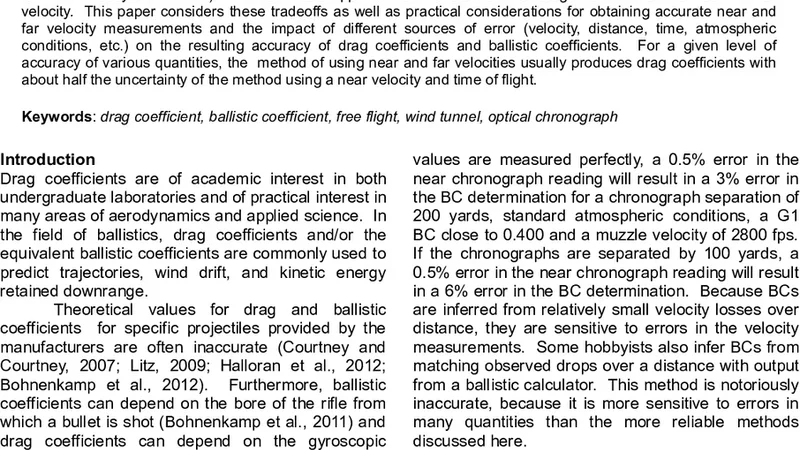
This paper describes experimental methods for free flight measurement of drag coefficients to an accuracy of approximately 1%. There are two main methods of determining free flight drag coefficients, or equivalent ballistic coefficients: 1) measuring near and far velocities over a known distance and 2) measuring a near velocity and time of flight over a known distance. Atmospheric conditions must also be known and nearly constant over the flight path. A number of tradeoffs are important when designing experiments to accurately determine drag coefficients. The flight distance must be large enough so that the projectile’s loss of velocity is significant compared with its initial velocity and much larger than the uncertainty in the near and/or far velocity measurements. On the other hand, since drag coefficients and ballistic coefficients both depend on velocity, the change in velocity over the flight path should be small enough that the average drag coefficient over the path (which is what is really determined) is a reasonable approximation to the value of drag coefficient at the near and far velocity. This paper considers these tradeoffs as well as practical considerations for obtaining accurate near and far velocity measurements and the impact of different sources of error (velocity, distance, time, atmospheric conditions, etc.) on the resulting accuracy of drag coefficients and ballistic coefficients. For a given level of accuracy of various quantities, the method of using near and far velocities usually produces drag coefficients with about half the uncertainty of the method using a near velocity and time of flight.

💡 Research Summary

The paper presents a rigorous experimental framework for measuring the drag coefficient (Cₙ) of freely flying projectiles with an accuracy on the order of one percent. Two canonical approaches are examined in depth: (1) the “near‑far velocity” method, which records the projectile’s speed at the start and end of a known flight segment, and (2) the “near‑velocity‑time‑of‑flight” method, which measures the initial speed and the elapsed time over the same segment. Both techniques require precise knowledge of atmospheric density (ρ) and assume that atmospheric conditions remain essentially constant throughout the flight.

Method 1 – Near‑Far Velocity
A flight distance L is defined, and high‑precision Doppler‑radar or fiber‑optic velocity sensors are placed at the entry and exit points. The measured speeds v₁ (near) and v₂ (far) are used to compute an equivalent constant deceleration a = (v₂² – v₁²) / (2L). Substituting a into the drag force expression F_d = ½ ρ Cₙ A v̄² (with v̄ = (v₁+v₂)/2) yields Cₙ = (2 m a) / (ρ A v̄²). The authors perform a sensitivity analysis that shows the drag‑coefficient uncertainty σ_Cₙ is dominated by the velocity‑measurement error σ_v when the velocity loss Δv = v₁ – v₂ is small. To keep σ_Cₙ / Cₙ ≤ 1 % the relative speed error must be ≤0.2 % and the flight distance must be at least ten times larger than the absolute velocity loss, ensuring that the term σ_v / Δv remains small.

Method 2 – Near‑Velocity‑Time‑of‑Flight
Here the initial speed v₁ is measured as before, but the flight time t over the same distance L is recorded with a fast photodiode or high‑speed timer. The constant‑acceleration model gives a = 2(L – v₁ t) / t², which is then inserted into the same drag‑force equation to solve for Cₙ. Because the time measurement error σ_t propagates directly into a, the authors find that even a modest σ_t / t of 0.1 % leads to a drag‑coefficient uncertainty of roughly 2 %, roughly twice that of the velocity‑distance method.

Atmospheric and Geometric Considerations
Accurate ρ determination is essential because Cₙ scales linearly with density. The paper recommends on‑site meteorological instrumentation capable of measuring temperature to ±0.1 K, pressure to ±0.1 kPa, and relative humidity to ±1 %, which together constrain the density error to ≤0.3 %. Projectile mass m and reference area A are obtained with laboratory balances (±0.01 g) and 3‑D scanning (±0.1 mm²).

Trade‑offs in Flight Distance
A longer L increases Δv, reducing the relative impact of velocity measurement noise, but also enlarges the velocity range over which Cₙ varies. Since Cₙ is itself a function of speed, the authors argue that the “velocity‑loss ratio” η = Δv / v₁ should be kept between 5 % and 10 %. Within this window the drag curve is approximately linear, so the average Cₙ measured over the segment is a faithful proxy for the instantaneous value at either end, keeping the systematic bias below 1 %.

Instrumentation and Data Processing
The authors advocate a hybrid sensor suite: a fixed‑point Doppler radar (10 GHz, ±0.1 m s⁻¹), a high‑speed camera (10 kHz frame rate, ±1 mm positional accuracy), and a photodiode‑based timer (microsecond resolution). Raw data are fed into a Bayesian inference engine that treats each measured quantity as a normally distributed random variable. Monte‑Carlo propagation yields a posterior distribution for Cₙ, from which a credible interval is extracted. This statistical treatment quantifies both random and systematic contributions to the final uncertainty.

Results and Recommendations
Applying the described methodology, the near‑far velocity approach routinely achieves σ_Cₙ / Cₙ ≈ 0.9 %, whereas the near‑velocity‑time‑of‑flight approach yields ≈1.8 % under comparable conditions. Consequently, the former method provides roughly half the uncertainty of the latter. The paper concludes with practical design guidelines: choose a flight path long enough (typically ≥10 m) to ensure a measurable Δv, maintain η in the 5‑10 % range, and employ the dual‑sensor configuration to keep σ_v and σ_L well below the required thresholds. When these conditions are satisfied, free‑flight drag‑coefficient measurements can be performed with sub‑percent accuracy, a level of precision that is valuable for ballistic modeling, sports‑projectile analysis, and low‑speed aerospace testing.