Machine Learning with Operational Costs

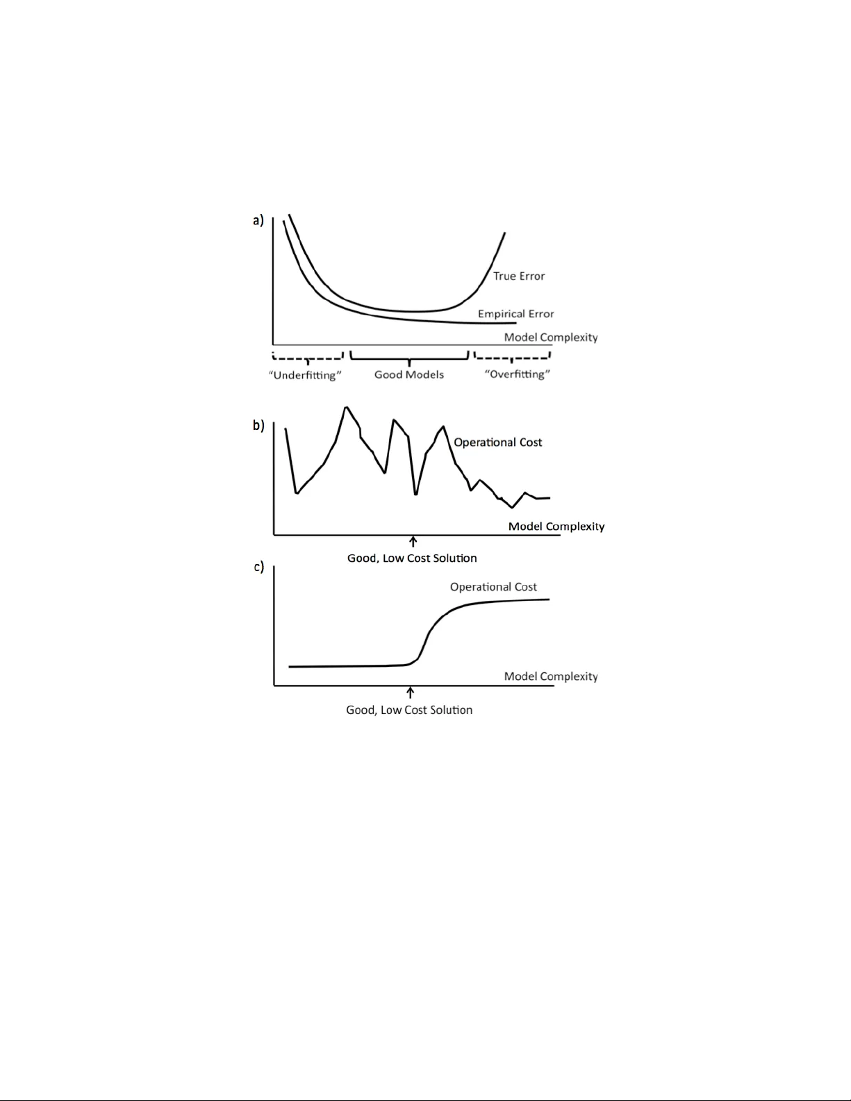
Mac hine Learning with Op erational Costs Theja T ulabandh ula theja@mit.edu Dep artment of Ele ctric al Engine ering and Computer Scienc e Massachusetts Institute of T e chnolo gy Cambridge, MA 02139, USA Cyn thia Rudin rudin@mit.edu MIT Slo an Scho ol of Management and Op er ations R ese ar ch Center Massachusetts Institute of T e chnolo gy Cambridge, MA 02139, USA Abstract This work proposes a wa y to align statistical mo deling with decision making. W e pro vide a metho d that propagates the uncertain ty in predictiv e mo deling to the uncertain ty in op erational cost, where op erational cost is the amount spent b y the practitioner in solving the problem. The metho d allo ws us to explore the range of operational costs asso ciated with the set of reasonable statistical mo dels, so as to pro vide a useful wa y for practitioners to understand uncertain ty . T o do this, the op erational cost is cast as a regularization term in a learning algorithm’s ob jective function, allo wing either an optimistic or p essimistic view of p ossible costs, depending on the regularization parameter. F rom another p erspective, if we hav e prior knowledge ab out the op erational cost, for instance that it should be low, this knowledge can help to restrict the hypothesis space, and can help with generalization. W e pro vide a theoretical generalization b ound for this scenario. W e also sho w that learning with operational costs is related to robust optimization. Keyw ords: statistical learning theory , optimization, cov ering num b ers, decision theory 1. Introduction Mac hine learning algorithms are used to pro duce predictions, and these predictions are often used to make a p olicy or plan of action afterw ards, where there is a cost to implement the p olicy . In this w ork, we would like to understand ho w the uncertain ty in predictiv e mo deling can translate in to the uncertain t y in the cost for implementing the p olicy . This would help us answ er questions like: Q1. “What is a reasonable amoun t to allo cate for this task so we can react b est to whatever nature brings?” Q2. “Can w e produce a reasonable probabilistic model, supp orted b y data, where w e migh t exp ect to pay a sp eciﬁc amount?” Q3. “Can our in tuition ab out ho w muc h it will cost to solve a problem help us pro duce a b etter probabilistic mo del?” The three questions ab ov e cannot be answered b y standard decision theory , where the goal is to pro duce a single p olicy that minimizes expected cost. These questions also cannot be answered b y robust optimization, where the goal is to pro duce a single p olicy that is robust to the uncertain ty in nature. Those paradigms pro duce a single p olicy decision that tak es uncertain ty in to accoun t, c  2012 Theja T ulabandh ula and Cynthia Rudin. and the chosen p olicy might not be a best resp onse p olicy to any realistic situation. In con trast, our goal is to understand the uncertain ty and ho w to react to it, using p olicies that w ould b e b est resp onses to individual situations. There are man y applications in whic h this metho d can be used. F or example, in sc heduling staﬀ for a medical clinic, predictions based on a statistical mo del of the n umber of patients might b e used to understand the p ossible policies and costs for staﬃng. In traﬃc ﬂo w problems, predictions based on a model of the forecasted traﬃc migh t b e useful for determining load balancing policies on the net work and their asso ciated costs. In online adv ertising, predictions based on mo dels for the pa yoﬀ and ad-click rate migh t b e used to understand p olicies for when the ad should b e display ed and the asso ciated rev enue. In order to propagate the uncertain ty in mo deling to the uncertain ty in costs, w e in tro duce what w e call the simultane ous pr o c ess , where w e explore the range of predictiv e models and corresponding p olicy decisions at the same time. T he sim ultaneous pro cess was named to contrast with a more traditional se quential pr o c ess , where ﬁrst, data are input into a statistical algorithm to pro duce a predictiv e mo del, which makes recommendations for the future, and second, the user develops a plan of action and pro jected cost for implementing the p olicy . The sequential pro cess is commonly used in practice, even though there may actually b e a whole class of mo dels that could b e relev an t for the p olicy decision problem. The sequen tial pro cess essentially assumes that the probabilistic mo del is “correct enough” to make a decision that is “close enough.” In the simultaneous pro cess, the mac hine learning algorithm con tains a regularization term enco ding the p olicy and its asso ciated cost, with an adjustable regularization parameter. If there is some uncertain ty about how m uch it will cost to solve the problem, the regularization parameter can b e swept through an interv al to ﬁnd a range of p ossible costs, from optimistic to p essimistic. The metho d then pro duces the most lik ely scenario for eac h v alue of the cost. This wa y , b y looking at the full range of the regularization parameter, we sw eep out costs for all of the reasonable probabilistic mo dels. This range can be used to determine how muc h might b e reasonably allo cated to solv e the problem. Ha ving the full range of costs for reasonable models can directly answ er the question in the ﬁrst paragraph regarding allo cation, “What is a reasonable amount to allo cate for this task so w e can react best to whatever nature brings?” One might choose to allo cate the maximum cost for the set of reasonable predictive mo dels for instance. The second question ab o ve is “Can we pro duce a reasonable probabilistic model, supp orted b y data, where w e migh t exp ect to pa y a sp eciﬁc amount?” This is an important question, since business managers often lik e to kno w if there is some scenario/decision pair that is supp orted b y the data, but for which the op erational cost is lo w (or high); the sim ultaneous pro cess w ould b e able to ﬁnd such scenarios directly . T o do this, we would lo ok at the setting of the regularization parameter that resulted in the desired v alue of the cost, and then lo ok at the solution of the simultaneous form ulation, whic h gives the mo del and its corresp onding p olicy decision. Let us consider the third question ab o ve, which is “Can our intuition ab out how muc h it will cost to solv e a problem help us produce a b etter probabilistic mo del?” The regularization parameter can b e interpreted to regulate the strength of our b elief in the op erational cost. If w e hav e a strong b elief in the cost to solve the problem, and if that belief is correct, this will guide the choice of regularization parameter, and will help with prediction. In many real scenarios, a practitioner or domain exp ert migh t truly hav e a prior b elief on the cost to complete a task. Arguably , a manager ha ving this more grounded t yp e of prior b elief is m uch more natural than, for instance, the manager 2 ha ving a prior b elief on the ` 2 norm of the co eﬃcien ts of a linear mo del, or the n um b er of nonzero co eﬃcien ts in the mo del. Being able to enco de this type of prior b elief on cost could p otentially b e helpful for prediction: as with other types of prior b eliefs, it can help to restrict the hypothesis space and can assist with generalization. In this w ork, w e sho w that the restricted h yp othesis spaces resulting from our method can often b e bounded by an intersection of an an ` q ball with a halfspace - and this is true for many diﬀeren t types of decision problems. W e analyze the complexit y of this t yp e of h yp othesis space with a tec hnique based on Maurey’s Lemma (Barron, 1993; Zhang, 2002) that leads ev entually to a coun ting problem, where w e calculate the n um b er of in teger p oin ts within a p olyhedron in order to obtain a cov ering num b er b ound. The operational cost regularization term can be the optimal v alue of a complicated optimization problem, like a scheduling problem. This means we will need to solv e an optimization problem eac h time w e ev aluate the learning algorithm’s ob jectiv e. How ev er, the practitioner m ust b e able to solv e that problem anyw a y in order to dev elop a plan of action; it is the same problem they need to solv e in the traditional sequential pro cess, or using standard decision theory . Since the decision problem is solved only on data from the presen t, whose labels are not y et kno wn, solving the decision problem may not be diﬃcult, especially if the n umber of unlab eled examples is small. In that case, the method can still scale up to huge historical data sets, since the historical data factors into the training error term but not the new regularization term, and b oth terms can be computed. An example is to compute a schedule for a da y , based on factors of the v arious meetings on the sc hedule that da y . W e can use a very large amoun t of past meeting-length data for the training error term, but then w e use only the small set of p ossible meetings coming up that da y to pass into the sc heduling problem. In that case, both the training error term and the regularization term are able to b e computed, and the ob jective can b e minimized. The sim ultaneous process is a t yp e of decision theory . T o giv e some background, there are t wo types of relev ant decision theories: normativ e (whic h assumes full information, rationality and inﬁnite computational p o wer) and descriptive (mo dels realistic human b eha vior). Normativ e deci- sion theories that address decision making under uncertaint y can b e classiﬁed into those based on ignorance (using no probabilistic information) and those based on risk (using probabilistic informa- tion). The former include maximax, maximin (W ald), minimax regret (Sa v age), criterion of realism (Hurwicz), equally likely (Laplace) approaches. The latter include utility based exp ected v alue and ba yesian approac hes (Sav age). Info-gap, Dempster-Shafer, fuzzy logic, and p ossibilit y theories of- fer non-probabilistic alternativ es to probability in Bay esian/exp ected v alue theories (F renc h, 1986; Hansson, 1994). The sim ultaneous pro cess do es not ﬁt into any of the decision theories listed ab o v e. F or instance, a core idea in the Ba yesian approac h is to c ho ose a single policy that maximizes exp ected utilit y , or minimizes exp ected cost. Our goal is not to ﬁnd a single p olicy that is useful on av erage. In con trast, our goal is to trace out a path of models, their sp eciﬁc (not a v erage) optimal-response policies, and their costs. The p olicy from the Ba yesian approac h may not corresp ond to the b est decision for an y particular single mo del, whereas that is something we w ant in our case. W e trace out this path by c hanging our prior b elief on the op erational cost (that is, by c hanging the strength of our regularization term). In Bay esian decision theory , the prior is o ver p ossible probabilistic mo dels, rather than on p ossible costs as in this pap er. Constructing this prior ov er p ossible probabilistic mo dels can b e challenging, and the prior often ends up b eing chosen arbitrarily , or as a matter of con venience. In contrast, w e assume only an unkno wn probabilit y measure o ver the data, and the data itself deﬁnes the p ossible probabilistic mo dels for which w e compute p olicies. 3 Maximax (optimistic) and maximin (p essimistic) decision approaches con trast with the Ba yesian framew ork and do not assume a distribution on the p ossible probabilistic mo dels. In Section 4 we will discuss how these approaches are related to the simultaneous pro cess. They ov erlap with the sim ultaneous pro cess but not completely . Robust optimization is a maximin approach to decision making, and the sim ultaneous pro cess also diﬀers in principle from robust optimization. In robust optimization, one w ould generally need to allo cate m uch more than is necessary for an y single realistic situation, in order to pro duce a p olicy that is robust to almost all situations. Ho wev er, this is not alw ays true; in fact, we show in this work that in some circumstances, while sweeping through the regularization parameter, one of the results pro duced b y the simultaneous pro cess is the same as the one coming from robust optimization. W e in tro duce the sequen tial and sim ultaneous processes in Section 2. In Section 3, w e giv e sev eral examples of algorithms that incorp orate these op erational costs. In doing so, we pro vide answ ers for the ﬁrst tw o questions Q1 and Q2 ab ov e, with resp ect to sp eciﬁc problems. Our ﬁrst example application is a staﬃng problem at a medical clinic, where the decision problem is to staﬀ a set of stations that patients m ust complete in a certain order. The time required for patien ts to complete eac h station is random and estimated from past data. The second example is a real-estate purc hasing problem, where the p olicy decision is to purchase a subset of av ailable prop erties. The v alues of the prop erties need to b e estimated from comparable sales. The third example is a call cen ter staﬃng problem, where w e need to create a staﬃng p olicy based on historical call arriv al and service time information. A fourth example is the “Machine Learning and T ra veling Repairman Problem” (ML&TRP) where the p olicy decision is a route for a repair crew. As mentioned abov e, there is a large subset of problems that can b e form ulated using the simultaneous pro cess that ha ve a sp ecial prop ert y: they are equiv alent to robust optimization (RO) problems. Section 4 discusses this relationship and pro vides, under sp eciﬁc conditions, the equiv alence of the sim ultaneous process with RO. Robust optimization, when used for decision-making, do es not usually include machine learning, nor an y other type of statistical mo del, so we discuss ho w a statistical model can b e incorp orated within an uncertaint y set for an RO. Sp eciﬁcally , w e discuss how diﬀeren t loss functions from mac hine learning corresp ond to diﬀerent uncertaint y sets. W e also discuss the o verlap b et w een R O and the optimistic and p essimistic versions of the sim ultaneous pro cess. W e consider the implications of the sim ultaneous pro cess on statistical learning theory in Section 5. In particular, we aim to understand ho w op erational costs aﬀect prediction (generalization) abilit y . This helps answer the third question Q3, ab out how intuition ab out op erational cost can help pro duce a b etter probabilistic model. W e sho w ﬁrst that the h yp othesis spaces for most of the applications in Section 3 can b e b ounded in a sp eciﬁc wa y - b y an in tersection of a ball and a halfspace - and this is true regardless of how complicated the constraints of the optimization problem are, and ho w diﬀerent the op erational costs are from each other in the diﬀeren t applications. Second, w e bound the complexit y of this type of h yp othesis space using a tec hnique based on Maurey’s Lemma (Barron, 1993; Zhang, 2002) that leads even tually to a coun ting problem, where w e calculate the num b er of in teger p oin ts within a p olyhedron in order to obtain a generalization b ound. Our results show that it is p ossible to make use of m uch more general structure in estimation problems, compared to the standard (norm-constrained) structures like sparsity and smo othness; further, this additional structure can b eneﬁt generalization abilit y . A shorter version of this work has b een previously published (see T ulabandh ula and Rudin, 2012). 4 2. The Sequen tial and Simultaneous Pro cesses W e hav e a training set of (random) lab eled instances, { ( x i , y i ) } n i =1 , where x i ∈ X , y i ∈ Y that we will use to learn a function f ∗ : X → Y . Commonly in machine learning this is done b y c ho osing f to b e the solution of a minimization problem: f ∗ ∈ argmin f ∈F unc n X i =1 l ( f ( x i ) , y i ) + C 2 R ( f ) ! , (1) for some loss function l : Y × Y → R + , regularizer R : F unc → R , constant C 2 and function class F unc . Here, Y ⊂ R . T ypical loss functions used in machine learning are the 0-1 loss, ramp loss, hinge loss, logistic loss and the exp onen tial loss. F unction class F unc is commonly the class of all linear functionals, where an element f ∈ F unc is of the form β T x , where X ⊂ R p , β ∈ R p . W e ha ve used ‘ unc ’ in the sup erscript for F unc to refer to the w ord “unconstrained,” since it con tains all linear functionals. T ypical regularizers R are the ` 1 and ` 2 norms of β . Note that nonlinearities can b e incorp orated in to F unc b y allowing nonlinear features, so that w e now w ould ha ve f ( x ) = P p j =1 β j h j ( x ), where { h j } j is the set of features, which can b e arbitrary nonlinear functions of x ; for simplicity in notation, w e will equate h j ( x ) = x j and hav e X ⊂ R p . Consider an organization making p olicy decisions. Given a new collection of unlab eled instances { ˜ x i } m i =1 , the organization w an ts to create a p olicy π ∗ that minimizes a certain operational cost OpCost( π , f ∗ , { ˜ x i } i ). Of course, if the organization knew the true lab els for the { ˜ x i } i ’s b eforehand, it w ould c ho ose a policy to optimize the op erational cost based directly on these lab els, and would not need f ∗ . Since the lab els are not kno wn, the op erational costs are calculated using the mo del’s predictions, the f ∗ ( ˜ x i )’s. The diﬀerence b et w een the traditional sequen tial pro cess and the new sim ultaneous pro cess is whether f ∗ is chosen with or without knowledge of the op erational cost. As an example, consider { ˜ x i } i as representing mac hines in a factory w aiting to be repaired, where the ﬁrst feature ˜ x i, 1 is the age of the mac hine, the second feature ˜ x i, 2 is the condition at its last insp ection, etc. The v alue f ∗ ( ˜ x i ) is the predicted probability of failure for ˜ x i . P olicy π ∗ is the order in which the mac hines { ˜ x i } i are repaired, which is chosen based on how lik ely they are to fail, that is, { f ∗ ( ˜ x i ) } i , and on the costs of the v arious t yp es of repairs needed. The traditional sequen tial process pic ks a mo del f ∗ , based on past failure data without the knowledge of op erational cost, and afterwards computes π ∗ based on an optimization problem in volving the { f ∗ ( ˜ x i ) } i ’s and the op erational cost. The new simultaneous process picks f ∗ and π ∗ at the same time, based on optimism or p essimism on the op erational cost of π ∗ . F ormally , the sequential pro cess computes the p olicy according to tw o steps, as follows. Step 1: Create function f ∗ based on { ( x i , y i ) } i according to (1). That is f ∗ ∈ argmin f ∈F unc n X i =1 l ( f ( x i ) , y i ) + C 2 R ( f ) ! . Step 2: Cho ose p olicy π ∗ to minimize the op erational cost, π ∗ ∈ argmin π ∈ Π OpCost( π , f ∗ , { ˜ x i } i ) . The op erational cost OpCost( π , f ∗ , { ˜ x i } i ) is the amount the organization will spend if p olicy π is c hosen in resp onse to the v alues of { f ∗ ( ˜ x i ) } i . 5 T o deﬁne the simultaneous pro cess , w e com bine Steps 1 and 2 of the sequential pro cess. W e can choose an optimistic bias , where w e prefer (all else b eing equal) a mo del providing lo wer costs, or w e can c ho ose a p essimistic bias that prefers higher costs, where the degree of optimism or p essimism is controlled b y a parameter C 1 . in other w ords, the optimistic bias low ers costs when there is uncertain ty , whereas the p essimistic bias raises them. The new steps are as follo ws. Step 1: Cho ose a mo del f ◦ ob eying one of the follo wing: Optimistic Bias: f ◦ ∈ argmin f ∈F unc " n X i =1 l ( f ( x i ) , y i ) + C 2 R ( f ) + C 1 min π ∈ Π OpCost ( π , f , { ˜ x i } i )  (2) P essimistic Bias: f ◦ ∈ argmin f ∈F unc " n X i =1 l ( f ( x i ) , y i ) + C 2 R ( f ) − C 1 min π ∈ Π OpCost ( π , f , { ˜ x i } i )  . (3) Step 2: Compute the p olicy: π ◦ ∈ argmin π ∈ Π OpCost ( π , f ◦ , { ˜ x i } i ) . When C 1 = 0, the simultaneous pro cess becomes the sequential process; the sequential process is a sp ecial case of the sim ultaneous pro cess. The optimization problem in the simultaneous pro cess can b e computationally diﬃcult, par- ticularly if the subproblem to minimize OpCost in volv es discrete optimization. How ever, if the n umber of unlab eled instances is small, or if the p olicy decision can b e brok en into sev eral smaller subproblems, then even if the training set is large, one can solve Step 1 using diﬀeren t t yp es of mathematical programming solv ers, including MINLP solvers (Bonami et al., 2008), Nelder-Mead (Nelder and Mead, 1965) and Alternating Minimization sc hemes (T ulabandh ula et al., 2011). One needs to b e able to solv e instances of that optimization problem in any case for Step 2 of the sequen tial pro cess. The simultaneous process is more intensiv e than the sequen tial pro cess in that it requires rep eated solutions of that optimization problem, rather than a single solution. The regularization term R ( f ) can b e for example, an ` 1 or ` 2 regularization term to encourage a sparse or smo oth solution. As the C 1 co eﬃcien t swings b et ween large v alues for optimistic and p essimistic cases, the algorithm ﬁnds the best solution (having the lo west loss with resp ect to the data) for each p ossible cost. Once the regularization co eﬃcien t is too large, the algorithm will sacriﬁce empirical error in fa vor of low er costs, and will th us obtain solutions that are not reasonable. When that happens, w e know we hav e already mapp ed out the full range of costs for reasonable solutions. This range can b e used for pre-allo cation decisions. By sw eeping ov er a range of C 1 , we obtain a range of costs that we migh t incur. Based on this range, w e can choose to allo cate a reasonable amount of resources so that we can react b est to whatev er nature brings. This helps answ er question Q1 in Section 1. In addition, we can pic k a v alue of C 1 suc h that the resulting op erational cost is a sp eciﬁc amount. In this case, w e chec king whether a probabilistic mo del exists, corresp onding to that cost, that is reasonably supp orted by data. This can answer question Q2 in Section 1. 6 It is p ossible for the set of feasible policies Π to dep end on recommendations { f ( ˜ x 1 ) , ..., f ( ˜ x m ) } , so that Π = Π( f , { ˜ x i } i ) in general. W e will revisit this p ossibility in Section 4. It is also p ossible for the optimization ov er π ∈ Π to b e trivial, or the optimization problem could ha v e a closed form solution. Our notation do es accommo date this, and is more general. One should not view the op erational cost as a utilit y function that needs to b e estimated, as in reinforcemen t learning, where we do not kno w the cost. Here one kno ws precisely what the cost will b e under each p ossible outcome. Unlik e in reinforcemen t learning, w e ha ve a complicated one shot decision problem at hand and hav e training data as w ell as future/unlabeled examples on which the predictive mo del mak es prediction on. The use of unlab eled data { ˜ x i } i has b een explored widely in the mac hine learning literature under semi-supervised, transductive, and unsup ervised learning. In particular, w e p oin t out that the simultaneous process is not a semi-sup ervised learning metho d (see Chap elle et al., 2006), since it do es not use the unlab eled data to pro vide information ab out the underlying distribution. A small unlabeled sample is not v ery useful for semi-sup ervised learning, but could be very useful for constructing a lo w-cost p olicy . The simultaneous pro cess also has a resemblance to transductive learning (see Zh u, 2007), whose goal is to pro duce the output lab els on the set of unlab eled examples; in this case, we pro duce a function (namely the operational cost) applied to those output lab els. The sim ultaneous pro cess, for a ﬁxed choice of C 1 , can also b e considered as a multi-ob jectiv e machine learning metho d, since it inv olves an optimization problem ha ving t wo terms with comp eting goals (see Jin, 2006). 2.1 The Sim ultaneous Pro cess in the Con text of Structural Risk Minimization In the framework of statistical learning theory (e.g., V apnik, 1998; P ollard, 1984; An thon y and Bartlett, 1999; Zhang, 2002), prediction abilit y of a class of models is guaranteed when the class has low “complexit y ,” where complexity is deﬁned via cov ering num b ers, V C (V apnik-Chervonenkis) dimension, Rademac her complexit y , gaussian complexit y , etc. Limiting the complexit y of the h y- p othesis space imp oses a bias, and the classical image asso ciated with the bias-v ariance tradeoﬀ is provided in Figure 1(a). The set of go od mo dels is indicated on the axis of the ﬁgure. Mo dels that are not go od are either o verﬁtted (explaining to o m uch of the v ariance of the data, having a high complexit y), or underﬁtted (having to o strong of a bias and a high empirical error). By understanding complexit y , we can ﬁnd a mo del class where b oth the training error and the com- plexit y are kept lo w. An example of increasingly complex mo del classes is the set of nested classes of polynomials, starting with constants, then linear functions, second order polynomials and so on. In predictive modeling problems, there is often no one righ t statistical mo del when dealing with ﬁnite datasets, in fact there may be a whole class of goo d models. In addition, it is possible that a small change in the c hoice of predictive mo del could lead to a large c hange in the cost required to implemen t the p olicy recommended by the mo del. This o ccurs, for instance, when costs are based on ob jects (e.g., pro ducts) that come in discrete amounts. Figure 1(b) illustrates this possibility , b y sho wing that there may b e a v ariety of costs amongst the class of go o d mo dels. The sim ultaneous pro cess can ﬁnd the range of costs for the set of go od mo dels, which can b e used for allo cation of costs, as discussed in the ﬁrst question Q1 in the introduction. Recall that question Q3 asked if our intuition ab out how m uch it will cost to solv e a problem can help us pro duce a better probabilistic model. Figure 1 can be used to illustrate ho w this question can b e answered. Assume we hav e a strong prior b elief that the op erational cost will not b e ab o ve a certain ﬁxed amount. Accordingly , we will choose only amongst the class of lo w 7 Figure 1: In all three plots, the x-axis represents mo del classes with increasing complexit y . a) Relationship b etw een training error and test error as a function of mo del complexity . b) A p ossible op erational cost as a function of mo del complexit y . c) Another p ossible op erational cost. 8 cost mo dels. This can signiﬁcantly limit the complexit y of the hypothesis space, b ecause the set of lo w-cost go o d mo dels migh t b e m uch smaller than the full space of go o d mo dels. Consider, for example, the cost display ed in Figure 1(c), where only models on the left part of the plot w ould be considered, since they are lo w cost models. Because the hypothesis space is smaller, w e ma y b e able to pro duce a tighter b ound on the complexit y of the hypothesis space, thereby obtaining a b etter prediction guarantee for the sim ultaneous pro cess than for the sequen tial pro cess. In Section 5 we dev elop results of this type. These results indicate that in some cases, the op erational cost can b e an imp ortan t quan tity for generalization. 3. Conceptual Demonstrations W e provide four examples. In the ﬁrst, w e estimate manp o wer requirements for a scheduling task. In the second, we estimate real estate prices for a purc hasing decision. In the third, w e estimate call arriv al rates for a call center staﬃng problem. In the fourth, w e estimate failure probabilities for manholes (access points to an underground electrical grid). The ﬁrst tw o are small scale repro ducible examples, designed to demonstrate new types of constraints due to op erational costs. In the ﬁrst example, the op erational cost subproblem inv olv es scheduling. In the second, it is a knapsack problem, and in the third, it is another m ultidimensional knapsac k v ariant. In the fourth, it is a routing problem. In the ﬁrst, second and fourth examples, the op erational cost leads to a linear constraint, while in the third example, the cost leads to a quadratic constraint. Throughout this section, w e will assume that w e are working with linear functions f of the form β T x so that Π( f , { ˜ x i } i ) can be denoted b y Π( β , { ˜ x i } i ). W e will set R ( f ) to be equal to k β k 2 2 . W e will also use the notation F R to denote the set of linear functions that satisfy an additional prop ert y: F R := { f ∈ F unc : R ( f ) ≤ C ∗ 2 } , where C ∗ 2 is a kno wn constan t greater than zero. W e will use constant C 2 from (1), and also C ∗ 2 from the deﬁnition of F R , to con trol the extent of regularization. C 2 is inv ersely related to C ∗ 2 . W e use b oth versions in terchangeably throughout the pap er. 3.1 Manp o w er Data and Scheduling with Precedence Constraints W e aim to schedule the starting times of medical staﬀ, who work at 6 stations, for instance, ultrasound, X-ray , MRI, CT scan, nuclear imaging, and blo o d lab. Curren t and incoming patients need to go through some of these stations in a particular order. The six stations and the p ossible orders are shown in Figure 2. Each station is denoted b y a line. W ork starts at the c heck-in (at time π 1 ) and ends at the chec k-out (at time π 5 ). The stations are n umbered 6-11, in order to av oid confusion with the times π 1 - π 5 . The clinic has precedence constrain ts, where a station cannot be staﬀed (or w ork with patients) until the preceding stations are lik ely to ﬁnish with their patients. F or instance, the c hec k-out should not start until all the previous stations ﬁnish. Also, as sho wn in Figure 2, station 11 should not start until stations 8 and 9 are complete at time π 4 , and station 9 should not start un til station 7 is complete at time π 3 . Stations 8 and 10 should not start until station 6 is complete. (This is related to a similar problem called planning with pr efer enc e p osed b y F. Malucelli, Politecnico di Milano). The op erational goal is to minimize the total time of the clinic’s operation, from when the c heck-in happens at time π 1 un til the chec k-out happ ens at time π 5 . W e estimate the time it tak es for eac h station to ﬁnish its job with the patien ts based on tw o v ariables: the new load of 9 Figure 2: Staﬃng estimation with bias on scheduling with precedence constraints. patien ts for the day at the station, and the n umber of current patients already presen t. The data are a v ailable as manp ower in the R-pack age b estglm , using “Hour,” “Load” and “Stay” columns. The training error is chosen to b e the least squares loss b et ween the estimated time for stations to ﬁnish their jobs ( β T x i ) and the actual times it to ok to ﬁnish ( y i ). The unlabeled data are the new load and current patien ts present at each station for a giv en p erio d, given as ˜ x 6 , .., ˜ x 11 . Let π denote the 5-dimensional real vector with co ordinates π 1 , ..., π 5 . The op erational cost is the total time π 5 − π 1 . Step 1, with an optimistic bias, can b e written as: min { β : k β k 2 2 ≤ C ∗ 2 } n X i =1 ( y i − β T x i ) 2 + C 1 min π ∈ Π( β, { ˜ x i } i ) ( π 5 − π 1 ) , (4) where the feasible set Π( β , { ˜ x i } i ) is deﬁned by the following constrain ts: π a + β T ˜ x i ≤ π b ; ( a, i, b ) ∈ { (1 , 6 , 2) , (1 , 7 , 3) , (2 , 8 , 4) , (3 , 9 , 4) , (2 , 10 , 5) , (4 , 11 , 5) } π a ≥ 0 for a = 1 , ..., 5 . T o solve (4) giv en v alues of C 1 and C 2 , we used a function-ev aluation-based scheme called Nelder- Mead (Nelder and Mead, 1965) where at ev ery iterate of β , the subproblem for π was solved to optimality (using Gurobi 1 ). C 2 w as c hosen heuristically based on (1) and k ept ﬁxed for the exp erimen t b eforehand. Figure 3 sho ws the operational cost, training loss, and r 2 statistic 2 for v arious v alues of C 1 . F or C 1 v alues b et ween 0 and 0 . 2, the op erational cost v aries substan tially , by ∼ 16%. The r 2 v alues for b oth training and test v ary m uc h less, by ∼ 3.5%, where the b est v alue happ ened to ha ve the largest v alue of C 1 . F or small datasets, there is generally a v ariation b et w een training and test: for this data split, there is a 3.16% diﬀerence in r 2 b et w een training and test for plain least squares, and this is similar across v arious splits of the training and test data. This means that for the scheduling problem, there is a range of reasonable predictiv e mo dels within ab out ∼ 3.5% of each other. 1. Gurobi Optimizer v3.0, Gurobi Optimization, Inc. 2010. 2. If ˆ y i are the predicted lab els and ¯ y is the mean of { y 1 , ..., y n } , then the v alue of the r 2 statistic is deﬁned as 1 − P i ( y i − ˆ y i ) 2 / P i ( y i − ¯ y ) 2 . Thus r 2 is an aﬃne transformation of the sum of squares error. r 2 allo ws training and test accuracy to b e measured on a comparable scale. 10 0 0.05 0.1 0.15 0.2 0 0.5 1 1.5 2 2.5 x 10 4 C 1 Operational Cost 0 0.05 0.1 0.15 0.2 0 2000 4000 6000 8000 C 1 Penalized Training Loss 0 0.05 0.1 0.15 0.2 0 0.2 0.4 0.6 0.8 1 C 1 R ï squared statistic Training Test Figure 3: L eft: Op erational cost vs C 1 . Center: P enalized training loss vs C 1 . R ight: R-squared statistic. C 1 = 0 corresp onds to the baseline, which is the sequen tial form ulation. What w e learn from this, in terms of the three questions in the in tro duction, is that: 1) There is a wide range of p ossible costs within the range of reasonable optimistic mo dels. 2) W e hav e found a reasonable scenario, supp orted b y data, where the cost is 16% low er than in the sequential case. 3) If we hav e a prior b elief that the cost will b e low er, the mo dels that are more accurate are the ones with low er costs, and therefore w e ma y not wan t to designate the full cost suggested b y the sequen tial pro cess. W e can p erhaps designate up to 16% less. Connection to learning theory: In the experiment, we used tradeoﬀ parameter C 1 to provide a soft constraint. Considering instead the corresp onding hard constrain t min π ( π 5 − π 1 ) ≤ α , the total time m ust b e at least the time for an y of the three paths in Figure 2, and th us at least the a verage of them: α ≥ min π ∈ Π { β, { ˜ x i } i } π 5 − π 1 ≥ max { ( ˜ x 6 + ˜ x 10 ) T β , ( ˜ x 6 + ˜ x 8 + ˜ x 11 ) T β , ( ˜ x 7 + ˜ x 9 + ˜ x 11 ) T β } ≥ z T β (5) where z = 1 3 [( ˜ x 6 + ˜ x 10 ) + ( ˜ x 6 + ˜ x 8 + ˜ x 11 ) + ( ˜ x 7 + ˜ x 9 + ˜ x 11 )] . The main result in Section 5, Theorem 6, is a learning theoretic guaran tee in the presence of this kind of arbitrary linear constraint, z T β ≤ α . 3.2 Housing Prices and the Knapsac k Problem A dev elop er will purchase 3 properties amongst the 6 that are currently for sale and in addition, will remo del them. She w ants to maximize the total v alue of the houses she pic ks (the v alue of a prop erty is its purc hase cost plus the ﬁxed remo deling cost). The ﬁxed remo deling costs for the 6 properties are denoted { c i } 6 i =1 . She estimates the purchase cost of eac h property from data regarding historical sales, in this case, from the Boston Housing data set (Bac he and Lic hman, 2013), which has 13 features. Let p olicy π ∈ { 0 , 1 } 6 b e the 6-dimensional binary vector that indicates the prop erties she purchases. Also, x i represen ts the features of prop ert y i in the training data and ˜ x i represen ts the features of a diﬀeren t prop ert y that is currently on sale. The training loss is chosen to b e the 11 sum of squares error b et w een the estimated prices β T x i and the true house prices y i for historical sales. The cost (in this case, total v alue) is the sum of the three prop ert y v alues plus the costs for repair work. A p essimistic bias on total v alue is c hosen to motiv ate a min-max form ulation. T he resulting (mixed-integer) program for Step 1 of the simultaneous pro cess is: min β ∈{ β : β ∈ R 13 , k β k 2 2 ≤ C ∗ 2 } n X i =1 ( y i − β T x i ) 2 + C 1 " max π ∈{ 0 , 1 } 6 6 X i =1 ( β T ˜ x i + c i ) π i sub ject to 6 X i =1 π i ≤ 3 # . (6) Notice that the second term ab o ve is a 1-dimensional { 0 , 1 } knapsac k instance. Since the set of p olicies Π do es not dep end on β , we can rewrite (6) in a cleaner w ay that w as not possible directly with (4): min β max π " n X i =1 ( y i − β T x i ) 2 + C 1 6 X i =1 ( β T ˜ x i + c i ) π i # sub ject to β ∈ { β : β ∈ R 13 , k β k 2 2 ≤ C ∗ 2 } π ∈ ( π : π ∈ { 0 , 1 } 6 , 6 X i =1 π i ≤ 3 ) . (7) T o solve (7) with user-deﬁned parameters C 1 and C 2 , we use fminimax, a v ailable through Matlab’s Optimization to olbox. 3 F or the training and unlab eled set we c hose, there is a c hange in p olicy ab ov e and b elo w C 1 = 0 . 05, where diﬀerent prop erties are purchased. Figure 4 sho ws the op erational cost which is the predicted total v alue of the houses after remo deling, the training loss, and r 2 v alues for a range of C 1 . The training loss and r 2 v alues c hange b y less than ∼ 3.5%, whereas the total v alue c hanges ab out 6 . 5%. W e can again dra w conclusions in terms of the questions in the introduction as follo ws. The p essimistic bias sho ws that ev en if the developer chose the b est resp onse policy to the prices, she might end up with the exp ected total v alue of the purchased prop erties on the order of 6 . 5% less if she is unlucky . Also, w e can now pro duce a realistic mo del where the total v alue is 6 . 5% less. W e can use this mo del to help her understand the uncertain ty inv olved in her in vestmen t. Before mo ving to the next application of the proposed framew ork, w e pro vide a b ound analogous to that of (5). Let us replace the soft constraint represented b y the second term of (6) with a hard constrain t and then obtain a low er b ound: α ≥ max π ∈{ 0 , 1 } 6 , P 6 i =1 π i ≤ 3 6 X i =1 ( β T ˜ x i ) π i ≥ 6 X i =1 ( β T ˜ x i ) π 0 i , (8) where π 0 is some feasible solution of the linear programming relaxation of this problem that also giv es a low er ob jective v alue. F or instance pic king π 0 i = 0 . 5 for i = 1 , . . . , 6 is a v alid low er b ound 3. V ersion 5.1, Matlab R2010b, Mathw orks, Inc. 12 0 0.2 0.4 0.6 0.8 1 65 70 75 80 C 1 Operational Cost 0 0.2 0.4 0.6 0.8 1 55 60 65 70 75 80 C 1 Penalized Training Loss 0 0.2 0.4 0.6 0.8 1 0.5 0.6 0.7 0.8 0.9 1 C 1 R − squared statistic Training Test Figure 4: L eft: Op erational cost (total v alue) vs C 1 . Center: P enalized training loss vs C 1 . R ight: R-squared statistic. C 1 = 0 corresponds to the baseline, which is the sequential formula- tion. giving us a lo oser constraint. The constrain t can b e rewritten: β T 1 2 n X i =1 ˜ x i ! ≤ α. This is again a linear constrain t on the function class parametrized b y β , whic h we can use for the analysis in Section 5. Note that if all six prop erties were b eing purchased by the developer instead of three, the knapsac k problem w ould hav e a trivial solution and the regularization term would be explicit (rather than implicit). 3.3 A Call Cen ter’s W orkload Estimation and Staﬀ Scheduling A call cen ter managemen t wan ts to come up with the per-half-hour sc hedule for the staﬀ for a giv en day b et ween 10am to 10pm. The staﬀ on dut y should b e enough to meet the demand based on call arriv al estimates N ( i ) , i = 1 , ..., 24. The staﬀ required will dep end linearly on the demand per half-hour. The demand p er half-hour in turn will b e computed based on the Erlang C model (Aldor-Noiman et al., 2009) which is also kno wn as the square-ro ot staﬃng rule. This particular mo del relates the demand D ( i ) to the call arriv al rate N ( i ) in the following manner: D ( i ) ∝ N ( i ) + c p N ( i ) where c determines where on the QED (Quality Eﬃciency Driven) curve the cen ter wan ts to op erate on. W e mak e the simplifying assumptions that the service time for eac h customer is constant, and that the co eﬃcien t c is 0. If w e kno w the call arriv al rate N ( i ), we can calculate the staﬃng requirements during each half hour. If we do not know the call arriv al rate, we can estimate it from past data, and make optimistic or p essimistic staﬃng allo cations. There are additional staﬃng constraints as sho wn in Figure 5, namely , there are three sets of emplo yees who w ork at the cen ter suc h that: the ﬁrst set can w ork only from 10am-3pm, the second can w ork from 1:30pm-6:30pm, and the third set works from 5pm-10pm. The op erational cost is the total n um b er of emplo yees hired to work that day (times a constant, which is the amount each p erson is paid). The ob jective of the management is to reduce the num b er of staﬀ on duty but at the same time maintain a certain quality and eﬃciency . 13 Figure 5: The three shifts for the call center. The cells represen t half-hour p erio ds, and there are 24 p erio ds p er w ork da y . W ork starts at 10am and ends at 10pm. The call arriv als are mo deled as a p oisson process (Aldor-Noiman et al., 2009). What previous studies (Bro wn et al., 2001) ha ve disco v ered ab out this estimation problem is that the square ro ot of the call arriv al rate tends to b eha ve as a linear function of several features, including: day of the w eek, time of the day , whether it is a holida y/irregular da y , and whether it is close to the end of the billing cycle. Data for call arriv als and features w ere collected o v er a perio d of 10 mon ths from Mid-F ebruary 2004 to the end of Decem b er 2004 (this is the same dataset as in Aldor-Noiman et al., 2009). After con verting categorical v ariables into binary enco dings (e.g., eac h of the 7 weekda ys in to 6 binary features) the n umber of features is 36, and w e randomly split the data into a training set and test set (2764 instances for training; another 3308 for test). W e now formalize the optimization problem for the simultaneous process. Let p olicy π ∈ Z 3 + b e a size three v ector indicating the num b er of employ ees for eac h of the three shifts. The training loss is the sum of squares error b et ween the estimated square root of the arriv al rate β T x i and the actual square ro ot of the arriv al rate y i := p N ( i ). The cost is prop ortional to the total n umber of emplo y ees signed up to w ork, P i π i . An optimistic bias on cost is chosen, so that the (mixed-in teger) program for Step 1 is: min β : k β k 2 2 ≤ C ∗ 2 n X i =1 ( y i − β T x i ) 2 + C 1 " min π 3 X i =1 π i sub ject to a T i π ≥ ( β T ˜ x i ) 2 for i = 1 , ..., 24 , π ∈ Z 3 + # , (9) 14 0 0.5 1 1.5 2 0 500 1000 1500 C 1 Operational Cost 0 0.5 1 1.5 2 0 2000 4000 6000 8000 C 1 Penalized Training Loss 0 0.5 1 1.5 2 0 0.1 0.2 0.3 0.4 0.5 0.6 C 1 R − squared statistic Training Test Figure 6: L eft: Op erational cost vs C 1 . Center: P enalized training loss vs C 1 . R ight: R-squared statistic. C 1 = 0 corresp onds to the baseline, which is the sequen tial form ulation. where Figure 5 illustrates the matrix A with the shaded cells con taining entry 1 and 0 elsewhere. The notation a i indicates the i th ro w of A : a i ( j ) =  1 if staﬀ j can work in half-hour p eriod i 0 otherwise. T o solv e (9) w e ﬁrst relax the ` 2 -norm constraint on β by adding another term to the function ev aluation, namely C 2 k β k 2 2 . This, w ay we can use a function-ev aluation based scheme that works for unconstrained optimization problems. As in the manp ow er sc heduling example, we used an implemen tation of the Nelder-Mead algorithm, where at each step, Gurobi w as used to solv e the mixed-in teger subproblem for ﬁnding the p olicy . Figure 6 sho ws the op erational cost, the training loss, and r 2 v alues for a range of C 1 . The training loss and r 2 v alues c hange only ∼ 1.6% and ∼ 3.9% resp ectiv ely , whereas the operational cost c hanges ab out 9.2%. Similar to the previous t w o examples, w e can again dra w conclusions in terms of the questions in Section 1 as follows. The optimistic bias sho ws that the managemen t might incur operational costs on the order of 9% less if they are luc ky . F urther, the sim ultaneous pro cess pro duces a reasonable mo del where costs are ab out 9% less. If the managemen t team b eliev es they will be reasonably lucky , they can justify designating substantially less than the amoun t suggested b y the traditional sequential pro cess. Let us no w inv estigate the structure of the op erational cost regularization term w e ha ve in (9). F or conv enience, let us stack the quantities ( β T ˜ x i ) 2 as a v ector b ∈ R 24 . Also let b oldface sym b ol 1 represen t a vector of all ones. If we replace the soft constraint represented by the second term with a hard constraint ha ving an upp er b ound α , we get: α ≥ min π ∈ Z 3 + ; Aπ ≥ b 3 X i =1 1 T π ( † ) ≥ min π ∈ R 3 + ; Aπ ≥ b 3 X i =1 1 T π ( ‡ ) = max w ∈ R 24 + ; A T w ≤ 1 24 X i =1 w i ( β T ˜ x i ) 2 ( ∗ ) ≥ 24 X i =1 1 10 ( β T ˜ x i ) 2 . Here α is related to the choice of C 1 and is ﬁxed. ( † ) represen ts an LP relaxation of the in teger program with π now b elonging to the p ositiv e orthant rather than the cartesian pro duct of set of p ositiv e in tegers. ( ‡ ) is due to LP strong dualit y and ( ∗ ) is by c ho osing an appropriate feasible dual 15 v ariable. Sp eciﬁcally , w e pick w i = 1 10 for i = 1 , . . . , 24, whic h is feasible b ecause staﬀ cannot w ork more than 10 half hour shifts (or 5 hours). With the three inequalities, we now hav e a constraint on β of the form: 24 X i =1 ( β T ˜ x i ) 2 ≤ 10 α. This is a quadratic form in β and giv es an ellipsoidal feasible set. W e already had a simple ellipsoidal feasibilit y constraint while deﬁning the minimization problem of (9) of the form k β k 2 2 ≤ C ∗ 2 . Th us, w e can see that our eﬀectiv e h yp othesis set (the set of linear functionals satisfying these constraints) has becom e smaller. This in turn aﬀects generalization. W e are in vestigating generalization bounds for this t yp e of hypothesis set in separate ongoing w ork. 3.4 The Mac hine Learning and T rav eling Repairman Problem (ML&TRP) (T ulabandh ula et al., 2011) Recen tly , pow er companies hav e b een in vesting in in telligen t “proactiv e” main tenance for the pow er grid, in order to enhance public safety and reliabilit y of electrical service. F or instance, New Y ork Cit y has implemented new insp ection and repair programs for manholes, where a manhole is an access p oin t to the underground electrical system. Electrical grids can b e extremely large (there are on the order of 23,000-53,000 manholes in each borough of NYC), and parts of the underground distribution netw ork in many cities can b e as old as 130 years, dating from the time of Thomas Edison. Because of the diﬃculties in collecting and analyzing historical electrical grid data, electrical grid repair and maintenance has been p erformed reactiv ely (ﬁx it only when it breaks), un til recently (Urbina, 2004). These new proactiv e maintenance programs op en the do or for machine learning to assist with smart grid maintenance. Mac hine learning mo dels ha v e started to b e used for proactiv e maintenance in NYC, where sup ervised ranking algorithms are used to rank the manholes in order of predicted susceptibility to failure (ﬁres, explosions, smok e) so that the most vulnerable manholes can b e prioritized (Rudin et al., 2010, 2012, 2011). The mac hine learning algorithms mak e reasonably accurate predictions of manhole vulnerability; how ever, they do not (nor w ould they , using any other prediction-only tec hnique) take the cost of repairs into account when making the ranked lists. They do not know that it is unreasonable, for example, if a repair crew has to trav el across the city and bac k again for eac h manhole insp ection, losing imp ortan t time in the pro cess. The p o wer company m ust solv e an optimization problem to determine the b est repair route, based on the machine learning mo del’s output. W e migh t wish to ﬁnd a p olicy that is not only supp orted by the historical p o w er grid data (that ranks more vulnerable manholes ab o v e less vulnerable ones), but also w ould give a b etter route for the repair crew. An algorithm that could ﬁnd suc h a route would lead to an improv ement in repair operations on NYC’s p o wer grid, other p o wer grids across the w orld, and improv emen ts in many diﬀeren t kinds of routing op erations (deliv ery truc ks, trains, airplanes). The sim ultaneous pro cess could be used to solve this problem, where the op erational cost is the price to route the repair crew along a graph, and the probabilities of failure at each node in the graph m ust be estimated. W e call this the “the machine learning and tra veling repairman problem” (ML&TRP) and in our ongoing work (T ulabandhula et al., 2011) , we ha ve dev elop ed sev eral formulations for the ML&TRP . W e demonstrated, using manholes from the Bronx region of NYC, that it is possible to obtain a m uch more practical route using the ML&TRP , by taking the cost of the route optimistically in to accoun t in the machine learning mo del. W e sho wed also 16 that from the routing problem, w e can obtain a linear constraint on the hypothesis space, in order to apply the generalization analysis of Section 5 (and in order to address question Q3 of Section 1). 4. Connections to Robust Optimization The goal of robust optimization (R O) is to provide the best p ossible p olicy that is acceptable under a wide range of situations. 4 This is diﬀerent from the sim ultaneous process, which aims to ﬁnd the b est p olicies and costs for sp eciﬁc situations. Note that it is not alw ays desirable to hav e a p olicy that is robust to a wide range of situations; this is a question of whether to resp ond to ev ery situation sim ultaneously or whether to understand the single worst situation that could reasonably o ccur (whic h is what the p essimistic simultaneous form ulation handles). In general, robust optimization can b e ov erly p essimistic, requiring us to allo cate enough to handle all reasonable situations; it can b e substan tially more p essimistic than the p essimistic sim ultaneous pro cess. In robust optimization, if there are several real-v alued parameters inv olved in the optimization problem, w e migh t declare a reasonable range, called the “uncertain ty set,” for eac h parameter ( e.g. a 1 ∈ [9 , 10], a 2 ∈ [1 , 2]). Using techniques of R O, w e would minimize the largest possible operational cost that could arise from parameter settings in these ranges. Estimation is not usually in volv e d in the study of robust optimization (with some exceptions, see Xu et al., 2009, who consider supp ort v ector mac hines). On the other hand, one could choose the uncertain t y set according to a statistical mo del, which is ho w we will build a connection to R O. Here, w e c ho ose the uncertaint y set to b e the class of mo dels that ﬁt the data to within  , according to some ﬁtting criteria. The ma jor goals of the ﬁeld of R O include algorithms, geometry , and tractability in ﬁnding the b est p olicy , whereas our work is not concerned with ﬁnding a robust p olicy , but w e are concerned with estimation, taking the policy in to account. T ractabilit y for us is not alw ays a main concern as w e need to be able to solv e the optimization problem, ev en to use the sequen tial process. Using ev en a small optimization problem as the op erational cost might hav e a large impact on the mo del and decision. If the unlab eled set is not to o large, or if the p olicy optimization problem can b e broken in to smaller subproblems, there is no problem with tractability . An example where the policy optimization migh t b e brok en in to smaller subproblems is when the policy inv olv es routing several diﬀeren t vehicles, where each v ehicle must visit part of the unlab eled set; in that case there is a small subproblem for eac h vehicle. On the other hand, even though the goals of the simultaneous pro cess and R O are entirely diﬀerent, there is a strong connection with resp ect to the form ulations for the simultaneous pro cess and RO, and a class of problems for which they are equiv alent. W e will explore this connection in this section. There are other metho ds that consider uncertaint y in optimization, though not via the lens of estimation and learning. In the simplest case, one can p erform b oth lo cal and global sensitivity analysis for linear programs to ascertain uncertaint y in the optimal solution and ob jectiv e, but these tec hniques generally only handle simple forms of uncertaint y (V anderb ei, 2008). Our w ork is also related to stochastic programming, where the goal is to ﬁnd a p olicy that is robust to almost all of the p ossible circumstances (rather than all of them), where there are random v ariables go verning the parameters of the problem, with kno wn distributions (Birge and Louveaux, 1997). Again, our goal is not to ﬁnd a p olicy that is necessarily robust to (almost all of ) the worst cases, 4. h ttp://en.wikip edia.org/wiki/Robust optimization 17 and estimation is again not the primary concern for sto c hastic programming, rather it is how to tak e kno wn randomness into accoun t when determining the p olicy . 4.1 Equiv alence Bet ween RO and the Simultaneous Process in Some Cases In this subsection we will formally introduce R O. In order to connect RO to estimation, w e will deﬁne the uncertain t y set for R O, denoted F g ood , to b e mo dels for whic h the a verage loss on the sample is within  of the low est p ossible. Then we will presen t the equiv alence relationship b etw een R O and the simultaneous pro cess, using a minimax theorem. In Section 2, w e had in tro duced the notation { ( x i , y i ) } i and { ˜ x i } i for lab eled and unlab eled data resp ectively . W e had also in tro duced the class F unc in which we were searching for a function f ∗ b y minimizing an ob jective of the form (1). The uncertain ty set F g ood will turn out to be a subset of F unc that dep ends on { ( x i , y i ) } i and f ∗ but not on { ˜ x i } i . W e start with plain (non-robust) optimization, using a general v ersion of the v anilla sequen tial pro cess. Let f denote an element of the set F g ood , where f is pre-determined, kno wn and ﬁxed. Let the optimization problem for the p olicy decision π b e deﬁned by: min π ∈ Π( f ; { ˜ x } i ) OpCost( π , f ; { ˜ x i } ) , (Base pr oblem) (10) where Π( f ; { ˜ x i } ) is the feasible set for the optimization problem. Note that this is a more general v ersion of the sequential pro cess than in Section 2, since w e hav e allow ed the constrain t set Π to b e a function of b oth f and { ˜ x i } i , whereas in (2) and (3), only the ob jectiv e and not the constraint set can dep end on f and { ˜ x i } i . Allowing this more general v ersion of Π will allo w us to relate (10) to RO more clearly , and will help us to sp ecify the additional assumptions we need in order to show the equiv alence relationship. Sp eciﬁcally , in Section 2, OpCost depends on ( f , { ˜ x i } i ) but not Π; whereas in RO, generally Π dep ends on ( f , { ˜ x i } i ) but not OpCost. The fact that OpCost do es not need to dep end on f and { ˜ x i } i is not a serious issue, since we can generally remov e their dep endence through auxiliary v ariables. F or instance, if the problem is a minimization of the form (10), we can use an auxiliary v ariable, say t , to obtain an equiv alent problem: min π ,t t (Base pr oblem r eformulate d) suc h that π ∈ Π( f ; { ˜ x i } ) OpCost( π , f ; { ˜ x i } ) ≤ t where the dep endence on ( f , { ˜ x i } i ) is present only in the (new) feasible set. Since w e had assumed f to b e ﬁxed, this is a deterministic optimization problem (conv ex, mixed-in teger, nonlinear, etc.). No w, consider the case when f is not kno wn exactly but only kno wn to lie in the uncertain ty set F g ood . The robust counterpart to (10) can then b e written as: min π ∈ ∩ g ∈F good Π( g ; { ˜ x } i ) max f ∈F good OpCost( π , f ; { ˜ x i } ) (R obust c ounterp art) (11) where we obtain a “robustly feasible solution” that is guaran teed to remain feasible for all v alues of f ∈ F g ood . In general, (11) is m uc h harder to solve than (10) and is a topic of muc h in terest in the robust optimization comm unity . As we discussed earlier, there is no fo cus in (11) on estimation, but it is p ossible to embed an estimation problem within the description of the set F g ood , whic h we no w deﬁne formally . 18 In Section 3, F R (a subset of F unc ) w as deﬁned as the set of linear functionals with the property that R ( f ) ≤ C ∗ 2 . That is, F R = { f : f ∈ F unc , R ( f ) ≤ C ∗ 2 } . W e deﬁne F g ood as a subset of F R b y adding an additional prop ert y: F g ood = ( f : f ∈ F R , n X i =1 l ( f ( x i ) , y i ) ≤ n X i =1 l ( f ∗ ( x i ) , y i ) +  ) , (12) for some ﬁxed p ositiv e real  . In (12), again f ∗ is a solution that minimizes the ob jective in (1) o ver F unc . The right hand side of the inequalit y in (12) is thus constant, and we will henceforth denote it with a single quan tit y C ∗ 1 . Substituting this deﬁnition of F g ood in (11), and further making an imp ortan t assumption (denoted A1 ) that Π is not a function of ( f , { ˜ x i } i ), w e get the following optimization problem: min π ∈ Π max { f ∈F R : P n i =1 l ( f ( x i ) ,y i ) ≤ C ∗ 1 } h OpCost ( π , f , { ˜ x i } i ) i (R obust c ounterp art with assumptions) (13) where C ∗ 1 no w con trols the amount of the uncertaint y via the set F g ood . Before w e state the equiv alence relationship, w e restate the formulations for optimistic and p essimistic biases on op erational cost in the sim ultaneous pro cess from (2) and (3): min f ∈F unc " n X i =1 l ( f ( x i ) , y i ) + C 2 R ( f ) + C 1 min π ∈ Π OpCost ( π , f , { ˜ x i } i ) # (Simultane ous optimistic) min f ∈F unc " n X i =1 l ( f ( x i ) , y i ) + C 2 R ( f ) − C 1 min π ∈ Π OpCost ( π , f , { ˜ x i } i ) # (Simultane ous p essimistic) (14) Apart from the assumption A1 on the decision set Π that we made in (13), w e will also assume that F g ood deﬁned in (12) is con v ex; this will b e assumption A2 . If we also assume that the ob jective OpCost satisﬁes some nice prop erties ( A3 ), and that uncertaint y is characterized via the set F g ood , then w e can sho w that the t wo problems, namely (14) and (13), are equiv alen t. Let ⇔ denote equiv alence b et ween tw o problems, meaning that a solution to one side translates in to the solution of the other side for some parameter v alues ( C 1 , C ∗ 1 , C 2 , C ∗ 2 ). Prop osition 1 L et Π( f ; { ˜ x i } i ) = Π b e c omp act, c onvex, and indep endent of p ar ameters f and { ˜ x i } i (assumption A1 ). L et { f ∈ F R : P n i =1 l ( f ( x i ) , y i ) ≤ C ∗ 1 } b e c onvex (assumption A2 ). L et the c ost (to b e minimize d) OpCost( π , f , { ˜ x i } i ) b e c onc ave c ontinuous in f and c onvex c ontinuous in π (assumption A3 ). Then, the r obust optimization pr oblem (13) is e quivalent to the p essimistic bias optimization pr oblem (14). That is, min π ∈ Π max { f ∈F R : P n i =1 l ( f ( x i ) ,y i ) ≤ C ∗ 1 } h OpCost( π , f , { ˜ x i } i ) i ⇔ min f ∈F unc " n X i =1 l ( f ( x i ) , y i ) + C 2 R ( f ) − C 1 min π ∈ Π OpCost ( π , f , { ˜ x i } i ) # . 19 Remark 2 That the e quivalenc e applies to line ar pr o gr ams (LPs) is cle ar b e c ause the obje ctive is line ar and the fe asible set is gener al ly a p olyhe dr on, and is thus c onvex. F or inte ger pr o gr ams, the obje ctive OpCost satisﬁes c ontinuity, but the fe asible set is typic al ly not c onvex, and henc e, the r esult do es not gener al ly apply to inte ger pr o gr ams. In other wor ds, the r e quir ement that the c onstr aint set Π b e c onvex excludes inte ger pr o gr ams. T o prov e Prop osition 1, we restate a w ell-kno wn generalization of von Neumann’s minimax theorem and some related deﬁnitions. Deﬁnition 3 A line ar top olo gic al sp ac e (also c al le d a top olo gic al ve ctor sp ac e) is a ve ctor sp ac e over a top olo gic al ﬁeld (typic al ly, the r e al numb ers with their standar d top olo gy) with a top olo gy such that ve ctor addition and sc alar multiplic ation ar e c ontinuous functions. F or example, any norme d ve ctor sp ac e is a line ar top olo gic al sp ac e. A function h is upp er semic ontinuous at a p oint p 0 if for every  > 0 ther e exists a neighb orho o d U of p 0 such that h ( p ) ≤ h ( p 0 ) +  for al l p ∈ U . A function h deﬁne d over a c onvex set is quasi-c onc ave if for al l p, q and λ ∈ [0 , 1] we have h ( λp + (1 − λ ) q ) ≥ min( h ( p ) , h ( q )) . Similar deﬁnitions fol low for lower semic ontinuity and quasi-c onvexity. Theorem 4 (Sion ’s minimax the or em Sion, 1958) L et Π b e a c omp act c onvex subset of a line ar top olo gic al sp ac e and Ξ b e a c onvex subset of a line ar top olo gic al sp ac e. L et G ( π , ξ ) b e a r e al function on Π × Ξ such that (i) G ( π , · ) is upp er semic ontinuous and quasi-c onc ave on Ξ for e ach π ∈ Π ; (ii) G ( · , ξ ) is lower semic ontinuous and quasi-c onvex on Π for e ach ξ ∈ Ξ . Then min π ∈ Π sup ξ ∈ Ξ G ( π , ξ ) = sup ξ ∈ Ξ min π ∈ Π G ( π , ξ ) W e can now proceed to the pro of of Prop osition (1). Pro of (Of Pr op osition 1) W e start from the left hand side of the equiv alence we w ant to prov e: min π ∈ Π max { f ∈F R : P n i =1 l ( f ( x i ) ,y i ) ≤ C ∗ 1 } h OpCost( π , f , { ˜ x i } i ) i ( a ) ⇔ max { f ∈F R : P n i =1 l ( f ( x i ) ,y i ) ≤ C ∗ 1 } min π ∈ Π h OpCost( π , f , { ˜ x i } i ) i ( b ) ⇔ max f ∈F unc h − 1 C 1  n X i =1 l ( f ( x i ) , y i ) − C ∗ 1  − C 2 C 1  R ( f ) − C ∗ 2  + min π ∈ Π OpCost( π , f , { ˜ x i } i ) i ( c ) ⇔ min f ∈F unc " n X i =1 l ( f ( x i ) , y i ) + C 2 R ( f ) − C 1 min π ∈ Π OpCost ( π , f , { ˜ x i } i ) # . whic h is the right hand side of the logical equiv alence in the statemen t of the theorem. In step ( a ) w e applied Sion’s minimax theorem (Theorem 4) whic h is satisﬁed b ecause of the assumptions we 20 made. In step ( b ), w e pic ked Lagrange co eﬃcien ts, namely 1 C 1 and C 2 C 1 , b oth of which are p ositiv e. In particular, C ∗ 1 and C 1 as w ell as C ∗ 2 and C 2 are related b y the Lagrange relaxation equiv a- lence (strong duality). In ( c ), w e multiplied the ob jective with C 1 throughout, pulled the negative sign in front, and remov ed the constan t terms C ∗ 1 and C 2 C ∗ 2 and used the following observ ation: max a − g ( a ) = − min a g ( a ); and ﬁnally , remo ved the negativ e sign in fron t as this do es not aﬀect equiv alence. The equiv alence relationship of Proposition 1 sho ws that there is a problem class in which each instance can b e view ed either as a R O problem or an estimation problem with an op erational cost bias. W e can use ideas from RO to mak e the simultaneous pro cess more general. Before doing so, w e will characterize F g ood for several sp eciﬁc loss functions. 4.2 Creating Uncertain ty Sets for RO Using Loss F unctions from Machine Learning Let us for simplicity sp ecialize our loss function to the least squares loss. Let X b e an n × p matrix with eac h training instance x i forming the i th ro w. Also let Y b e the n -dimensional v ector of all the lab els y i . Then the loss term of (1) can b e written as: n X i =1 ( y i − f ( x i )) 2 = n X i =1 ( y i − β T x i ) 2 = k Y − X β k 2 2 . Let β ∗ b e a parameter corresp onding to f ∗ in (1). Then the deﬁnition of F g ood in terms of the least squares loss is: F g ood = { f : f ∈ F R , k Y − X β k 2 2 ≤ k Y − X β ∗ k 2 2 +  } = { f : f ∈ F R , k Y − X β k 2 2 ≤ C ∗ 1 } . Since eac h f ∈ F g ood corresp onds to at least one β , the optimization of (1) can be p erformed with resp ect to β . In particular, the constraint k Y − X β k ≤ C ∗ 1 is an ellipsoid constraint on β . F or the purp oses of the robust counterpart in (11), we can thus say that the uncertain t y is of the ellipsoidal form. In fact, ellipsoidal constraints on uncertain parameters are widely used in robust optimization, esp ecially b ecause the resulting optimization problems often remain tractable. Bo x constrain ts are also a p opular wa y of incorp orating uncertaint y in to robust optimization. F or b o x constraints, the uncertain ty o ver the p -dimensional parameter vector β = [ β 1 , ..., β p ] T is written for i = 1 , ..., p as LB i ≤ β i ≤ U B i , where { LB i } i and { U B i } i are real-v alued upp er and lo wer b ounds that together deﬁne the b o x in terv als. Our main point in this subsection is that one can p oten tially derive a very wide range of uncertain ty sets for robust optimization using diﬀerent loss functions from mac hine learning. Bo x constrain ts and ellipsoidal constraints are t wo simple t yp es of constrain ts that could p oten tially b e the set F g ood , whic h arise from t wo diﬀeren t loss functions, as w e ha ve shown. The least squares loss leads to ellipsoidal constraints on the uncertain ty set, but it is unclear what the structure w ould b e for uncertaint y sets arising from the 0-1 loss, ramp loss, hinge loss, logistic loss and exp onen tial loss among others. F urther, it is p ossible to create a loss function for ﬁtting data to a probabilistic mo del using the metho d of maximum lik eliho o d; uncertaint y sets for maximum lik eliho o d could th us b e established. T able 4.2 shows several diﬀerent p opular loss functions and the uncertaint y sets they might lead to. Many of these new uncertaint y sets do not alwa ys giv e tractable mathematical programs, which could explain wh y they are not commonly considered in the optimization literature. 21 Loss function Uncertain ty set description least squares k Y − X β k 2 2 ≤ k Y − X β ∗ k 2 2 +  (ellipsoid) 0-1 loss 1 [ f ( x i ) 6 = y i ] ≤ 1 [ f ∗ ( x i ) 6 = y i ] +  logistic loss P n i =1 log(1 + e − y i f ( x i ) ) ≤ P n i =1 log(1 + e − y i f ∗ ( x i ) ) +  exp onen tial loss P n i =1 e − y i f ( x i ) ≤ P n i =1 e − y i f ∗ ( x i ) +  ramp loss P n i =1 min(1 , max(0 , 1 − y i f ( x i ))) ≤ P n i =1 min(1 , max(0 , 1 − y i f ∗ ( x i ))) +  hinge loss P n i =1 max(0 , 1 − y i f ( x i )) ≤ P n i =1 max(0 , 1 − y i f ∗ ( x i )) +  T able 1: T able sho wing a summary of diﬀerent p ossible uncertaint y set descriptions that are based on ML loss functions. The sequen tial pro cess for RO. If w e design the uncertain ty sets as describ ed ab o v e, with resp ect to a machine learning loss function, the sequential pro cess describ ed in Section 2 can b e used with robust optimization. This pro ceeds in three steps: 1. use a learning algorithm on the training data to get f ∗ , 2. establish an uncertaint y set based on the loss function and f ∗ , for example, ellipsoidal con- strain ts arising from the least squares loss (or one could use any of the new uncertaint y sets discussed in the previous paragraph), 3. use sp ecialized optimization techniques to solve for the b est p olicy , with resp ect to the un- certain ty set. W e note that the uncertaint y sets created by the 0-1 loss and ramp loss for instance, are non-con vex, consequen tly assumption ( A2 ) and Prop osition 1 do not hold for robust optimization problems that use these sets. 4.3 The Ov erlap Betw een The Simultaneous Pro cess and RO On the other end of the sp ectrum from robust optimization, one can think of “optimistic” opti- mization where we are seeking the b est v alue of the ob jective in the best possible situation (as opp ose to the w orst possible situation in R O). F or optimistic optimization, more uncertaint y is fa vorable, and we ﬁnd the b est p olicy for the b est p ossible situation. This could be useful in man y real applications where one not only wan ts to kno w the w orst-case conserv ative p olicy but also the b est case risk-taking p olicy . A t ypical form ulation, following (11) can b e written as: min π ∈ ∪ g ∈F good Π( g ; { ˜ x } i ) min f ∈F good OpCost( π , f ; { ˜ x i } ) . ( Optimistic optimization ) In optimistic optimization, we view op erational cost optimistically (min f ∈F good OpCost) whereas in the robust optimization counterpart (11), we view op erational cost conserv atively (max f ∈F good OpCost). The p olicy π ∗ is feasible in more situations in R O (min π ∈∩ g ∈F good Π ) since it m ust b e feasible with resp ect to each g ∈ F g ood , whereas the OpCost is lo wer in optimistic optimization (min π ∈∪ g ∈F good Π ) since it need only b e feasible with respect to at least one of the g ’s. Optimistic optimization has not 22 Figure 7: Set based description of the prop osed framew ork (top circle) and its relation to robust (righ t circle) and optimistic (left circle) optimizations. The regions of intersection are where the conditions on the ob jective OpCost and the feasible set Π are satisﬁed. b een heavily studied, possibly b ecause a (min-min) formulation is relativ ely easier to solv e than its (min-max) robust counterpart, and so is less computationally interesting. Also, one generally plans for the w orst cas e more often than for the b est case, particularly when no estimation is in volv ed. In the case where estimation is in volv ed, both optimistic and robust optimization could p oten tially b e useful to a practitioner. Both optimistic optimization and robust optimization, considered with resp ect to uncertaint y sets F g ood , hav e non-trivial ov erlap with the sim ultaneous pro cess. In particular, we show ed in Prop osition 1 that p essimistic bias on op erational cost is equiv alen t to robust optimization under sp eciﬁc conditions on OpCost and Π. Using an analogous proof, one can show that optimistic bias on op erational cost is equiv alent to optimistic optimization under the same set of conditions. Both robust and optimistic optimization and the simultaneous process encompass large classes of problems, some of whic h ov erlap. Figure 7 represents the ov erlap b et w een the three classes of problems. There is a class of problems that fall in to the simultaneous pro cess, but are not equiv alent to robust or optimistic optimization problems. These are problems where w e use operational cost to assist with estimation, as in the call center example and ML&TRP discussed in Section 3. T ypically problems in this class hav e Π = Π( f ; { ˜ x i } i ). This class includes problems where the bias can b e either optimistic or p essimistic, and for whic h F g ood has a complicated structure, beyond ellipsoidal or b o x constraints. There are also problems contained in either robust optimization or optimistic optimization alone and do not belong to the sim ultaneous pro cess. Typically , again, this is when Π dep ends on f . Note that the housing problem presented in Section 3 lies within the intersection of optimistic optimization and the simultaneous process; this can b e deduced from (7). In Section 5, we will provide statistical guarantees for the sim ultaneous pro cess. These are very diﬀeren t from the style of probabilistic guaran tees in the robust optimization literature. There are some “sample complexit y” b ounds in the RO literature of the follo wing form: how man y observ ations of uncertain data are required (and applied as simultaneous constraints) to main tain robustness of the solution with high probability? There is an unfortunate o verlap in terminology; these are totally diﬀeren t problems to the sample complexit y b ounds in statistical learning theory . F rom the learning theory p ersp ectiv e, we ask: ho w many training instances does it take to come 23 Figure 8: Left: h yp othesis space for in tersection of go o d models (circular, to represen t ` q ball) with low cost models (models below cost threshold, one side of wiggly curv e). Right: relaxation to in tersection of a half space with an ` q ball. up with a mo del β that we reasonably know to b e go od? W e will answer that question for a v ery general class of estimation problems. 5. Generalization Bound with New Linear Constrain ts In this section, we give statistical learning theoretic results for the sim ultaneous process that inv olve coun ting integer points in con vex bo dies. Generalization bounds are probabilistic guaran tees, that often depend on some measure of the complexit y of the h yp othesis space. Limiting the complexit y of the h yp othesis space equates to a b etter b ound. In this section, we consider the complexit y of hypothesis spaces that results from an operational cost bias. This enables us to answer in a quan titative manner, question Q3 in the introduction: “Can our in tuition ab out ho w m uch it will cost to solv e a problem help us pro duce a b etter probabilistic mo del?” Generalization bounds ha ve b een well established for norm-b ase d constraints on the hypothesis space, but the emphasis has b een more on qualitativ e dep endence (e.g., using big-O notation) and the constants are not emphasized. On the other hand, for a practitioner, every prior b elief should reduce the n um b er of examples they need to collect, as these examples ma y each b e exp ensiv e to obtain; th us constants within the bounds, and even their approximate v alues, b ecome imp ortan t (Bousquet, 2003). W e thus pro vide b ounds on the co vering n umber for new types of hypothesis spaces, emphasizing the role of constants. T o establish the bound, it is suﬃcien t to pro vide an upp er b ound on the co vering num b er. There are many existing generic generalization b ounds in the literature (e.g., Bartlett and Mendelson, 2002), which combined with our b ound, will yield a speciﬁc generalization bound for mac hine learning with op erational costs, as we will construct in Theorem 10. In Section 3, w e sho wed that a bias on the op erational cost can sometimes b e transformed in to linear constraints on model parameter β (see equations (5) and (8)). There is a broad class of other problems for which this is true, for example, for applications related to those presented in Section 3. Because we are able to obtain linear constrain ts for suc h a broad class of problems, w e will analyze the case of linear constrain ts here. The h yp othesis w e consider is thus the intersection of an ` q ball and a halfspace. This is illustrated in Figure 8. The plan for the rest of the section is as follows. W e will introduce the quantities on which our main result in this section dep ends. Then, we will state the main result (Theorem 6). F ollowing 24 that, w e will build up to a generalization bound (Theorem 10) that incorp orates Theorem 6. After that will b e the pro of of Theorem 6. Deﬁnition 5 (Covering Numb er, Kolmo gor ov and Tikhomir ov, 1959) L et A ⊆ Γ b e an arbitr ary set and (Γ , ρ ) a (pseudo-)metric sp ac e. L et | · | denote set size. • F or any  > 0 , an  -c over for A is a ﬁnite set U ⊆ Γ (not ne c essarily ⊆ A ) s.t. ∀ a ∈ A, ∃ u ∈ U with d ρ ( a, u ) ≤  . • The c overing numb er of A is N ( , A, ρ ) := inf U | U | wher e U is an  -c over for A . W e are given the set of n instances S := { x i } n i =1 with each x i ∈ X ⊆ R p where X = { x : k x k r ≤ X b } , 2 ≤ r ≤ ∞ and X b is a known constant. Let µ X b e a probabilit y measure on X . Let x i b e arranged as ro ws of a matrix X . W e can represent the columns of X = [ x 1 . . . x n ] T with h j ∈ R n , j = 1 , ..., p , so X can also b e written as [ h 1 · · · h p ]. Deﬁne function class F as the set of linear functionals whose co eﬃcien ts lie in an ` q ball and with a set of linear constrain ts: F := { f : f ( x ) = β T x, β ∈ B } where B :=    β ∈ R p : k β k q ≤ B b , p X j =1 c j ν β j + δ ν ≤ 1 , δ ν > 0 , ν = 1 , ..., V    , where 1 /r + 1 /q = 1 and { c j ν } j,ν , { δ ν } ν and B b are kno wn constants. The linear constraints giv en b y the c j ν ’s force the h yp othesis space F to b e smaller, which will help with generalization - this will b e sho wn formally by our main result in this section. Let F | S b e deﬁned as the restriction of F with resp ect to S . Let { ˜ c j ν } j,ν b e prop ortional to { c j ν } j,ν : ˜ c j ν := c j ν n 1 /r X b B b k h j k r ∀ j = 1 , ..., p and ν = 1 , ..., V . Let K b e a p ositive n umber. F urther, let the sets P K parameterized by K and P K c parameterized b y K and { ˜ c j ν } j,ν b e deﬁned as P K :=    ( k 1 , ..., k p ) ∈ Z p : p X j =1 | k j | ≤ K    . P K c :=    ( k 1 , ..., k p ) ∈ P K : p X j =1 ˜ c j ν k j ≤ K ∀ ν = 1 , ..., V    . (15) Let | P K | and | P K c | b e the sizes of the sets P K and P K c resp ectiv ely . The subscript c in P K c denotes that this p olyhedron is a constrained version of P K . As the linear constraints given by the c j ν ’s force the hypothesis space to b e smaller, they force | P K c | to b e smaller. Deﬁne ˜ X to b e equal to X times a diagonal matrix whose j th diagonal elemen t is n 1 /r X b B b k h j k r . Deﬁne λ min ( ˜ X T ˜ X ) to b e the smallest eigenv alue of the matrix ˜ X T ˜ X , whic h will th us b e non-negative. Using these deﬁnitions, w e state our main result of this section. 25 Theorem 6 (Main r esult, c overing numb er b ound) N ( √ n, F | S , k · k 2 ) ≤ ( min {| P K 0 | , | P K c |} if  < X b B b 1 otherwise , (16) wher e K 0 =  X 2 b B 2 b  2  and K = max      K 0 ,      nX 2 b B 2 b λ min ( ˜ X T ˜ X ) h min ν =1 ,...,V δ ν P p j =1 | ˜ c j ν | i 2           . The theorem gives a b ound on the ` 2 co vering n umber for the sp ecially constrained class F | S . The b ound improv es as the constrain ts given by c j ν on the op erational cost b ecome tigh ter. In other words, as the c j ν imp ose more restrictions on the hypothesis space, | P K c | decreases, and the co vering num b er b ound b ecomes smaller. This bound can be plugged directly in to an es tablished generalization bound that incorporates cov ering num b ers, and this is done in what follows to obtain Theorem 10. Note that min {| P K 0 | , | P K c |} can b e tigh ter than | P K c | when  is large. When  is larger than X b B b , we only need one closed ball of radius √ n to co ver F | S , so N ( √ n, F | S , k · k 2 ) = 1. In that case, the cov ering n umber in Theorem 6 is appropriately b ounded by 1. If  is large, but not larger than X b B b , then | P K c | can b e smaller than | P K 0 | . | P K 0 | is the size of the p olytop e without the op erational cost constrain ts. | P K c | is the size of a p oten tially bigger p olytope, but with additional constrain ts. F or this problem w e generally assume that n > p ; that is the num b er of examples is greater than the dimensionality p . In such a case, λ min ( ˜ X T ˜ X ) can b e shown to b e b ounded a w ay from zero for a wide v ariety of distributions µ X (e.g., sub-gaussian zero-mean). When λ min ( ˜ X T ˜ X ) = 0, the co vering n umber b ound b ecomes v acuous. Let us introduce some notation in order to state the generalization b ound results. Given any function f ∈ F , w e would like to minimize the exp ected future loss (also kno wn as the exp ected risk), deﬁned as: R true ( l ◦ f ) := E ( x,y ) ∼ µ X ×Y h l ( f ( x ) , y ) i = Z l ( f ( x ) , y ) ∂ µ X ×Y ( x, y ) , where l : Y × Y → R is the (ﬁxed) loss function w e had previously deﬁned in Section 2. The loss on the training sample (also known as the empirical risk) is: R emp ( l ◦ f , { ( x i , y i ) } n 1 ) := 1 n n X i =1 l ( f ( x i ) , y i ) . W e would like to kno w that R true ( l ◦ f ) is not too muc h more than R emp ( l ◦ f , { ( x i , y i ) } n 1 ), no matter which f we c ho ose from F . A typical form of generalization b ound that holds with high probabilit y for every function in F is R true ( l ◦ f ) ≤ R emp ( l ◦ f , { ( x i , y i ) } n 1 ) + Bound(complexity( F ), n ) , (17) 26 where the complexit y term tak es in to accoun t the constrain ts on F , b oth the linear constraints, and the ` q -ball constrain t. Theorem 6 giv es an upp er b ound on the term Bound(complexity( F ), n ) in (17) ab ov e. In order to sho w this explicitly , we will give the deﬁnition of Rademacher complexity , restate how it app ears in the relation b et ween exp ected future loss and loss on training examples, and state an upp er-b ound for it in terms of the cov ering num b er. Deﬁnition 7 (R ademacher Complexity) The empiric al R ademacher c omplexity of F | S is 5 ˆ R ( F | S ) = E σ " sup f ∈F 2 n n X i =1 σ i f ( x i ) # (18) wher e { σ i } ar e R ademacher r andom variables ( σ i = 1 with pr ob . 1 / 2 and − 1 with pr ob . 1 / 2 ). The R ademacher c omplexity is its exp e ctation: R n ( F ) = E S ∼ ( µ X ) n [ ˆ R ( F | S )] . The empirical Rademac her complexity ˆ R ( F | S ) can b e computed giv en S and F , and b y con- cen tration, will b e close to the Rademac her complexit y . The follo wing result relates the true risk to the empirical risk and empirical Rademac her complexity for any function class H (see Bartlett and Mendelson, 2002, and references therein). Let the quan tities H | S , R true ( l ◦ h ) and R emp ( l ◦ h, { x i , y i } n 1 ) b e analogous to those we had deﬁned for our sp eciﬁc class F . Theorem 8 (R ademacher Gener alization Bound) F or al l δ > 0 , with pr ob ability at le ast 1 − δ, ∀ h ∈ H , R true ( l ◦ h ) ≤ R emp ( l ◦ h, { x i , y i } n 1 ) + L · ˆ R ( H | S ) + 3 √ 2 s log 1 δ n , (19) wher e L is the Lipschitz c onstant of the loss function. Note that (19) is an explicit form of (17). W e will no w relate ˆ R ( F | S ) to cov ering n um b ers th us justifying the imp ortance of statement (16) in Theorem 6. In particular the following inﬁnite c haining argumen t also kno wn as Dudley’s in tegral (see T alagrand, 2005) relates ˆ R ( F | S ) to the co vering n umber of the set F | S . Theorem 9 (R elating R ademacher Complexity to Covering Numb ers) We ar e given that ∀ x ∈ X , we have f ( x ) ∈ [ − X b B b , X b B b ] . Then, 1 X b B b ˆ R ( F | S ) ≤ 12 Z ∞ 0 r 2 log N ( α, F , L 2 ( µ n X )) n dα = 12 Z ∞ 0 s 2 log N ( √ nα, F | S , k · k 2 ) n dα. Our main result in Theorem 6 can be used in conjunction with Theorems 8 and 9, to directly see ho w the true error relates to the empirical error and the constraints on the restricted function class F (the ` q -norm b ound on β and linear constraint on β from the op erational cost bias). Explicitly , that b ound is here. 5. The factor 2 in the deﬁning equation (18) is not v ery imp ortan t. Some authors omit this factor and include it explicitly as a pre-factor in, for example, Theorem 8. 27 Theorem 10 (Gener alization Bound for ML with Op er ational Costs) F or al l δ > 0 , with pr ob ability at le ast 1 − δ, ∀ f ∈ F , R true ( l ◦ f ) ≤ R emp ( l ◦ f , { x i , y i } n 1 ) + 12 L X b B b Z ∞ 0 s 2 log N ( √ n, F | S , k · k 2 ) n d + 3 √ 2 s log 1 δ n , wher e N ( √ n, F | S , k · k 2 ) ≤ ( min {| P K 0 | , | P K c |} if  < X b B b 1 otherwise , K 0 =  X 2 b B 2 b  2  , and K = max      K 0 ,      nX 2 b B 2 b λ min ( ˜ X T ˜ X ) h min ν =1 ,...,V δ ν P p j =1 | ˜ c j ν | i 2           ar e functions of  . This b ound implies that prior knowledge ab out the op erational cost can b e imp ortan t for gener- alization. As our prior knowledge on the cos t b ecomes stronger, the size of the hypothesis space b ecomes more restrictiv e, as seen through the constrain ts given b y the c j ν . When this happ ens, the | P K c | terms become smaller, and the whole b ound b ecomes smaller. Note that the in tegral o ver  is tak en from  = 0 to  = ∞ . When  is larger than X b B b , as noted earlier, N ( √ n, F | S , k · k 2 ) = 1 and thus log N ( √ n, F | S , k · k 2 ) = 0. Before we mov e on to building the necessary to ols to pro ve Theorem 6, w e compare our result with the b ound in our work on the ML&TRP (T ulabandhula et al., 2011). In that work, we con- sidered a linear function class with a constrain t on the ` 2 -norm and one additional linear inequality constrain t on β . W e then used a sample indep enden t volumetric cap argument to get a co vering n umber b ound. Theorem 6 is in some w a ys an improv ement of the other result: (1) w e can now ha ve m ultiple linear constrain ts on β ; (2) our new result in volv es a sample-sp eciﬁc b ounding tech- nique for cov ering num b ers, which is generally tighter; (3) our result applies to ` q balls for q ∈ [1 , 2] whereas the previous analysis holds only for q = 2. The volumetric argument in (T ulabandhula et al., 2011) pro vided a scaling of the cov ering num b er. Speciﬁcally , the op erational cost term for the ML&TRP allo wed us to reduce the cov ering num b er term in the b ound from p log N ( · , · , · ) to p log( αN ( · , · , k · k 2 )), or equiv alently p log N ( · , · , k · k 2 ) + log α , where α is a function of the op er- ational cost constraint. If α ob eys α  1, then there is a noticeable eﬀect on the generalization b ound, compared to almost no eﬀect when α ≈ 1. In the presen t work, the bound do es not scale the cov ering num b er like this, instead it is a very diﬀeren t approach giving a more direct b ound. 5.1 Pro of of Theorem 6 W e make use of Maurey’s Lemma (Barron, 1993) in our pro of (in the same spirit as Zhang, 2002). The main ideas of Maurey’s Lemma are used in many mac hine learning pap ers in v arious con texts ( e.g. , Koltchinskii and Panc henko, 2005; Schapire et al., 1998; Rudin and Schapire, 2009). Our 28 pro of of Theorem 6 adapts Maurey’s Lemma to handle p olyhedrons, and allo ws us to apply coun ting tec hniques to b ound the cov ering num b er. Recall that X = [ x 1 . . . x n ] T w as also deﬁned column-wise as [ h 1 . . . h p ]. W e introduce tw o scaled sets { ˜ h j } j and { ˜ β j } j corresp onding to { h j } j and { β j } j as follows: ˜ h j := n 1 /r X b B b k h j k r h j for j = 1 , ..., p ; and ˜ β j := k h j k r n 1 /r X b B b β j for j = 1 , ..., p. These scaled sets will b e con venien t in places where w e do not wan t to carry the scaling terms separately . An y v ector y that is equal to X β can th us b e written in three diﬀerent w a ys: y = p X j =1 β j h j , or y = p X j =1 ˜ β j ˜ h j , or y = p X j =1 | ˜ β j | sign( ˜ β j ) ˜ h j . Our ﬁrst lemma is a restatemen t of Maurey’s lemma (revised version of Lemma 1 in Zhang, 2002). W e provide a pro of based on the law of large num b ers (Barron, 1993) though other pro of tec hniques also exist (see Jones, 1992, for a pro of based on iterativ e approximation). The lemma states that every p oin t y in the conv ex hull of { h j } j is close to one of the p oin ts y K in a particular ﬁnite set. Lemma 11 L et max j =1 ,...,p k ˜ h j k b e less than or e qual t o some c onstant b . If y b elongs to the c onvex hul l of set { ˜ h j } j , then for every p ositive inte ger K ≥ 1 , ther e exists y K in the c onvex hul l of K p oints of set { ˜ h j } j such that k y − y K k 2 ≤ b 2 K . Pro of Let y b e written in the form: y = p X i =1 ¯ γ j ˜ h j , where for eac h j = 1 , ..., p, ¯ γ j ≥ 0 and P p j =1 ¯ γ j ≤ 1. Let ¯ γ p +1 := 1 − P p j =1 ¯ γ j . Consider a discrete distribution D formed b y the co eﬃcien t v ector ( ¯ γ 1 , .., ¯ γ p , ¯ γ p +1 ). Asso ciate a random v ariable ˜ h with supp ort set { ˜ h 1 , ..., ˜ h p , 0 } . That is, Pr( ˜ h = ˜ h j ) = ¯ γ j , j = 1 , ..., p and Pr( ˜ h = 0 ) = ¯ γ p +1 . Dra w K observ ations { ˜ h 1 , ..., ˜ h K } uniformly and indep endently from D and form the sample a verage y K := 1 K P K s =1 ˜ h s . Here, we are using the superscript index to denote the observ ation 29 n umber. The mean of this random v ariable y K is: E D [ y K ] = 1 K K X s =1 E D [ ˜ h s ] where E D [ ˜ h s ] = p +1 X j =1 Pr( ˜ h = ˜ h j ) ˜ h j = p X j =1 ¯ γ j ˜ h j = y hence E D [ y K ] = y . The exp ected distance b et ween y K and y is: E D [ k y K − y k 2 ] = E D [ k y K − E D [ y K ] k 2 ] = E " n X i =1 ( y K − E D [ y K ]) 2 i # ( † ) = n X i =1 V ar(( y K ) i ) ( ∗ ) = n X i =1 1 K V ar(( ˜ h ) i ) ( ‡ ) = 1 K n X i =1  E D [( ˜ h ) 2 i ] − E D [( ˜ h ) i ] 2  ( ◦ ) = 1 K  E D [ k ˜ h k 2 ] − k E D [ ˜ h ] k 2  ≤ 1 K E D [ k ˜ h k 2 ] ≤ b 2 K (20) where w e hav e used i to b e the index for the i th co ordinate of the n dimensional vectors. ( † ) follo ws from the deﬁnition of v ariance co ordinate-wise. ( ∗ ) follows b ecause eac h comp onen t of y K is a sample a verage. ( ‡ ) also follo ws from the deﬁnition of v ariance. At step ( ◦ ), we rewrite the previous summations inv olving squares in to ones that use the Hilb ert norm. Our as sumption on max j =1 ,...,p k ˜ h j k tells us that E D [ k ˜ h k 2 ] ≤ b 2 leading to (20). Since the squared Hilb ert norm of the sample mean is b ounded in this w ay , there exists a y K that satisﬁes the inequality , so that k y K − y k 2 ≤ b 2 K . The follo wing corollary states explicitly that an approximation to y exists that is a linear com bination with co eﬃcien ts chosen from a particular discrete set. Corollary 12 F or any y and K as c onsider e d ab ove, we c an ﬁnd non-ne gative inte gers m 1 , ..., m p such that P p j =1 m j ≤ K and k y − P p j =1 m j K ˜ h j k 2 ≤ b 2 K . This follows immediately from the pro of of Lemma 11, choosing m j to b e the co eﬃcien ts of the ˜ h j ’s such that y K = P j m j K ˜ h j . The abov e corollary means that coun ting the n um b er of p -tuple non-negativ e in tegers m 1 , ..., m p giv es us a cov ering of the set that y b elongs to. In the case of Lemma 11, this set is the conv ex h ull of { ˜ h j } j . Before w e can go further, we need to generalize the argumen t from the p ositiv e orthan t of the ` 1 ball to handle any co eﬃcien ts that are in the whole unit-length ` 1 -ball. This is what the following lemma accomplishes. 30 Lemma 13 L et max j =1 ,...,p k ˜ h j k b e less than or e qual to some c onstant b . F or any y = P p j =1 ˜ β j ˜ h j such that k ˜ β k 1 ≤ 1 , given a p ositive inte ger K , we c an ﬁnd a y K such that k y − y K k 2 2 ≤ b 2 K wher e y K = P p j =1 k j K ˜ h j is a c ombination of { ˜ h j } with inte gers k 1 , ..., k p such that P p j =1 | k j | ≤ K . Pro of Lemma 11 cannot b e applied directly since the { ˜ β j } j can be negative. W e rewrite y or equiv alently P p j =1 ˜ β j ˜ h j as y = p X j =1 | ˜ β j | sign( ˜ β j ) ˜ h j . Th us y lies in the conv ex combination of { sign( ˜ β j ) ˜ h j } j . Note that this step makes the con vex h ull dep end on the y or { ˜ β j } j w e start with. Nonetheless, w e kno w by substituting { sign( ˜ β j ) ˜ h j } j for { ˜ h j } j in the statemen t of Lemma 11 and Corollary 12 that 1. we can ﬁnd y K , or equiv alently 2. we can ﬁnd non-negative in tegers m 1 , ..., m p with P p j =1 m j ≤ K , suc h that k y − y K k 2 2 ≤ b 2 K where y K = P p j =1 m j K sign( ˜ β j ) ˜ h j holds. This implies there exist integers k 1 , ..., k p suc h that y K = P p j =1 k j K ˜ h j where P p j =1 | k j | ≤ K . W e simply let k j = m j sign( ˜ β j ). Thus, w e absorb ed the signs of the ˜ β j ’s, and the co eﬃcien ts no longer need to b e nonnegative. In other words, we hav e sho wn that if a particular y K is in the conv ex h ull of p oin ts { sign( ˜ β j ) ˜ h j } j , then the same y K is a linear combination of { ˜ h j } j where the co eﬃcients of the com bination k 1 /K, ..., k p /K ob ey P p j =1 | k j | ≤ K . This concludes the pro of. W e now wan t to answer the question of whether the k 1 /K, ..., k p /K can obey (related) linear constrain ts if the original { ˜ β j } j did so. These constrain ts on the { ˜ β j } j ’s are the ones coming from constraints on the op erational cost. In other words, w e w ant to kno w that our (discretized) appro ximation of y also ob eys a constraint coming from the op erational cost. Let { ˜ β j } j satisfy the linear constraints within the deﬁnition of B , in addition to satisfying k ˜ β k 1 ≤ 1: p X j =1 ˜ c j ν ˜ β j + δ ν ≤ 1 , for ﬁxed δ ν > 0 , ν = 1 , ..., V . W e no w wan t that for large enough K , the p -tuple k 1 /K, ..., k p /K also meets certain related linear constrain ts. W e will mak e use of the matrix ˜ X , deﬁned b efore Theorem 6. It has the elemen ts of the scaled set { ˜ h j } j as its columns: ˜ X := [ ˜ h 1 . . . ˜ h p ]. Lemma 14 T ake any y = P p j =1 ˜ β j ˜ h j , and any y K = P p j =1 k j K ˜ h j , with: p X j =1 ˜ c j ν ˜ β j + δ ν ≤ 1 , for ﬁxe d δ ν > 0 , ν = 1 , ..., V wher e k ˜ β k 1 ≤ 1 31 and k y − y K k 2 2 ≤ b 2 /K . Whenever K ≥ b 2  min ν =1 ,...,V δ ν P p j =1 | ˜ c j ν |  2 λ min ( ˜ X T ˜ X ) , then the fol lowing line ar c onstr aints on k 1 /K, ..., k p /K hold: p X j =1 ˜ c j ν k j K ≤ 1 , ν = 1 , ..., V . This lemma states that as long as the discretization is ﬁne enough, our appro ximation y K ob eys similar op erational cost constrain ts to y . Pro of Let κ := [ k 1 /K . . . k p /K ] T . Using the deﬁnition of ˜ X , b 2 K ≥ k y − y K k 2 2 = k ˜ X ˜ β − ˜ X κ k 2 2 = k ˜ X ( ˜ β − κ ) k 2 2 = ( ˜ β − κ ) T ˜ X T ˜ X ( ˜ β − κ ) ( ∗ ) ≥ λ min ( ˜ X T ˜ X ) k ˜ β − κ k 2 2 . (21) In ( ∗ ), we used the fact that for a p ositiv e (semi-)deﬁnite matrix M and for every non-zero v ector z , z T M z ≥ λ min ( M ) z T I z . (If ˜ β = κ , we are done since κ will ob ey the constrain ts ˜ β obeys.) Also, for any z , in eac h co ordinate j , | z j | ≤ max j =1 ,...,p | z j | = k z k ∞ ≤ k z k 2 . Combining this with (21), w e ha ve:     ˜ β j − k j K     ≤ k ˜ β − κ k 2 ≤ b q K λ min ( ˜ X T ˜ X ) . This implies that κ itself comp onen t-wise satisﬁes ˜ β j − A ≤ k j K ≤ ˜ β j + A where A := b q K λ min ( ˜ X T ˜ X ) . So far we kno w that for all ν = 1 , ..., V , P p j =1 ˜ c j ν ˜ β j + δ ν ≤ 1, with δ ν > 0, and each coordinate k j /K within κ v aries from ˜ β j b y at most an amount A . W e would like to establish that the linear constrain ts P p j =1 ˜ c j ν k j K ≤ 1 , ν = 1 , ..., V ; alwa ys hold for suc h a κ . F or each constraint ν , substituting the extremal v alues of k j according to the sign of ˜ c j ν , we get the follo wing upp er b ound: p X j =1 ˜ c j ν k j K ≤ X ˜ c j ν > 0 ˜ c j ν ( ˜ β j + A ) + X ˜ c j ν < 0 ˜ c j ν ( ˜ β j − A ) = p X j =1 ˜ c j ν ˜ β j + A p X j =1 | ˜ c j ν | . This sum P p j =1 ˜ c j ν ˜ β j + A P p j =1 | ˜ c j ν | is less than or equal to 1 iﬀ A P p j =1 | ˜ c j ν | ≤ δ ν . 32 Th us w e would like A ≤ δ ν P p j =1 | ˜ c j ν | for all ν = 1 , ..., V . That is, b q K λ min ( ˜ X T ˜ X ) = A ≤ min ν =1 ,...,V δ ν P p j =1 | ˜ c j ν | ⇔ K ≥ b 2  min ν =1 ,...,V δ ν P p j =1 | ˜ c j ν |  2 λ min ( ˜ X T ˜ X ) . W e no w pro ceed with the pro of of our main result of this section. The result inv olv es co vering n umbers, where the cov er for the set will b e the vectors with discretized co eﬃcients that we hav e b een w orking with in the lemmas ab o ve. Pro of (of The or em 6) Recall that • the matrix X is deﬁned as [ h 1 ... h p ]; • the scaled v ersions of vector { h j } j are ˜ h j = n 1 /r X b B b k h j k r h j for j = 1 , ..., p ; • the scaled v ersions of co eﬃcien ts { β j } j are ˜ β j = k h j k r n 1 /r X b B b β j for j = 1 , ..., p ; and • any v ector y = X β = P p j =1 β j h j can b e rewritten as P p j =1 ˜ β j ˜ h j . W e will prov e three technical facts leading up to the result. F act 1. If k β k q ≤ B b , then k ˜ β k 1 ≤ 1. Because 1 /r + 1 /q = 1, b y H¨ older’s inequality we ha v e: p X j =1 | ˜ β j | = 1 n 1 /r B b X b p X j =1 k h j k r | β j | (22) ≤ 1 n 1 /r B b X b   p X j =1 k h j k r r   1 /r   p X j =1 | β j | q   1 /q . T o b ound the ab o ve notice that in our notation, ( h j ) i = ( x i ) j . That is, the i th comp onen t of feature v ector h j , i.e., ( h j ) i is also the j th comp onen t of example x i . Th us,   p X j =1 k h j k r r   1 /r =   p X j =1 n X i =1 (( h j ) i ) r   1 /r =   n X i =1 p X j =1 (( h j ) i ) r   1 /r = n X i =1 k x i k r r ! 1 /r ≤ ( nX r b ) 1 /r = n 1 /r X b . 33 Plugging this in to (22), and using the fact that k β k q ≤ B b , we ha ve p X j =1 | ˜ β j | ≤ 1 n 1 /r B b X b n 1 /r X b B b = 1 , that is, k ˜ β k 1 ≤ 1. F act 2. Corresponding to the set of linear constraints on β : p X j =1 c j ν β j + δ ν ≤ 1 , δ ν > 0 , ν = 1 , ..., V , there is a set of linear constraints on ˜ β j , namely P p j =1 ˜ c j ν ˜ β j + δ ν ≤ 1 , ν = 1 , ..., V . Recall that β ∈ B also means that P p j =1 c j ν β j + δ ν ≤ 1 for some δ ν > 0 for all ν = 1 , ..., V . Th us, for all ν = 1 , ..., V : p X j =1 c j ν β j + δ ν ≤ 1 ⇔ p X j =1 c j ν n 1 /r X b B b k h j k r k h j k r n 1 /r X b B b ! β j + δ ν ≤ 1 ⇔ p X j =1 ˜ c j ν ˜ β j + δ ν ≤ 1 whic h is the set of corresp onding linear constrain ts on { ˜ β j } j w e w ant. F act 3. ∀ j = 1 , ..., p , k ˜ h j k 2 ≤ n 1 / 2 X b B b . Jensen’s inequality implies that for an y v ector z in R n , and for an y r ≥ 2, it is true that 1 n 1 / 2 k z k 2 ≤ 1 n 1 /r k z k r . Using this for our particular v ector ˜ h j and our giv en r , we get k ˜ h j k 2 ≤ k ˜ h j k r n 1 / 2 1 n 1 /r . But we kno w k ˜ h j k r =      n 1 /r X b B b k h j k r h j      r = n 1 /r X b B b k h j k r k h j k r = n 1 /r X b B b . Th us, w e hav e k ˜ h j k 2 ≤ n 1 / 2 X b B b for each j , and thus, max j =1 ,...,p k ˜ h j k 2 ≤ n 1 / 2 X b B b . With those three facts established, we can pro ceed with the proof of Theorem 6. F acts 1 and 2 sho w that the requirements on ˜ β for Lemma 13 and Lemma 14 are satisﬁed. F act 3 shows that the requiremen t on { ˜ h j } j for Lemma 13 is satisﬁed with constant b b eing set to n 1 / 2 X b B b . Since the 34 requiremen ts on { ˜ h j } j and { ˜ β j } j are satisﬁed, we wan t to choose the right v alue of p ositiv e in teger K suc h that Lemma 14 is satisﬁed and also w e w ould lik e the squared distance b et ween y and y K to b e less than n 2 . T o do this, we pick K to b e the bigger of the t wo quantities: X 2 b B 2 b / 2 and that given in Lemma 14. That is, K =        max          X 2 b B 2 b  2 , nX 2 b B 2 b  min ν =1 ,...,V δ ν P p j =1 | ˜ c j ν |  2 λ min ( ˜ X T ˜ X )                 . (23) This will force our discretization for the cov er to b e suﬃciently ﬁne that things will w ork out: w e will be able to coun t the n umber of co ver p oin ts in our ﬁnite set, and that will b e our co vering n umber. T o summarize, with this choice, for any y ∈ F | S , we can ﬁnd integers k 1 , ..., k p suc h that the follo wing hold simultaneously: a . (It gives a v alid discretization of y .) P p i =1 | k i | ≤ K , b . (It gives a go od appro ximation to y .) The appro ximation y K = P p j =1 k i K ˜ h j is  √ n close to y = P p j =1 ˜ β j ˜ h j . That is, k y − y K k 2 2 ≤ nX 2 b B 2 b K ≤ n 2 , and c . (It ob eys op erational cost constrain ts.) P p j =1 ˜ c j ν k j K ≤ 1 , ν = 1 , ..., V . In the ab o ve, the existence of k 1 , ..., k p satisfying ( a ) and ( b ) comes from Lemma 13 where we ha ve also used K satisfying K ≥ X 2 b B 2 b / 2 ≥ 1. Lemma 14 along with the c hoice of K from (23) guaran tees that ( c ) holds as well for this c hoice of k 1 , ..., k p . Th us, b y ( b ), an y y ∈ F | S is within  √ n in ` 2 distance of at least one of the v ectors with co eﬃcien ts k 1 /K, ..., k p /K . Therefore counting the n umber of p -tuple in tegers k 1 , ..., k p suc h that ( a ) and ( c ) hold, or equiv alently the num b er of solutions to (15), gives a b ound on the cov ering n umber, whic h is | P K c | . That is, N ( √ n, F | S , k · k 2 ) ≤ | P K c | . If we did not hav e any linear constraints, w e w ould hav e the follo wing b ound, N ( √ n, F | S , k · k 2 ) ≤ | P K 0 | , where K 0 := l X 2 b B 2 b  2 m b y using Lemma 13 and very similar arguments as ab o ve. In addition, when  ≥ X b B b , the cov ering num b er is exactly equal to 1 since we can cov er the set F | S b y a closed ball of radius √ nX b B b . Th us w e mo dify our upp er b ound by taking the minimum of the t wo quan tities | P K 0 | and | P K c | appropriately to get the result: N ( √ n, F | S , k · k 2 ) ≤ ( min {| P K 0 | , | P K c |} if  < X b B b 1 otherwise. 35 Since Theorem 6 suggests that | P K c | ma y b e an imp ortan t quan tity for the learning pro cess, w e discuss ho w to compute it. W e assume that ˜ c j ν are rationals for all j = 1 , .., p, ν = 1 , ..., V , so that we can multiply eac h of the V constrain ts describing P K c b y the corresponding gcd of the p denominators. This is without loss of generality b ecause the rationals are dense in the reals. This ensures that all the constraints describing p olyhedron P K c ha ve integer co eﬃcien ts. Once this is ac hiev ed, we can run Barvinok’s algorithm (using for example, Lattice P oint Enumeration, see De Lo era, 2005, and references therein) that counts in teger p oin ts inside p olyhedra and runs in p olynomial time for ﬁxed dimension (whic h is p here). Using the output of this algorithm within our generalization b ound will yield a muc h tighter b ound than in previous works (for example, the b ound in Zhang, 2002, Theorem 3), esp ecially when ( r, q ) = ( ∞ , 1); this is true simply b ecause we are coun ting more carefully . Note that coun ting in teger points in p olyhedrons is a fundamental question in a v ariety of ﬁelds including n umber theory , discrete optimization, com binatorics to name a few, and making an explicit connection to b ounds on the co vering num b er for linear function classes can p oten tially op en do ors for b etter sample complexit y b ounds. 6. Discussion and Conclusion The p ersp ectiv e taken in this w ork contrasts with traditional decision analysis and predictiv e mo d- eling; in these ﬁelds, a single decision is often the only end goal. Our goal inv olv es exploring how predictiv e modeling inﬂuences decisions and their costs. Unlike traditional predictive mo deling, our regularization terms inv olve optimization problems, and are not the usual v ector norms. The simultaneous pro cess serves as a wa y to understand uncertaint y in decision-making, and can b e directly applied to real problems. W e centered our discussion and demonstrations around three questions, namely: “What is a reasonable amoun t to allo cate for this task so we can react b est to whatever nature brings?” (answered in Section 3), “Can we pro duce a reasonable probabilistic mo del, supp orted b y data, where w e migh t exp ect to pa y a sp eciﬁc amount?” (answered in Section 3), and “Can our intuition about how m uch it will cost to solv e a problem help us produce a b etter probabilistic mo del?” (answered in Section 5). The ﬁrst t wo were answ ered by exploring ho w optimistic and pessimis tic views can inﬂuence the probabilistic mo dels and the operational cost range. Given the range of reasonable costs, w e could allo cate resources eﬀectively for whatev er nature brings. Also giv en a sp eciﬁc cost v alue, we could pic k a corresp onding probabilistic mo del and verify that it can b e supp orted by data. The third question was comprehensiv ely answ ered in Section 5 by ev aluating ho w in tuition ab out the op erational cost c an restrict the probabilistic mo del space and in turn lead to b etter sample complexit y if the intuition is correct. These are questions that are not handled in a natural w ay by curren t paradigms. Answering these three questions are not the only uses for the sim ultaneous pro cess. F or instance, domain exp erts could use the sim ultaneous process to explore the space of probabilistic mo dels and p olicies, and then simply pic k the p olicy among these that most agrees with their intuition. Or, they could use the metho d to reﬁne the probabilistic model, in order to exclude solutions that the simultaneous pro cess found that did not agree with their intuition. The simultaneous pro cess is useful in cases where there are man y potentially go o d probabilistic mo dels, yielding a large num b er of (optimal-response) p olicies. This happens when the training data are scarce, or the dimensionality of the problem is large compared to the sample size, and the 36 op erational cost is not smooth. These conditions are not diﬃcult to satisfy , and do occur commonly . F or instance, data can b e scarce (relativ e to the n umber of features) when they are exp ensiv e to collect, or when eac h eac h instance represents a real-world entit y where few exist; for instance, eac h example might b e a product, customer, purc hase record, or historic ev ent. Op erational cost calculations commonly inv olve discrete optimization; there can b e many scheduling, knapsack, routing, constraint-satisfaction, facilit y lo cation, and matc hing problems, w ell beyond what we considered in our simple examples. The simultaneous pro cess can b e used in cases where the optimization problem is diﬃcult enough that sampling the posterior of Ba yesian mo dels, with computing the p olicy at each round, is not feasible. W e end the pap er b y discussing the applicability of our p olicy-orien ted estimation strategy in the real w orld. Prediction is the end goal for mac hine learning problems in vision, image processing and biology , and in other scien tiﬁc domains, but there are man y domains where the learning algorithm is used to make recommendations for a subsequen t task. W e show ed applications in Section 3 but it is not hard to ﬁnd applications in other domains, where using either the traditional sequen tial pro cess, decision theory , or robust optimization may not suﬃce. Here are some other potential domains: • Internet adv ertising, where the goal of the advertising platform is to c ho ose which ad to sho w a customer. F or each customer and adv ertiser, there is an uncertain estimate of the probabilit y that the customer will clic k the ad from that advertiser. These estimates determine which ad will b e shown next, which is a discrete decision (Muthukrishnan et al., 2007). • Portfolio management, where w e allo cate our budget among n risky assets with uncertain returns, and each asset has a diﬀeren t cost asso ciated with the in vestmen t (Konno and Y a- mazaki, 1991). • Maintenance applications (in addition to the ML&TRP T ulabandhula et al., 2011), where we estimate probabilities of failure for eac h piece of equipment, and create a policy for repairing, insp ecting, or replacing the equipment. Certain repairs are more exp ensiv e than others, so the costs of v arious p olicy decisions could p oten tially change steeply as the probability model c hanges. • T raﬃc ﬂows on transp ortation net works, where the problem can b e that of load balancing based on resource constraints and forecasted demands (Koulak ezian et al., 2012). • Policy decisions based on dynamical system sim ulations, for instance, climate p olicy , where a p olitician w an ts to understand the uncertaint y in p olicy decisions based on the results of a large-scale simulation. If the simulation cannot b e computed for all initial v alues, its result can b e estimated using a machine learning algorithm (Barton et al., 2010). • Pharmaceutical companies c ho osing a subset of possible drug targets to test, where the drugs are predicted to b e eﬀective, and cannot b e o verly exp ensiv e to pro duce (Y u et al., 2012). This migh t be similar in man y wa ys to the real-estate purc hasing problem discussed in Section 3. • Machine task sc heduling on m ulti-core pro cessors, where we need to allocate pro cessors to v arious jobs during a large computation. This could b e very similar to the problem of sc hedul- ing with constraints addressed in Section 3. If we optimistically estimate the amoun t of time 37 eac h job takes, we will hop efully free up processors on time so they can b e ready for the next part of the computation. W e believe the simultaneous pro cess will op en the do or for other methods dealing with the inter- action of machine learning and decision-making that fall outside the realm of the usual paradigms. Ac kno wledgements F unding for this pro ject comes in part from a F ulbright Science and T ec hnology F ello wship, an a ward from the Solomon Buchsbaum Researc h F und, and NSF grant IIS-1053407. References Siv an Aldor-Noiman, Paul D. F eigin, and Avishai Mandelbaum. W orkload forecasting for a call cen ter: Metho dology and a case study . The Annals of Applie d Statistics , 3(4):1403–1447, 2009. Martin An thony and Peter L. Bartlett. Neur al network L e arning: The or etic al F oundations . Cam- bridge Universit y Press, 1999. Kevin Bache and Moshe Lichman. UCI mac hine learning rep ository , 2013. URL http://archive. ics.uci.edu/ml . Andrew R. Barron. Univ ersal approximation b ounds for sup erpositions of a sigmoidal function. Information The ory, IEEE T r ansactions on , 39(3):930–945, 1993. P eter L. Bartlett and Shahar Mendelson. Gaussian and Rademac her complexities: Risk b ounds and structural results. Journal of Machine L e arning R ese ar ch , 3:463–482, 2002. Russell R. Barton, Barry L. Nelson, and W ei Xie. A framework for input uncertaint y analysis. In Winter Simulation Confer enc e , pages 1189–1198. WSC, 2010. John R. Birge and F ran¸ cois Louveaux. Intr o duction to Sto chastic Pr o gr amming . Springer V erlag, 1997. Pierre Bonami, Lorenz T. Biegler, Andrew R. Conn, G´ erard Corn u´ ejols, Ignacio E. Grossmann, Carl D. Laird, Jon Lee, Andrea Lo di, F ran¸ cois Margot, Nicolas W. Saw ay a, and Andreas W¨ ach ter. An algorithmic framework for con vex mixed in teger nonlinear programs. Discr ete Optimization , 5(2):186–204, 2008. Olivier Bousquet. New approac hes to statistical learning theory . A nnals of the Institute of Statistic al Mathematics , 55(2):371–389, 2003. La wrence D. Bro wn, Ren Zhang, and Linda Zhao. Ro ot-unro ot methods for nonparametric density estimation and p oisson random-eﬀects mo dels. Dep artment of Statistics University of Pennsyl- vania, T e ch. R ep , 2001. Olivier Chap elle, Bernhard Sch¨ olk opf, and Alexander Zien, editors. Semi-Sup ervise d L e arning . MIT Press, Cambridge, MA, 2006. 38 Je ´ sus A. De Lo era. The man y asp ects of coun ting lattice p oin ts in p olytopes. Mathematische Semesterb erichte , 52(2):175–195, 2005. Simon F rench. De cision The ory: A n Intr o duction to the Mathematics of R ationality . Halsted Press, 1986. Sv en Ove Hansson. De cision The ory: A Brief Intr o duction . Online manuscript. Departmen t of Philosoph y and the History of T ec hnology , Roy al Institute of T echnology , Sto c kholm, 1994. Y ao c hu Jin. Multi-Obje ctive Machine L e arning, In Studies in Computational Intel ligenc e , vol- ume 16. Springer, 2006. Lee K. Jones. A simple lemma on greedy appro ximation in Hilb ert space and con vergence rates for pro jection pursuit regression and neural netw ork training. The Annals of Statistics , 20(1): 608–613, 1992. Andrey Nikolaevic h Kolmogoro v and Vladimir Mikhailo vich Tikhomirov. ε -en tropy and ε -capacit y of sets in function spaces. Usp ekhi Matematicheskikh Nauk , 14(2):3–86, 1959. Vladimir Koltchinskii and Dmitriy P anchenk o. Complexities of con vex com binations and bounding the generalization error in classiﬁcation. The Annals of Statistics , 33(4):1455–1496, 2005. Hiroshi Konno and Hiroaki Y amazaki. Mean-absolute deviation p ortfolio optimization mo del and its applications to Tokyo stock market. Management Scienc e , pages 519–531, 1991. Agop Koulak ezian, Hazem M. Soliman, T ang T ang, and Alb erto Leon-Garcia. Robust traﬃc as- signmen t in transp ortation netw orks using netw ork criticalit y . In Pr o c e e dings of 2012 IEEE 76th V ehicular T e chnolo gy Confer enc e , 2012. S. Muth ukrishnan, Martin Pal, and Zoy a Svitkina. Sto c hastic models for budget optimization in searc h-based adv ertising. Internet and Network Ec onomics , pages 131–142, 2007. John Ashw orth Nelder and Roger Mead. A simplex metho d for function minimization. Computer Journal , 7(4):308–313, 1965. Da vid P ollard. Conver genc e of Sto chastic Pr o c esses . Springer, 1984. Cyn thia Rudin and Rob ert E. Schapire. Margin-based ranking and an equiv alence b et ween Ad- aBo ost and RankBo ost. The Journal of Machine L e arning R ese ar ch , 10:2193–2232, 2009. Cyn thia Rudin, Rebecca P assonneau, Axinia Radev a, Haimonti Dutta, Stev e Ierome, and Delﬁna Isaac. A pro cess for predicting manhole even ts in Manhattan. Machine Le arning , 80:1–31, 2010. Cyn thia Rudin, Rebecca P assonneau, Axinia Radev a, Stev e Ierome, and Delﬁna Isaac. 21st-century data miners meet 19th-century electrical cables. IEEE Computer , 44(6):103–105, June 2011. Cyn thia Rudin, Da vid W altz, Roger N. Anderson, Alb ert Boulanger, Ansaf Salleb-Aouissi, Maggie Cho w, Haimon ti Dutta, Philip Gross, Bert Huang, Steve Ierome, Delﬁna Isaac, Arthur Kressner, Reb ecca J. Passonneau, Axinia Radev a, and Leon W u. Machine learning for the New York City p o w er grid. IEEE T r ansactions on Pattern Analysis and Machine Intel ligenc e , 34(2):328–345, F ebruary 2012. 39 Rob ert E. Sc hapire, Y oav F reund, Peter Bartlett, and W ee Sun Lee. Boosting the margin: A new explanation for the eﬀectiveness of voting metho ds. The Annals of Statistics , pages 1651–1686, 1998. Maurice Sion. On general minimax theorems. Paciﬁc Journal of Mathematics , 8(1):171–176, 1958. Mic hel T alagrand. The Generic Chaining . Springer, 2005. Theja T ulabandh ula and Cynthia Rudin. Machine learning with op erational costs. In Pr o c e e dings of the International Symp osium on A rtiﬁcial Intel ligenc e and Mathematics , 2012. Theja T ulabandh ula, Cynthia Rudin, and P atrick Jaillet. The machine learning and trav eling repairman problem. In Ronen I. Brafman, F red S. Rob erts, and Alexis Tsouki` as, editors, ADT , v olume 6992 of L e ctur e Notes in Computer Scienc e , pages 262–276. Springer, 2011. Ian Urbina. Mandatory safety rules are proposed for electric utilities. New Y ork Times , 2004. August 21, Late Edition, Section B, Column 3, Metrop olitan Desk, P age 2. Rob ert J. V anderb ei. Line ar Pr o gr amming: F oundations and Extensions, Thir d Edition . Springer, 2008. Vladimir Naumovic h V apnik. Statistic al L e arning The ory , volume 2. Wiley New Y ork, 1998. Huan Xu, Constan tine Caramanis, and Shie Mannor. Robustness and regularization of supp ort v ector mac hines. Journal of Machine L e arning R ese ar ch , 10:1485–1510, December 2009. Hua Y u, Jianxin Chen, Xue Xu, Y an Li, Huihui Zhao, Y up eng F ang, Xiuxiu Li, W ei Zhou, W ei W ang, and Y ongh ua W ang. A systematic prediction of m ultiple drug-target in teractions from c hemical, genomic, and pharmacological data. PL oS ONE , 5(7), 2012. T ong Zhang. Co v ering num b er b ounds of certain regularized linear function classes. Journal of Machine L e arning R ese ar ch , 2:527–550, 2002. Xiao jin Zh u. Semi-sup ervised learning literature surv ey . T echnical rep ort, Computer Sciences TR 1530, Universit y of Wisconsin Madison, December 2007. 40

Machine Learning with Operational Costs

Original Paper

Comments & Academic Discussion

Leave a Comment

Original Paper

Related Papers

Comments & Academic Discussion

Leave a Comment