Sub-Nyquist Sampling: Bridging Theory and Practice

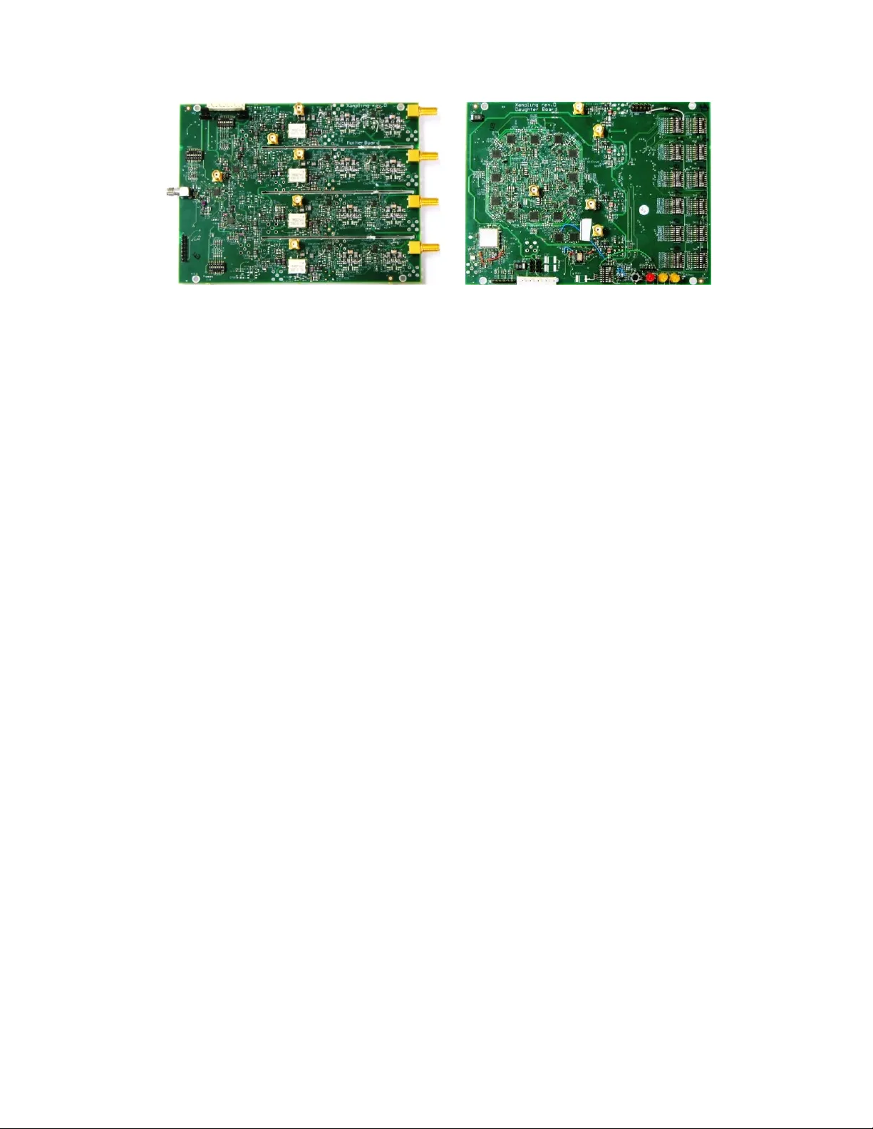
1 Sub-Nyquist Sampling: Bridging Theory and Practice Moshe Mishali and Y onina C. Eldar [ A re vie w of past and recent strategies for sub-Nyquist sampling ] Signal processing methods hav e changed substantially o ver the last se v eral decades. In modern applications, an increasing number of functions is being pushed forward to sophisticated software algorithms, leaving only delicate finely-tuned tasks for the circuit level. Sampling theory , the gate to the digital world, is the key enabling this re v olution, encompassing all aspects related to the con version of continuous-time signals to discrete streams of numbers. The famous Shannon- Nyquist theorem has become a landmark: a mathematical statement which has had one of the most profound impacts on industrial de velopment of digital signal processing (DSP) systems. Over the years, theory and practice in the field of sampling ha ve developed in parallel routes. Contributions by many research groups suggest a multitude of methods, other than uniform sampling, to acquire analog signals [1]–[6]. The math has deepened, leading to abstract signal spaces and innovati ve sampling techniques. W ithin generalized sampling theory , bandlimited signals ha ve no special preference, other than historic. At the same time, the market adhered to the Nyquist paradigm; state-of-the-art analog to digital con v ersion (ADC) devices provide v alues of their input at equalispaced time points [7], [8]. The footprints of Shannon-Nyquist are evident whene ver con version to digital takes place in commercial applications. T oday , sev en decades after Shannon published his landmark result in [9], we are witnessing the outset of an interesting trend. Advances in related fields, such as wideband communication and radio-frequency (RF) technology , open a considerable gap with ADC devices. Conv ersion speeds which are twice the signal’ s maximal frequency component hav e become more and more difficult to obtain. Consequently , alternatives to high rate sampling are drawing considerable attention in both academia and industry . This work has been submitted to the IEEE for possible publication. Copyright may be transferred without notice, after which this version may no longer be accessible. The authors are with the T echnion—Israel Institute of T echnology , Haifa 32000, Israel. Emails: moshiko@tx.technion.ac.il, yonina@ee.technion.ac.il. M. Mishali is supported by the Adams Fellowship Program of the Israel Academy of Sciences and Humanities. Y . C. Eldar is currently on leav e at Stanford, USA. Her work was supported in part by the Israel Science Foundation under Grant no. 170/10 and by the European Commission in the frame work of the FP7 Network of Excellence in W ireless COMmunications NEWCOM++ (contract no. 216715). 2 In this paper , we revie w sampling strategies which target reduction of the ADC rate below Nyquist. Our survey co vers classic works from the early 50’ s of the previous century through recent publications from the past se v eral years. The prime focus is bridging theory and practice, that is to pinpoint the potential of sub-Nyquist strategies to emerge from the math to the hardware. In this spirit, we integrate contemporary theoretical viewpoints, which study signal modeling in a union of subspaces, together with a taste of practical aspects, namely how the av ant-garde modalities boil down to concrete signal processing systems. Our hope is that this presentation style will attract the interest of both researchers and engineers with the aim of promoting the sub- Nyquist premise into practical applications, and encouraging further research into this e xciting ne w frontier . ——— Introduction ——— W e liv e in a digital world. T ele-communication, entertainment, gadgets, business – all rev olve around digital de vices. These miniature sophisticated black-boxes process streams of bits accu- rately at high speeds. Nowadays, electronic consumers feel natural that a media player shows their fav orite movie, or that their surround system synthesizes pure acoustics, as if sitting in the orchestra, and not in the living room. The digital world plays a fundamental role in our e v eryday routine, to such a point that we almost for get that we cannot “hear” or “watch” these streams of bits, running behind the scenes. The world around us is analog, yet almost all modern man-made means for exchanging information are digital. “I am an analog girl in a digital world”, sings Judi Gorman [One Sky , 1998], capturing the essence of the digital rev olution. ADC technology lies at the heart of this revolution. ADC devices translate physical information into a stream of numbers, enabling digital processing by sophisticated software algorithms. The ADC task is inherently intricate: its hardware must hold a snapshot of a fast-v arying input signal steady , while acquiring measurements. Since these measurements are spaced in time, the values between consecutiv e snapshots are lost. In general, therefore, there is no way to recover the analog input unless some prior on its structure is incorporated. A common approach in engineering is to assume that the signal is bandlimited, meaning that the spectral contents are confined to a maximal frequency f max . Bandlimited signals hav e limited (hence slow) time variation, and can therefore be perfectly reconstructed from equali- spaced samples with rate at least 2 f max , termed the Nyquist rate. This fundamental result is often attributed in the engineering community to Shannon-Nyquist [9], [10], although it dates back to earlier works by Whittaker [11] and K otel ´ niko v [12]. 3 x ( t ) Digital Signal Processing ADC x ( nT ) t = nT Nyquist-rate ˆ x ( t ) DA C Analog → Digital Digital → Analog Digital domain Compress / De-Compress Storage media ˆ x ( nT ) Fig. 1: Con ventional blocks in a DSP system. In a typical signal processing system, a Nyquist ADC device provides uniformly-spaced point- wise samples x ( nT ) of the analog input x ( t ) , as depicted in Fig. 1. In the digital domain, the stream of numbers is either processed or stored. Compression is often used to reduce storage volume. DSP , which is unquestionably the crowning glory of this flow , is typically performed on the uncompressed stream. The delicate interaction with the continuous w orld is isolated to the ADC stage, so that sophisticated algorithms can be dev eloped in a flexible software environment. The flow of Fig. 1 ends with a digital to analog (D A C) device which reconstructs x ( t ) from the high Nyquist-rate sequence x ( nT ) . A fundamental reason for processing at the Nyquist rate is the clear relation between the spectrum of x ( t ) and that of x ( nT ) , so that digital operations can be easily substituted for their continuous counterparts. Digital filtering is an e xample where this relation is successfully exploited. Since the power spectral densities of continuous and discrete random processes are associated in a similar manner, estimation and detection of parameters of analog signals can be performed by DSP . In contrast, compression, in general, results in a nonlinear complicated relationship between x ( t ) and the stored data. This paper re vie ws alternati ves to the scheme of Fig. 1, whose common denominator is sampling at a rate below Nyquist. Research on sub-Nyquist sampling spans se veral decades, and has been attracting renewed attention lately , since the growing interest in sampling in union of subspaces, finite rate of innov ation (FRI) models and compressed sensing techniques. Our goal in this surve y is to provide an overvie w of various sub-Nyquist approaches. W e focus this presentation on one- dimensional signals x ( t ) , with applications to wideband communication, channel identification and spectrum analysis. T wo-dimensional imaging applications are also briefly discussed. Throughout, the theme is bridging theory and practice. Therefore, before detailing the specifics of various sub-Nyquist approaches, we first discuss the relation between theory and practice in a broader context. The example of uniform sampling, which without a doubt crossed that bridge, is used to list the essential ingredients of a sampling strategy so that it has the potential to step 4 from math to actual hardware. Our subsequent presentation of sub-Nyquist strategies attempts to gi ve a taste from both worlds – presenting the theoretical principles underlying each strategy and ho w they boil down to concrete and practical schemes. Where relev ant, we shortly elaborate on practical considerations, e.g ., hardware complexity and computational aspects. ——— Essential Ingredients of a Sampling System ——— Nyquist sampling In 1949, Shannon formulated the following theorem for “ a common knowledge in the commu- nication art ” [9, Th. 1]: If a function f ( t ) contains no frequencies higher than W cycles-per -second, it is com- pletely determined by giving its ordinates at a series of points spaced 1 / 2 W seconds apart. It is instructiv e to break this one-sentence formulation into three pieces. The theorem begins by defining an analog signal model – those functions f ( t ) that do not contain frequencies abov e W Hz. Then, it describes the sampling stage, namely pointwise equalispaced samples. In between, and to some extent implicitly , the required rate for this strategy is stated: at least 2 W samples per second. The bandlimited signal model is a natural choice to describe physical properties that are encountered in many applications. For example, a physical communication medium often dictates the maximal frequency that can be reliably transferred. Thus, material, length, dielectric properties, shielding and other electrical parameters define the maximal frequency W . Often, bandlimitedness is enforced by a lo wpass filter with cutof f W , whose purpose is to reject thermal noise be yond frequencies of interest. The implementation suggested by the Shannon-Nyquist theorem, equalispaced pointwise sam- ples of the input, is essentially what industry has been persistently striving to achie ve in ADC design. The sampling stage, per se, is insufficient; The digital stream of numbers needs to be tied together with a reconstruction algorithm. The famous interpolation formula f ( t ) = X n f  n 2 W  sinc(2 W t − n ) , sinc( α ) 4 = sin( π α ) π α , (1) which is described in the proof of [9], completes the picture by providing a concrete reconstruction method. Although (1) theoretically requires infinitely many samples to recover f ( t ) exactly , in practice, truncating the series to a finite number of terms reproduces f ( t ) quite accurately [13]. 5 [T able 1] SUB-NYQUIST SAMPLING: A WISHLIST . Ingredient Requirement Signal model Encountered in applications Sampling rate Approach the minimal for the model at hand Implementation Hardware: Low cost, small number of de vices Software: light computational loads, f ast runtime Robustness React gracefully to design imperf ections Low sensitivity to noise Processing Allow various DSP tasks The theory ensures perfect reconstruction from samples at rate 2 W . A generalized sampling theorem by Papoulis allows to relax design constraints by replacing a single Nyquist-rate ADC by a filter-bank of M branches, each sampled at rate 2 W / M [14]. Another route to design simplification is ov ersampling, which is often used to replace the ideal brickwall filter by more flexible filter designs and to combat noise. Certain ADC designs, such as sigma-delta con version, intentionally ov ersample the input signal, ef fecti vely trading sampling rate for higher quantization precision. Our wishlist, therefore, includes a similar guideline for sub-Nyquist strate gies: achiev e the lo west rate possible in an ideal noiseless setting, and relax design constraints by ov ersampling and parallel architectures. Further to what is stated in the theorem, we believe that tw o additional ingredients motiv ate the widespread use of the Shannon theorem. First, the interpolation formula (1) is rob ust to v arious noise sources: quantization round-off, series truncation and jitter effects [13]. The second appeal of this theorem lies in the ability to shift processing tasks from the analog to the digital domain. DSP is perhaps the major driving force which supports the wide popularity of Nyquist sampling. In sub-Nyquist sampling, the digital stream is, by definition, different from the Nyquist- rate sequence x ( nT ) . Therefore, the challenge of reducing sampling rate creates another obstacle – interfacing the samples with DSP algorithms that are traditionally designed to w ork with the high-rate sequence x ( nT ) , without necessitating interpolation of the Nyquist-rate samples. In other words, we would like to perform DSP at the lo w sampling rate as well. T able 1 summarizes a wishlist for a sub-Nyquist system, based on those properties observ ed in the Shannon theorem. A sampling strategy satisfying most of these properties can, hopefully , find its way into practical applications. Architectur e of a sub-Nyquist system A high-le vel architecture of a sub-Nyquist system is depicted in Fig. 2, following the spirit of the traditional block diagram of Fig. 1. The ADC task is carried out by some hardware mechanism, which outputs a sequence y [ n ] of measurements at a low rate. Since the sub-Nyquist samples y [ n ] are, by definition, different from the uniform Nyquist sequence x ( nT ) of Fig. 1, a digital core may be needed to preprocess the raw data before DSP can take place. A prominent advantage over 6 x ( t ) Signal Processing y [ n ] Low-rate ˆ x ( t ) Analog → Digital Digital → Analog Digital domain Storage media ˆ y [ n ] Sub-Nyquist Hardware Digital core Low-rate Low-rate Sub-Nyquist Reconstruction Fig. 2: A high-lev el architecture of a sub-Nyquist system. Both processing and continuous recovery are based on lowrate computations. The ra w data can be directly stored. con ventional Nyquist architectures is that the DSP operations are carried out at the low input rate. The digital core may also be needed to assist in reconstructing x ( t ) from y [ n ] . Another adv antage is that storage may not require a preceding compression stage; conceptually , the compression has already been performed by the sub-Nyquist sampling hardware. An important point we would like to emphasize is that strictly speaking, none of the methods we surve y actually breach the Shannon-Nyquist theorem. Sub-Nyquist techniques leverage known signal structure, that goes beyond kno wledge of the maximal frequency component. The key to de veloping interesting sub-Nyquist strategies is to rely on structure that is not too limiting and still allows for a broad class of signals on the one hand, while enabling sampling rate reduction on the other . One of the earlier examples demonstrating how signal structure can lead to rate reduction is sampling of multiband signals with kno wn center frequencies, namely , signals that consists of sev eral known frequenc y bands. W e begin our revie w with this classic setting. W e then discuss more recent paradigms which enable sampling rate reduction e ven when the band positions are unknown. As we show , this setting is a special case of a more general class of signal structures known as unions of subspaces, which includes a variety of interesting examples. After introducing this general model, we consider se veral sub-Nyquist techniques which e xploit such signal structure in sophisticated ways. ——— Classic Sub-Nyquist Methods ——— In this section we survey classic sampling techniques which reduce the sampling rate belo w Nyquist, assuming a multiband signal with known frequency support. An example of a multiband input with N bands is depicted in Fig. 3, with individual bandwidths not greater than B Hz, centered around carrier frequencies f i ≤ f max ( N is even for real-valued inputs). Since the carriers f i are known and the spectral support is fixed, the set of multiband inputs on that support is closed under linear combinations, thereby forming a subspace of possible inputs. Overlapping bands are 7 f 1 B f 2 f 3 f 1 B f 2 f 3 f − f 1 − f 2 − f 3 Receiver f max Fig. 3: Three RF transmissions with different carriers f i . The receiv er sees a multiband signal (bottom drawing). Fig. 4: A block diagram of a typical I-Q demodulator . permitted, though in practical scenarios, e.g., communication signals, the bands typically do not ov erlap. Demodulation The most common practice to av oid sampling at the Nyquist rate, f NYQ = 2 f max , (2) is demodulation. The signal x ( t ) is multiplied by the carrier frequency f i of a band of interest, so as to shift contents of a single narrowband transmission from high frequencies to the origin. This multiplication also creates a narro wband image around 2 f i . Lo wpass filtering is used to retain only the baseband version, which is subsequently sampled uniformly in time. This procedure is carried out for each band indi vidually . Demodulation provides the DSP block with the information encoded in a band of interest. T o make this statement more precise, we recall how modern communication is often performed. T wo B / 2 -bandlimited information signals I ( t ) , Q ( t ) are modulated on a carrier frequenc y f i with a relati ve phase shift of 90 ◦ . The quadrature output signal is then gi ven by [15] r i ( t ) = I ( t ) cos(2 π f i t ) + Q ( t ) sin(2 π f i t ) . (3) For example, in amplitude modulation (AM), the information of interest is the amplitude of I ( t ) , while Q ( t ) = 0 . Phase- and frequency-modulation (PM/FM) obe y (3) such that the analog message is g ( t ) = arctan( I ( t ) /Q ( t )) [16]. In digital communication, e .g., phase- or frequency shift-ke ying (PSK/FSK), I ( t ) , Q ( t ) carry symbols. Each symbol encodes one, two or more 0/1 bits. The I/Q-demodulator , depicted in Fig. 4, basically rev erts the actions performed at the transmitter side which constructed r i ( t ) . Once I ( t ) , Q ( t ) are obtained by the hardware, a pair of lowrate ADC de vices acquire uniform samples at rate B . The subsequent DSP block can infer the analog message or decode the bits from the recei ved symbols. Reconstruction of each r i ( t ) , and consequently recov ery of the multiband input x ( t ) , is as 8 1 2 3 4 5 6 7 8 9 10 0 1 2 3 4 5 6 7 8 9 10 Fig. 5: The allo wed (white) and forbidden (gray) undersampling rates of a bandpass signal depend on its spectral position [18]. simple as remodulating the information on their carrier frequencies f i , according to (3). This option is used in relay stations or regenerati ve repeaters which decode the information I ( t ) , Q ( t ) , use digital error correction algorithms, and then transform the signal back to high frequencies for the next transmission section [17]. I/Q demodulation has dif ferent names in the literature: zero-IF recei ver , direct con version, or homodyne; cf. [15] for various demodulation topologies. Each band of interest requires 2 hardware channels to extract the relev ant I ( t ) , Q ( t ) signals. A similar principle is used in lo w-IF receiv ers, which demodulate a band of interest to low frequencies b ut not around the origin. Low-IF recei vers require only one hardware channel per band, though the sampling rate is higher compared to zero- IF recei vers. Undersampling ADC Aliasing is often considered an undesired ef fect of sampling. Indeed, when a bandlimited signal is sampled below its Nyquist rate, aliases of high-frequency content trample information located around other spectral locations and destroy the ability to recov er the input. Undersampling ( a.k.a., direct bandpass sampling) refers to uniform sampling of a bandpass signal at a rate lo wer than the maximal frequency , in which case proper sampling rate selection renders aliasing advantageous. Consider a bandpass input x ( t ) whose information band lies in the frequency range ( f l , f u ) of length B = f u − f l . In this case, the lowest rate possible is 2 B [19]. Uniform sampling of x ( t ) at a rate of f s that obeys 2 f u k ≤ f s ≤ 2 f l k − 1 , (4) 9 for some integer 1 ≤ k ≤ f u /B , ensures that aliases of the positiv e and negati ve contents do not ov erlap [18]. Fig. 5 illustrates the valid sampling rates implied by (4). In particular , the figure and (4) show that f s = 2 B is achiev ed only if x ( t ) has an inte ger band positioning, f u = k B . Furthermore, as the rate reduction factor k increases, the valid region of sampling rates becomes narro wer . For a giv en band position f u , the region corresponding to the maximal k ≤ f u /B is the most sensitiv e to slight deviations in the exact values of f s , f l , f u [18]. Consequently , besides the fact that f s = 2 B cannot be achiev ed in general (ev en in ideal noiseless settings), a significantly higher rate is likely to be required in practice in order to cope with design imperfections. Bridging theory and practice, the fact that (4) allows rate reduction, e ven though higher than the minimal, is useful in many applications. In undersampling, the ADC is applied directly to x ( t ) with no preceding analog preprocessing components, in contrary to the RF hardware used in I/Q demodulation. Howe v er , not every ADC de vice fits an undersampling system: only those devices whose front-end analog bandwidth exceeds f u are viable. Box 1 expands on this constraint of front-end bandwidth in Nyquist and undersampling ADCs. Box 1. Nyquist and Undersampling ADC Devices An ADC device, in the most basic form, repeatedly alternates between two states: track- and-hold (T/H) and quantization. During T/H, the ADC tracks the signal v ariation. When an accurate track is accomplished, the ADC holds the value steady so that the quantizer can con vert the value into a finite representation. Both operations must end before the next signal v alue is acquired. In the signal processing community , an ADC is often modeled as an ideal pointwise sampler that captures values of x ( t ) at a constant rate of r samples per second. As with any analog circuitry , the T/H function is limited in the range of frequencies it can accept: a lowpass filter with cutof f b can be used to model the T/H capability [20]. In most off-the-shelf ADCs, the analog bandwidth parameter b is specified higher than the maximal sampling rate r of the device. The table lists example de vices. When using an ADC at the Nyquist rate of the input, the filter can be omitted from the model, since the signal is 10 bandlimited to f max = r / 2 ≤ b . In contrast, for sub-Nyquist purposes, the analog bandwidth b becomes an important factor in accurate modeling and actual selection of the ADC, since it defines the maximal input frequency that can be undersampled: f max ≤ b. (5) T ypically , b specifies the − 3 dB point of the T/H frequency response. Thus, if flat response in the passband is of interest, f max cannot approach too close to b . F or example, if x ( t ) is a bandpass signal in the range [600 , 625] MHz, then undersampling at rate f s = 50 MHz satisfies condition (4). In this example, whilst both AD9433 and AD10200 are capable of sampling at a rate r ≥ 50 MHz, only the former is applicable due to (5). Undersampling ADCs have a wider spacing between consecuti ve samples. This adv antage is translated into simplifying design constraints, especially in the duration allo wed for quantization. Howe v er , regardless of the sampling rate r , the T/H stage must still hold a pointwise value of a fast-v arying signal. In terms of analog bandwidth there is no substantial dif ference between Nyquist and undersampling ADCs; both have to accommodate the Nyquist rate of the input. Undersampling has two prominent dra wbacks. First, the resulting rate reduction is generally significantly higher than the minimal as evident from Fig. 5. As listed in T able 1, approaching the minimal rate, at least theoretically , is a desired property . Second, and more importantly , undersampling is not suited to multiband inputs. In this scenario, each individual band defines a range of valid values for f s according to (4). The sampling rate must be chosen in the intersection of these conditions. Moreover , it should also be verified that the aliases due to the different bands do not interfere. As noted in [21], satisfying all these constraints simultaneously , if possible, is likely to require a considerable rate increase. Periodic nonuniform sampling The discussion above suggests that uniform sampling may not be the most desirable acquisition strategy for inputs with multiband structure, unless sufficient analog hardware is used as in Fig. 4. Classic studies in sampling theory hav e focused on nonuniform alternativ es. In 1967, Landau prov ed a lower bound on the sampling rate required for spectrally-sparse signals [19] with known frequency support when using pointwise sampling. In particular , Landau’ s theorem supports the intuiti ve expectation that a multiband signal x ( t ) with N information bands of individual widths B necessitates a sampling rate no lower than the sum of the band widths, i.e., N B . 11 Fig. 6: Second-order PNS. The bandpass signal x ( t ) is sampled by two rate- B uniform sequences with relativ e time delay φ . The interpolation filters cancel out the contribution of the undesired alias. Periodic nonuniform sampling (PNS) allows to approach the minimal rate N B without com- plicated analog preprocessing. Besides ADC devices, the hardware needs only a set of time-delay elements. PNS consists of m undersampling sequences with relati ve time-shifts: y i [ n ] = x ( nT s + φ i ) , 1 ≤ i ≤ m, (6) such that the total sampling rate m/T s is lower than f NYQ . Kohlenber g [22] was the first to prov e perfect reco very of a bandpass signal from PNS samples taken at an a v erage rate of 2 B samples/sec. Lin and V aidyanathan [23] extended his approach to multiband signals. W e follow the presentation in [23] and explain how the parameters m, T s , φ i are chosen in the simpler case of a bandpass input. Suppose x ( t ) is supported on I = ( f l , f u ) ∪ ( − f u , − f l ) and B = f u − f l . W e choose a PNS system with m = 2 channels ( a.k.a., second-order PNS), a sampling interval T s = 1 /B , φ 1 = 0 and φ 2 = φ . Due to the undersampling in each channel, aliases of the band contents tile the spectrum, so that the positiv e and ne gati ve images fold on each other , as visualized in Fig. 6. In the frequency domain, the sample sequences (6) satisfy a linear system [23] T s Y 1 ( f ) = X ( f ) + X ( f − β ( f ) B ) , (7a) T s Y 2 ( f ) = X ( f ) + X ( f − β ( f ) B ) e − j 2 π β ( f ) φB , (7b) for f ∈ I . The function β ( f ) = − β ( − f ) is piece wise constant over f ∈ I , inde xing the aliased images. The exact levels and transitions of β ( f ) depend explicitly on the band position as shown 12 in Fig. 6. The aliases have unity weights in y 1 [ n ] , whereas the time delay φ in y 2 [ n ] results in unequal weighting. System (7) is linearly independent as long as φ obeys e − j 2 π β ( f ) φB 6 = 1 . (8) Since β ( f ) can take on only 4 distinct values within f ∈ ( f l , f u ) , there are many possible selections for φ which satisfy (8). Recov ery of x ( t ) is carried out by interpolation [22], [23] x ( t ) = X n ∈ Z y 1 [ n ] g 1 ( t − nT s ) + y 2 [ n ] g 2 ( t − nT s ) , (9) with bandpass filters g 1 ( t ) , g 2 ( t ) , which re verse the weights in (7). These filters ha ve frequency responses G 1 ( f ) = 1 1 − e − j 2 π β ( f ) φB , G 2 ( f ) = − G 1 ( f ) , f ∈ I , (10) as are drawn in Fig. 6. In practice, these filters can be realized digitally , so that the output of Fig. 6 is the Nyquist-rate sequence x ( nT ) , with T = 1 / 2 f u equal to the Nyquist interval. Subsequently , a D AC device may interpolate the continuous signal x ( t ) . The extension to multiband signals with N bands of individual widths B is accomplished follo wing the same procedure using an N th order PNS system, with delays φ l , 1 ≤ l ≤ N [23]. Reconstruction consists of N filters, which are piecewise constant over the frequency support of x ( t ) . The indexing function β ( f ) is extended to an N × N matrix A ( f ) , with entries depending on φ l and band locations. In general, an N th-order PNS can resolv e up to N aliases, since it provides a set of N equations. The equations are linearly independent, or solvable, if A − 1 ( f ) exists ov er the entire multiband support [23]. Lin and V aidyanathan show that the choice φ l = lφ renders A ( f ) a V andermonde matrix, in which case the choice of the single delay φ is tractable. Bands of dif ferent widths are treated by viewing the bands as consisting of narrower intervals which are integer multiplies of a common length. For example, if N = 4 (two transmissions) and B 1 = k 1 B , B 2 = k 2 B , then the equiv alent model has 4( k 1 + k 2 ) bands of equal width B . This conceptual step allo ws to achie ve the Landau rate. For technical completeness, the same solution applies to mixed rational-irrational bandwidths for an infinitesimal rate increase. PNS vs. demodulation An apparent adv antage of PNS ov er RF demodulation is that it can approach Landau’ s rate with no hardware components preceding the ADC de vice. This theoretical advantage, ho we v er , was not widely embraced by industry for acquisition of multiband inputs. In an attempt to reason this situation, we lev erage practical insights from time-interlea ving ADCs, a popular design topology 13 T/H Q nt. T/H Q nt. T/H Q nt. Fig. 7: Block diagram of a time-interlea ved ADC. used in high-speed con verters [24]–[26]. T ime-interlea ved ADC technology splits the task of con verting a wideband signal into M parallel branches, essentially utilizing Papoulis’ theorem with a bank of time-delay elements. Each branch in the block diagram of Fig. 7 introduces a time delay of φ l seconds and subsequently samples x ( t − φ l ) at rate 1 / M T , where T = 1 /f NYQ is the Nyquist interval. Ideally , when φ l = l T , interleaving the M digital streams provides a sequence that coincides with the Nyquist rate samples x ( nT ) . A time-interlea ving ADC consists of M separate T/H circuitries and quantizers, thereby relaxing design constraints by allowing each branch to perform the conv ersion task in a duration of M T seconds rather than T . Whilst the larger duration simplifies quantization, the T/H complexity remains almost the same – it still needs to track a Nyquist-rate varying input and hold its v alue at a certain time point, reg ardless of the higher duration allocated for conv ersion, as explained in Box 1. PNS is a degenerated time-interlea ved ADC with only m < M branches. This means that a PNS-based sub-Nyquist solution requires Nyquist-rate T/H circuitries, one per sampling branch. In addition to high analog bandwidth, PNS also requires compensating for imperfect production of the time delay elements. Consequently , realizing PNS in practice may not be much easier than designing an M -channel time-interleaved ADC with Nyquist-rate sampling capabilities. Thus, while time-interleaving is a popular design method for Nyquist ADCs, it may be less useful for the purpose of sub-Nyquist sampling of wideband signals with large f NYQ . More broadly , any pointwise strategy , which is applied directly on a wideband signal, has a technological barrier around the maximal rate of commercial T/H circuitry . This barrier creates an (undesired) coupling between advances in RF and ADC technologies; as transmission frequencies gro w higher , a comparable speed-up of T/H bandwidth is required. W ith accelerated dev elopment of RF devices, a considerable gap has already been opened, rendering ADCs a bottleneck in many modern signal processing applications. In contrast, in demodulation, even though the signal 14 Multiband communication Union o v er possible band p ositions f i ∈ [0 , f max ] f 0 f 1 f i f 2 f max FM QAM BPSK t t 1 a 1 t 2 a 2 t 3 a 3 t 0 1 h ( t ) τ F ading c hannel Time-dela y estimation Union o v er p ossible path dela ys t i ∈ [0 , τ ] Fig. 8: Example applications of UoS modeling. is wideband, an ADC with lo w analog bandwidth is sufficient due to the preceding lo wpass filter . RF preprocessing (mixers and filters) b uf fer between x ( t ) and actual ADCs, thereby offering a scalable sampling solution, which effecti v ely decouples T/H capabilities from dependency on the input’ s maximal frequency . More importantly , demodulation ensures that only in-band noise enters the system, whereas in PNS, out-of-band noise from the entire Nyquist bandwidth is aggregated. W e no w turn to revie w sub-Nyquist techniques when the carrier frequencies are unkno wn, as well as low rate sampling strategies for other interesting analog models. The insights we gathered so far hint that analog preprocessing is an advantageous route tow ards developing efficient sub- Nyquist strategies. ——— Union of Subspaces ——— Motivation Demodulation, a classic sub-Nyquist strategy , assumes an input signal which lies in certain interv als within the Nyquist range. But, what if the input signal is not limited to a predefined frequency support, or e ven worse if it spans the entire Nyquist range – can we still reduce the sampling rate belo w Nyquist? Perhaps surprising, we shall see in the sequel that the answer is af firmati ve, pro vided that the input has additional structure we can exploit. Figure 8 illustrates two such scenarios. Consider for e xample the scenario of a multiband input x ( t ) with unkno wn spectral support, consisting of N frequenc y bands of individual widths no greater than B Hz. In contrast to the classic setup, the carrier frequencies f i are unkno wn, and we are interested in sampling such multiband inputs with transmissions located anywhere belo w f max . At first sight, it may seem that sampling at the Nyquist rate f NYQ = 2 f max is necessary , since e very frequency interval below f max appears in the support of some multiband x ( t ) . On the other hand, since each specific x ( t ) in this model has structure – it fills only a portion of the Nyquist range (only N B Hz) – we intuiti vely expect to be able to reduce the sampling rate below f NYQ . 15 Another interesting problem is sampling of signals which consist of several echoes of a known pulse shape, where the delays and attenuations are a-priori unkno wn. Mathematically , x ( t ) = L X ` =1 a ` h ( t − t ` ) , t ∈ [0 , τ ] , (11) for some given pulse shape h ( t ) and unknown t ` , a ` . Signals of this type belong to the broader family of FRI signals, originally introduced by V etterli et al. in [27], [28]. Echoes are encountered, for example, in multipath fading communication channels. The transmitter can assist the receiv er in channel identification by sending a short probing pulse h ( t ) , based on which the receiver can resolve the fading delays t ` and use this information to decode subsequent information messages. In radar applications, inputs of the form (11) are prev alent, where the delays t ` correspond to the unkno wn locations of targets in space, while the amplitudes a ` encode Doppler shifts indicating target speeds. Medical imaging techniques, e.g., ultrasound, record signals that are structured according to (11) when probing density changes in human tissue. Underwater acoustics also conform with (11). The common denominator of these applications is that h ( t ) is a short pulse in time, so that the bandwidth of h ( t ) , and consequently that of x ( t ) , spans a large Nyquist range. Nonetheless, giv en the structure (11), we can intuitively expect to determine x ( t ) from samples at the rate of innov ation, namely 2 L samples per τ , which counts the actual number of unknowns, t ` , a ` , 1 ≤ ` ≤ L in ev ery interv al. These examples hint at a more general notion of sub-Nyquist sampling, in which the underlying signal structure is utilized to reduce acquisition rate below the apparent input bandwidth. As a special case, this notion includes the classic settings of structure gi ven by a predefined frequency support. T o capture more general structures, we present next the union of subspace (UoS) model, originally proposed by Lu and Do in [29]. Mathematical framework Denote by x ( t ) an analog signal in the Hilbert space H = L 2 ( R ) , which lies in a parameterized family of subspaces x ( t ) ∈ U 4 = [ λ ∈ Λ A λ , (12) where Λ is an index set, and each individual A λ is a subspace of H . The ke y property of the UoS model (12) is that the input x ( t ) resides within A λ ∗ for some λ ∗ ∈ Λ , but a-priori, the exact subspace index λ ∗ is unkno wn. W e define the dimension (or bandwidth) of U as the dimension of its affine hull Σ , namely the space of all linear combinations of x ( t ) ∈ U . T ypically , the union U has dimension that is relatively high compared with those of the individual subspaces A λ . Multiband signals with unkno wn carriers f i can be described by (12), where each A λ corre- 16 sponds to signals with specific carrier positions and the union is taken ov er all possible f i ∈ [0 , f max ] . In this case, each A λ has effecti ve bandwidth N B , whereas the union U has f max bandwidth, as follows from the definition of Σ . Similarly , echoes with unkno wn time-delays of the form (11) correspond to L -dimensional subspaces A λ that capture the amplitudes a ` . A union over all possible delays t l ∈ [0 , τ ] provides an efficient way to group these infinitely-many subspaces to a single set U . The large bandwidth of h ( t ) results in U with a high Nyquist bandwidth. Union modeling sheds new light on sampling below the Nyquist rate. Sub-Nyquist in the union setting, conceptually , consists of two layers of rate reduction: from the dimensions of U to that of the individual subspaces A λ , and then, further reduction within the scope of a single subspace until reaching its ef fecti ve bandwidth (rather than twice its highest frequency component). The second layer is essentially what is treated in the classic works surveyed earlier , which considered a single subspace defined according to a giv en spectral support. Eventually , the tricky part is how to design sampling strategies that combine these reduction steps and achiev e the minimal rate by one con version stage. Box 2 expands on the challenges of sampling union sets. The model (12) can be categorized to four types, according to the cardinality of Λ (finite or infinite) and the dimensions of the individual subspaces A λ (finite or infinite). In the next sections, we re vie w sub-Nyquist sampling methods for se veral prototype union models (categorized hereafter by the dimensions pair λ − A λ , where “F” abbre viates finite): • multiband with unkno wn carrier positions (type F − ∞ ), • v ariants of FRI models (cov er two union types: ∞ − F and ∞ − ∞ ), and • a sparse sum of harmonic sinusoids (type F − F). A solution for sampling and reconstruction was de v eloped in [30] for more general F − F union structures. A special case of the F − F case is the sparsity model underlying compressed sensing [31], [32]. In this re vie w , ho wev er , our prime focus is analog signals which exhibit infiniteness in either Λ or A Λ . A more detailed treatment of the general union setting can be found in [33], [34]. Box 2. Generalized Sampling in Union of Subspaces Generalized sampling theory extends upon pointwise acquisition by viewing the measure- ments as inner products [3]–[6], [35], y [ n ] = h x ( t ) , s n ( t ) i , n ∈ Z , (13) between an input signal x ( t ) and a set of sampling functions s n ( t ) . Geometrically , the sample 17 sequence y [ n ] is obtained by projecting x ( t ) onto the space S = span { s n ( t ) | n ∈ Z } . (14) A special case is of a shift-inv ariant space S spanned by s n ( t ) = s ( t − nT ) for some generator function s ( t ) [5]. In this scenario, (13) amounts to filtering x ( t ) by s ( − t ) and taking pointwise samples of the output e very T seconds. T raditional pointwise acquisition y [ n ] = x ( nT ) corresponds to a shift-inv ariant S with a Dirac generator s ( t ) = δ ( t ) . Multichannel sampling schemes correspond to a shift-in v ariant space S spanned by shifts of multiple generators [36], [37]. Theory and applications of subspace sampling were widely studied ov er the years. If x ( t ) resides within a subspace A ⊆ H of an ambient Hilbert space H , then the samples (13) determine the input whene ver the orthogonal complement A ⊥ satisfies a direct sum condition [6] A ⊥ ⊕ S = H . (15) Reconstruction is obtained by an oblique projection [6]. Roughly speaking, in noiseless settings, perfect recovery is possible whenever the angle θ between the subspaces A , S is dif ferent than 90 ◦ , and robustness to noise increases as θ tends to zero. U n io n of su b space s Sa m pli n g space Si n gle su b space When x ( t ) lies in a union of subspaces (12), both theory and practice become more intricate. For instance, ev en if the angles between S and each of the subspaces A λ are sufficiently small, the samples may not determine the input if several subspaces are too close to each other; see the illustration. Recent studies [29] hav e shown that (13) is stably in vertible if (and only if) there exist constants 0 < α < β < ∞ such that α k x 1 ( t ) − x 2 ( t ) k 2 H ≤ k y 1 [ n ] − y 2 [ n ] k 2 l 2 ≤ β k x 1 ( t ) − x 2 ( t ) k 2 H , (16) for ev ery signals x 1 ( t ) , x 2 ( t ) ∈ A λ 1 + A λ 2 and for all possible pairs of λ 1 , λ 2 . In practice, 18 sampling methods for specific union applications use certain hardware constraints to hint at preferred selections of stable sampling functions s n ( t ) ; see for example [20], [27], [38]–[41] and other UoS methods surve yed in this re vie w . ——— Multiband Signals with Unknown Carrier F requencies ——— Union modeling A description of a multiband union can be obtained by letting λ = { f i } , so that each choice of carrier positions f i determines a single subspace A λ in U . In principle, f i lies in the continuum f i ∈ [0 , f max ] , resulting in union type ∞ − ∞ containing infinitely many subspaces. In the setup we describe below a different viewpoint is used to treat the multiband model as a finite union of bandpass subspaces (type F − ∞ ), termed spectrum slices [20], [42]. In this vie wpoint, the Nyquist range [ − f max , f max ] is conceptually di vided into M = 2 L + 1 consecutiv e, non-overlapping, slices of individual widths f p , such that M f p ≥ 2 f max . Each spectrum slice represents a single bandpass subspace. By choosing f p ≥ B , we ensure that no more than 2 N spectrum slices are active, namely contain signal energy . In this setting, there are  M 2 N  subspaces in U . Dividing the spectrum to slices is only a conceptual step, which assumes no specific displacement with respect to the band positions. The adv antage of this viewpoint is that switching to union type F − ∞ simplifies the digital reconstruction algorithms, while preserving a degree of infiniteness in the dimensions of each individual subspace A λ . Semi- and fully-blind pointwise approaches Earlier approaches for treating multiband signals with unknown carriers were semi-blind: a sampler design independent of band positions combined with a reconstruction algorithm that requires exact support kno wledge. Herley et al. [43] and Bresler et al. [44], [45] studied multi- coset sampling, a PNS grid that is a subset of the Nyquist grid, and proved that the grid points can be selected independently of the band positions. The reconstruction algorithms in [43], [45] coincide with the non-blind PNS reconstruction algorithm of [23], for time-delays φ l chosen on the Nyquist grid. These works approach the Landau rate, namely N B samples/sec. Other techniques targeted the rate N B by imposing alternati ve constraints on the input spectrum [44]. Recently , the math and algorithms for fully-blind systems were dev eloped in [39], [42], [46]. In this setting, both sampling and reconstruction operate without knowledge of the band positions. A fundamental distinction between non- or semi-blind approaches to fully-blind systems is that the 19 minimal sampling rate increases to 2 N B , as a consequence of recov ery which lacks knowledge on the exact spectral support. A more thorough discussion in [42] studies the differences between earlier approaches that were based on subspace modeling and the fully-blind sampling methods [39], [42], [46] that are based on union modeling. Box 3 revie ws the theorems underlying this distinction. The fully-blind framework dev eloped in [42], [46] provides reconstruction algorithms that can be combined with various sub-Nyquist sampling strategies: multi-coset in [42], filter- bank follo wed by uniform sampling in [39] and the modulated wideband con v erter (MWC) in [20]. In viewing our goal of bridging theory and practice, the Achilles heel of the combination with multi-coset is pointwise acquisition, which enters the Nyquist-rate thru the backdoor of T/H bandwidth. As discussed earlier and outlined in Box 1, pointwise acquisition requires an ADC de vice with Nyquist-bandwidth T/H circuitry . The filter-bank approach is part of a general frame work de veloped in [39] for treating analog signals lying in a sparse-sum of shift-in variant (SI) subspaces, which includes multiband with unknown carriers as a special case. The filters and ADCs, ho we ver , also require Nyquist-rate bandwidth, in this setting. In the next section, we describe the MWC strategy , which utilizes the principles of the fully- blind sampling framew ork, and also results in a hardware-efficient sub-Nyquist strategy that does not suffer from analog bandwidth limitations of T/H technology . In essence, the MWC extends con ventional I/Q demodulation to multiband inputs with unkno wn carriers, and as such it also provides a scalable solution which decouples undesired RF-ADC dependencies. The combination of hardw are-ef ficient sampler with fully-blind reconstruction ef fectiv ely satisfies the wishlist of T able 1. Box 3. Universal Bounds on Sub-Nyquist Sampling Rates Sampling strategies are often compared on the basis of the required sampling rate. It is therefore instructiv e to compare existing strategies with the lowest sampling rate possible. For instance, the Shannon-Nyquist theorem states (and achie ves) the minimal rate 2 f max for bandlimited signals. The following results derive the lo west sub-Nyquist sampling rates for spectrally-sparse signals, under either subspace or union of subspace priors. Consider the case of a subspace model for signals that are supported on a fixed set I of frequencies: B I = { x ( t ) ∈ L 2 ( R ) | supp X ( f ) ⊆ I } . (17) A grid R = { t n } of time points is called a sampling set for B I if the sequence of samples 20 x R [ n ] = x ( t n ) is stable, namely there exist constants α > 0 and β < ∞ such that: α k x ( t ) − y ( t ) k 2 L 2 ≤ k x R [ n ] − y R [ n ] k 2 l 2 ≤ β k x ( t ) − y ( t ) k 2 L 2 , ∀ x ( t ) , y ( t ) ∈ B I . (18) Landau [19] prov ed that if R is a sampling set for B I then it must hav e a density D − ( R ) 4 = lim r →∞ inf y ∈ R | R ∩ [ y , y + r ] | r ≥ meas( I ) , (19) where D − ( R ) is the lower Beurling density and meas( I ) is the Lebesgue measure of I . The numerator in (19) counts the number of points from R in ev ery interval of width r of the real axis. The Beurling density (19) reduces to the usual concept of avera ge sampling rate for uniform and periodic nonuniform sampling. Consequently , for multiband signals with N bands of widths B , the minimal sampling rate is the sum of the bandwidths N B , gi ven a fixed subspace description of known band locations. A union of subspaces model can describe a more general scenario, in which, a-priori, only the fraction 0 < Ω < 1 of the Nyquist bandwidth actually occupied is assumed kno wn b ut not the band locations: N Ω = { x ( t ) ∈ L 2 ( R ) | meas (supp X ( f )) ≤ Ω f NYQ } . (20) A blind sampling set R for N Ω is stable if there exists α > 0 and β < ∞ such that (18) holds with respect to all signals from N Ω . A theorem of [42] deriv ed the minimal rate requirement for the set N Ω : D − ( R ) ≥ min { 2Ω f NYQ , f NYQ } . (21) This requirement doubles the minimal sampling rate to 2 N B for multiband signals whose band locations are unknown. It also implies that if the occupation Ω > 50% , then no rate reduction is possible. Both minimal rate theorems are uni v ersal for pointwise sampling strate gies in the sense that for any choice of a grid R = { t n } , if the av erage rate is too low , namely below (19) or (21), then there exist signals whose samples on R are indistinguishable. Note that both results are nonconstructi ve; they do not hint at a sampling strategy that achiev es the minimal rate. Modulated wideband conv erter The MWC [20] combines the advantages of RF demodulation and the blind recovery ideas de veloped in [42], and allo ws sampling and reconstruction without requiring kno wledge of the 21 band locations. T o circumvent analog bandwidth issues in the ADCs, an RF front-end mixes the input with periodic wav eforms. This operation imitates the ef fect of delayed undersampling, namely folding the spectrum to baseband with dif ferent weights for each frequenc y interval. In contrast to undersampling (or PNS), aliasing is realized by RF components rather than by taking adv antage of the T/H circuitry . In this way , bandwidth requirements are shifted from ADC devices to RF mixing circuitries. The key idea is that periodic mixing serves another goal – both the sampling and reconstruction stages do not require kno wledge of the carrier positions. Before describing the MWC system that is depicted in Fig. 9, we point out se veral properties of this approach. The system is modular; Sampling is carried out in independent channels, so that the rate can be adjusted to match the requirements of either a traditional subspace model or the more challenging union of subspace prior . It can also scale up to the Nyquist rate to support the standard Shannon-Nyquist bandlimited prior . The reconstruction algorithm that appears in Fig. 12 has se veral functional blocks: detecting the spectral support thru a computationally light optimization problem, signal reco very and information e xtraction. Support detection, the heart of this digital algorithm, is carried out whene ver the carrier locations v ary . The rest of the digital computations are simple and performed in real-time. In addition, the recovery stage outputs baseband samples of I ( t ) , Q ( t ) . This enables a seamless interface to existing DSP algorithms with sub-Nyquist processing rates, as could have been obtained by classic demodulation had the carriers f i been kno wn. W e now elaborate on each part of this strategy . Sub-Nyquist sampling scheme The con version from analog to digital consists of a front-end of m channels, as depicted in Fig. 9. In the i th channel, x ( t ) is multiplied by a periodic wav eform p i ( t ) with period T p = 1 /f p , lo wpass filtered by h ( t ) , and then sampled at rate f s = 1 /T s . The figure lists basic and adv anced configurations. T o simplify , we concentrate on the theory underlying the basic version, in which the sampling interval T s equals the aliasing period T p , each channel samples at rate f s ≥ B and the number of hardware branches m ≥ 2 N , so that the total sampling rate can be as lo w as 2 N B . These choices stem from necessary and suf ficient conditions deri ved in [20] on the required sampling rate mf s to allow perfect reconstruction. If the input’ s spectral support is known, then the same conditions translate to a similar parameter choice with half the number of channels, resulting in a total sampling rate as low as N B . Thus, although the MWC does not take pointwise values of x ( t ) , its optimal sampling rate coincides with the lowest possible rates by pointwise strategies, which are discussed in Box 3. Adv anced configurations enable additional hardw are sa vings by collapsing the number of branches m by a factor of q at the expense of increasing the sampling rate of each channel by the same factor , ultimately enabling a single-channel sampling system [20]. 22 y i [ n ] h ( t ) p 1 ( t ) h ( t ) p m ( t ) x ( t ) y m [ n ] y 1 [ n ] Lowpass t = nT s T p -perio dic 1 /T s p i ( t ) RF front-end Lowrate ADC (Low analog bandwidth) Analog → Digital Parameter/Configuration Basic Adv anced # channels m ≥ 4 N ≥ 2 N/q # p eriodic generators = m 1 Aliasing rate 1 /T p ≥ B ≥ B Cutoff / channel rate 1 /T s = 1 /T p = q/T p T otal rate approach 4 N B approach 2 N B Fig. 9: Block diagram of the modulated wideband con verter [20]. The table at the bottom lists the parameters choice of the basic and advanced MWC configurations. Adapted from [47], c  [2011] IET . f 0 max f f p lf p ¯ lf p ˜ lf p + c il c i ¯ l c i ˜ l Spectrum of x ( t ) Spectrum of y i [ n ] Spectrum of y i 0 [ n ] + c i 0 l c i 0 ¯ l c i 0 ˜ l B Fig. 10: The spectrum slices from x ( t ) are ov erlayed in the spectrum of the output sequences y i [ n ] . In the example, channels i and i 0 realize different linear combinations of the spectrum slices centered around lf p , ¯ lf p , ˜ lf p . For simplicity , the aliasing of the negati ve frequencies is not dra wn. Adapted from [47], c  [2011] IET . This technique is also briefly re vie wed in the next subsection. The choice of periodic waveforms p i ( t ) becomes clear once analyzing the ef fect of periodic mixing. Each p i ( t ) is periodic, and thus has a Fourier expansion p i ( t ) = ∞ X l = −∞ c il e j 2 π f p lt . (22) Denote by z l [ n ] the sequence that would hav e been obtained by mixing x ( t ) with e j 2 π f p lt , filtering by h ( t ) and sampling every T seconds. By superposition, mixing x ( t ) by the sum in (22) outputs y i [ n ] which is a linear combination of the z l [ n ] sequences according to the Fourier coef ficients c il of p i ( t ) . Fig. 10 visualizes the ef fect of mixing with periodic w a veforms, where each sequence z l [ n ] corresponds to a spectrum slice of x ( t ) positioned around l f p . Mathematically , the analog mixture boils do wn to the linear system [20] y [ n ] = Cz [ n ] , (23) where the vector y [ n ] = [ y 1 [ n ] , · · · , y m [ n ]] T collects the measurements at t = nT s . The matrix C contains the coef ficients c il and z [ n ] rearranges the v alues of z l [ n ] in vector form. T o enable aliasing of spectrum slices up to the maximal frequency f max , the periodic functions p i ( t ) need to ha v e Fourier coef ficients c il with non-ne gligible amplitudes for all − L ≤ l ≤ L , such that Lf p ≥ f max . In principle, e very periodic function with high-speed transitions within the 23 Fig. 11: A hardware realization of the MWC consisting of two circuit boards. The left pane implements m = 4 sampling channels, whereas the right pane provides four sign-alternating periodic wav eforms of length M = 108 , deriv ed from a single shift-register . Adapted from [47], c  [2011] IET . period T p can be appropriate. One possible choice for p i ( t ) is a sign-alternating function, with M = 2 L + 1 sign intervals within the period T p [20]. Popular binary patterns, e.g., the Gold or Kasami sequences, are especially suitable for the MWC [38]. Hardwar e-efficient realization A board-lev el hardware prototype of the MWC is reported in [47]. The hardware specifications cov er 2 GHz Nyquist-rate inputs with spectral occupation up to N B = 120 MHz. The sub-Nyquist rate is 280 MHz. Photos of the hardware appear in Fig. 11. In order to reduce the number of analog components, the hardware realization incorporates an adv anced MWC configuration [20]. In this version • a collapsing factor q = 3 results in m = 4 hardware branches with indi vidual sampling rates 1 /T s = 70 MHz; and • a single shift-register generates periodic wav eforms for all hardware branches. Further technical details on this representati ve hardware exceed the level of practice we are interested in here, though we emphasize below a few conclusions that connect back to the theory . The Nyquist b urden al ways manifests itself in some part of the design. F or e xample, in pointwise methods, implementation requires ADC devices with Nyquist-rate front-end bandwidth. In other approaches [41], [48], which we discuss in the sequel, the computational loads scale with the Nyquist rate, so that an input with 1 MHz Nyquist rate may require solving linear systems with 1 million unknowns. Example hardware realizations of these techniques [49] treat signals with Nyquist rate up to 800 kHz. The MWC shifts the Nyquist burden to an analog RF preprocessing stage that precedes the ADC de vices. The moti v ation behind this choice is to enable capturing the largest possible range of input signals, since, in principle, when the same technology is used by the source and sampler, this range is maximal. In particular , as wideband multiband signals 24 are often generated by RF sources, the MWC framew ork can treat an input range that scales with any advance in RF technology . While this explains the choice of RF preprocessing, the actual sub-Nyquist circuit design can be quite challenging and call for nonordinary solutions. T o giv e a taste of circuit challenges, we briefly consider two design problems that are studied in detail in [47]. Low cost analog mixers are typically specified for a pure sinusoid in their oscillator port, whereas the periodic mixing requires simultaneous mixing with the many sinusoids comprising p i ( t ) , which creates nonlinear distortions and complicates the gain selections along the RF path. In [47], special power circuitries that are tailored for periodic mixing were inserted before and after the mixer . Another circuit challenge pertains to generating p i ( t ) with 2 GHz alternation rates. The strict timing constraints in volved in this logic are eliminated in [47] by operating commercial de vices beyond their datasheet specifications. Going back to a high-lev el practical viewpoint, besides matching the source and sampler technology and addressing circuit challenges, an important point is to verify that the recov ery algorithms do not limit the input range through constraints they impose on the hardware. In the MWC case, periodicity of the wav eforms p i ( t ) is important since it creates the aliasing ef fect with the Fourier coefficients c il in (22). The hardware implementation and e xperiments in [47] demonstrate that the appearance in time of p i ( t ) is irrelev ant as long as periodicity is maintained 1 . This property is crucial, since precise sign alternations at speeds of 2 GHz are difficult to maintain, whereas simple hardware wirings ensure that p i ( t ) = p i ( t + T p ) for ev ery t ∈ R . The recent work [50] provides digital compensation for nonflat frequency response of h ( t ) , assuming slight ov ersampling to accommodate possible design imperfections, similarly to oversampling solutions in Shannon-Nyquist sampling. Noise is inevitable in practical measurement devices. A common property of many existing sub-Nyquist methods, including PNS sampling, MWC and the methods of [41], [48] is that they aggregate wideband noise from the entire Nyquist range, as a consequence of treating all possible spectral supports. The digital reconstruction algorithm we outline in the next subsection partially compensates for this noise enhancement for PNS/MWC by digital denoising. Another route to noise reduction can be careful design of the sequences p i ( t ) . Howe v er , noise aggregation remains 1 A video recording of hardware experiments and additional documentation for the MWC hardware are av ailable at http://webee.technion.ac.il/Sites/People/Y oninaEldar/Info/hardware.html. Relev ant software packages are av ailable at http://webee.technion.ac.il/Sites/People/Y oninaEldar/Info/software.html. 25 a practical limitation of all current sub-Nyquist techniques. Reconstruction algorithm The digital reconstruction algorithm encompasses three stages which appear in Fig. 12: 1) A block named continuous-to-finite (CTF) constructs a finite-dimensional frame (or basis) from the samples, from which a small-size optimization problem is formulated. The solution of that program indicates those spectrum slices that contain signal energy . The CTF outputs an index set S of activ e slices. This block is executed on initialization or when the carrier frequencies change; 2) A single matrix-vector multiplication, per instance of y [ n ] , recovers the sequences z l [ n ] containing signal energy , as indicated by l ∈ S ; and 3) A digital algorithm estimates f i and (samples of) the baseband signals I ( t ) , Q ( t ) of each information band. In addition to DSP , analog recovery of x ( t ) is obtained by remodulating the quadrature signals I ( t ) , Q ( t ) on the estimated carriers f i according to (3). Analog back-end employs customary components, D ACs and modulators, to recover x ( t ) . Con tin uous to finite (CTF) blo c k Slices recov ery carrier f i ˆ x ( t ) z [ n ] X Slices support S f i s i [ n ] DA C s i [ n ] Standard modulation Standard DSP pack ages s i [ n ] y [ n ] f i Digital → Analog Digital domain Baseband processing Optimization problem (Small-size) (realtime) Information reco very (baseband rate) F rame construction (finite-dimensional) Spectrum slices z [ n ] Active slices (indicated b y S ) Fig. 12: Block diagram of recovery and processing stages of the modulated wideband con verter . T o understand the recov ery flow , we be gin with the linear system (23). Due to the sub-Nyquist setup, the matrix C in (23) has dimension m × M , such that m < M . In other words, C is rectangular and (23) has less equations than the dimension M of the unkno wn z [ n ] . Fortunately , the multiband prior in accordance with the choice f p ≥ B ensures that at most 2 N sequences z l [ n ] contains signal ener gy [20]. Therefore, for every time point n , the unknown z [ n ] is sparse with no more than 2 N nonzero values. Solving for a sparse vector solution of an underdetermined system of equations has been widely studied in the literature of compressed sensing (CS). Box 4 summarizes rele v ant CS theorems and algorithms. 26 Recov ery of z [ n ] using any of the existing sparse recov ery techniques is inefficient, since the sparsest solution z [ n ] , e v en if obtained by a polynomial-time CS technique, is computed independently for ev ery n . Instead, the CTF method that was dev eloped in [42], [46] exploits the fact that the bands occupy continuous spectral intervals. This analog continuity boils down to z [ n ] having a common nonzero location set S ov er time. T o take adv antage of this joint sparsity , the CTF builds a frame (or a basis) from the measurements using, for example, y [ n ] Frame construct − − − − − − − − − − → Q = X n y [ n ] y H [ n ] Decompose − − − − − − − → Q = VV H , (24) where the (optional) decomposition allo ws to combat noise. The finite dimensional system V = CU , (25) is then solved for the sparsest matrix U with minimal number of nonidentically zero ro ws; e xample techniques are referenced in Box 4. The important observ ation is that the indices of the nonzero ro ws in U , denoted by the set S , coincide with the locations of the spectrum slices that contain signal energy [42]. This property holds for any choice of matrix V in (25) whose columns span the measurements space { y [ n ] } . The CTF effecti vely locates the signal ener gy at a spectral resolution of f p . Once S is found, z [ n ] are recovered by a matrix-vector multiplication; see (30) in Box 4. Since all CTF operations are ex ecuted only once (or when carrier frequencies change), in steady- state, the reconstruction runs in real-time, namely a single matrix-vector multiplication (30) per measurement y [ n ] . Sub-Nyquist baseband processing Software packages for DSP expect baseband inputs, namely the information signals I ( t ) , Q ( t ) of (3), or equi v alently their uniform samples at the narro wband rate. These inputs are obtained by classic demodulation when the carrier frequencies are kno wn. A digital algorithm developed in [51] translates the sequences z [ n ] to the desired DSP format with only lo wrate computations, enabling smooth interfacing with existing DSP software packages. The input to the algorithm are the sequences z [ n ] corresponding to the spectrum slices of x ( t ) . In general, as depicted in Fig. 13, a spectrum slice may contain more than a single information band. The energy of a band of interest may also split between adjacent slices. T o correct for these two effects, the algorithm performs the follo wing actions: 1) Refine the coarse support estimate S to the actual band edges, using po wer spectral density estimation; 2) Separate bands occupying the same slice to distinct sequences r i [ n ] . Stitch together energy 27 Fig. 13: The flow of information extraction begins with detecting the band edges. The slices are filtered, aligned and stitched appropriately to construct distinct quadrature sequences r i [ n ] per information band. The balanced quadricorrelator finds the carrier f i and e xtracts the narrowband information signals. that was split between adjacent slices; and 3) Apply a common carrier recovery technique, the balanced quadricorrelator [52], on r i [ n ] . This step estimates the carrier frequencies f i and outputs uniform samples of the narrowband signals I ( t ) , Q ( t ) . The baseband processing algorithm renders the MWC compliant with the high-level architecture of Fig. 2 depicted in the introduction. The digital computations of the MWC (CTF , spectrum slices recov ery and baseband processing) lie within the digital core that enables DSP and assist continuous reconstruction. Box 4. Sparse Solutions of Underdetermined Linear Systems A famous riddle reads as follows: “you are given a balanced scale and 12 coins, 1 of which is counterfeit. The counterfeit weighs less or more than the other coins. Determine the counterfeit in 3 weighings, and whether it is heavier or lighter”. This riddle captures the essence of sparsity priors. Whilst there are multiple unkno wns (the weights of the 12 coins), far fewer measurements (only 3) are required to determine lo w-dimensional information of interest (the relative weight of the counterfeit coin). Se veral “12 coins” solutions (widely av ailable online) are based on three rounds of comparing weights of two groups of four coins each, follo wed by a sort of combinatorial logic that indicates the counterfeit coin. Sparse solutions of underdetermined linear systems extend the principle underlying the abov e riddle. The influential w orks by Donoho [31] and Cand ` es et al. [32] pa v ed the way to compressed sensing (CS), an emerging field in which problems of this type are widely studied. Mathematically , consider the linear system y = Cz , (26) 28 with the m × M matrix C having fewer rows than columns, i.e., m < M . Since C has a nontri vial null space, there are infinitely many candidates z satisfying (26). The goal of CS is to find a sparse z among these solutions, namely a vector z that contains only few nonzero entries. A basic result in the field [53] sho ws that (26) has a unique sparse solution if k z k 0 < 1 2  1 + 1 µ  , µ 4 = max i 6 = j h C i , C j i k C i k k C j k , (27) where k z k 0 counts the number of nonzeros in z , and k C i k denotes the Euclidian norm of the i th column C i . The unique sparse solution can be found via the minimization program, min z k z k 0 s . t . y = Cz . (28) Similar to the riddle, program (28) is NP-hard with combinatorial complexity . The CS literature provides polynomial-time techniques for sparse recov ery , which coincide with the sparse z under v arious conditions on the matrix C . A popular alternativ e to (28) is solving the con vex program min z k z k 1 s . t . y = Cz , (29) where the norm k z k 1 sums the magnitudes of the entries. Con vex variants of (29) include penalizing terms that account for additiv e noise. Another approach to sparse recovery are greedy algorithms, which iterativ ely recover the nonzero locations. For example, orthogonal matching pursuit (OMP) [54] iterati vely identifies a single support index. A residual vector r contains the part of y that is not spanned by the currently recovered index set. In OMP , an orthogonal projection P S y is computed in ev ery iteration, as described in the figure below . V arious greedy approaches are modifications of the main OMP steps. The procedure repeats until the location set S reaches a predefined cardinality or when the residual r is suf ficiently small. Upon termination, the nonzero values z S are computed by 29 pseudo-in version of the relev ant column subset C S z S = C † S y = ( C T S C S ) − 1 C T S y . (30) Con vex and greedy methods have also been proposed to account for joint sparsity , in which case the unknown is a matrix Z having only a few nonidentically zero rows [30], [46], [55]– [59]. A special issue of the Signal Pr ocessing Magazine from March 2008 and [60] provide a comprehensi ve revie w of this field [61]. Adaptive solutions W e conclude this section with a brief discussion on a potential adapti ve strategy for multiband sampling. An adapti ve system may scan the spectrum for the frequencies f i prior to sampling, and then employ classic solutions, e.g., demodulation or PNS, for the actual con version to digital. This approach requires a wideband analog spectrum-scanner which can be hardware excessi ve and time consuming; cf. [51]. During that time, signal acquisition is idle, thereby precluding reconstruction of potentially valuable data. The fact that f i are unknown a-priori and are learnt while the system is running has additional implications on the hardware. For example adaptiv e demodulation requires a local oscillator tunable ov er the entire wideband range, so that it can generate a sinusoid at any identified f i in [0 , f max ] . In PNS techniques, the sampling grid needs to be designed at run-time, namely after f i are determined, as e vident from conditions (4)-(8) and Figs. 5 and 6. Nonetheless, where applicable, adaptiv e solutions may be another venue for sub-Nyquist sampling. A prominent adv antage of adapti ve demodulation is that only in-band noise enters the system. ——— Signals with F inite Rate of Innovation ——— Periodic time-delay model V etterli et al. [27], [62] coined the FRI terminology for signals that are determined by a finite number L of unkno wns, referred to as innov ations, per time interval τ . Bandlimited signals, for example, hav e L = 1 innov ations per Nyquist interval τ = 1 /f NYQ . The most studied FRI model is that of (11), in which there are 2 L inno v ations: unknown delays t ` and attenuations a ` of L copies of a given pulse shape h ( t ) [27], [28], [40], [62]–[64]. As outlined earlier , the sub-Nyquist goal in this setting is to determine x ( t ) from about 2 L samples per τ , rather than sampling at the high rate that stems from the bandwidth of h ( t ) . In what follows, we consider a simple version of 30 x ( t ) t = nT s ( t ) Q † c x t ` , a ` sp ectral estimation to ols 1 /τ freq. lo wpass s ( t ) X [ k ] x ( t ) 1 T Z I m ( · )d t c 1 [ m ] t = mT c p [ m ] t = mT s 1 ( t ) = X k ∈K s 1 k e − j 2 π T kt s p ( t ) = X k ∈K s pk e − j 2 π T kt 1 T Z I m ( · )d t Fig. 14: Single and multi-channel sampling schemes for time-delay FRI models. (11) with a periodic input, x ( t ) = x ( t + τ ) , so that the echoes pattern, i.e., t ` and a ` , repeats ev ery τ seconds. Each possible choice of delays { t ` } leads to a dif ferent L -dimensional subspace of signals A λ , spanned by the functions { h ( t − t ` ) } . Since the delays lie on the continuum t ` ∈ [0 , τ ] , the model (11) corresponds to an infinite union of finite dimensional subspaces (type ∞ − F). W e first describe the sub-Nyquist principles for this periodic version, and then outline other v ariants of FRI signals and sampling strategies. Sub-Nyquist sampling scheme The ke y enabling sub-Nyquist sampling in the FRI setting is in identifying the connection to a standard problem in signal processing: retriev al of the frequencies and amplitudes of a sum of sinusoids. The Fourier series coefficients X [ k ] of the periodic pulse stream x ( t ) can be sho wn to equal a sum of complex exponentials, with amplitudes { a ` } , and frequencies directly related to the unkno wn time-delays [27]: X [ k ] = 1 τ Z τ 0 x ( t ) e − j 2 π kt/τ d t = 1 τ H (2 π k /τ ) L X ` =1 a ` e − j 2 π kt ` /τ , (31) where H ( ω ) is the F ourier transform of the pulse h ( t ) . Once the coef ficients X [ k ] are kno wn, the delays and amplitudes can be found using standard tools dev eloped in the conte xt of array processing and spectral estimation [27], [65]. Therefore, the goal is to design a sampling scheme from which X [ k ] can be determined. Figure 14 depicts two sampling strategies to obtain X [ k ] . In the single-channel version, the input is filtered by s ( t ) and then sampled uniformly ev ery T seconds. If s ( t ) is designed to capture a set x of M ≥ 2 L consecutiv e coef ficients X [ k ] and zero out the rest, then the vector x of Fourier coefficients can be obtained from the samples [63] x = S − 1 DFT { c } , (32) 31 where S is an M × M diagonal matrix with k th entry S ∗ (2 π k /τ ) for all k in the filter’ s passband, and c collects M uniform samples in a time duration τ . One way to capture M coefficients X [ k ] is by choosing a lo wpass s ( t ) with an appropriate cutoff [27]. A more general condition on the sampling kernel s ( t ) is that its Fourier transform S ( ω ) satisfies [63]: S ( ω ) =          0 ω = 2 π k /τ , k / ∈ K nonzero ω = 2 π k /τ , k ∈ K arbitrary otherwise , (33) where K is a set of M ≥ 2 L consecutiv e indices such that H  2 π k τ  6 = 0 for all k ∈ K . Practical (real-v alued) kernels s ( t ) have conjugate symmetric transform S ( ω ) and thus necessitate selecting odd M , in which case the minimal number of samples is 2 L + 1 . A special class of filters satisfying (33) are Sum of Sincs (SoS) in the frequency domain [63], which lead to compactly supported filters in the time domain; this property becomes crucial in other v ariants of FRI models we surve y below . As the name hints, SoS filters are giv en in the Fourier domain by G ( ω ) = τ √ 2 π X k ∈K b k sinc  ω 2 π /τ − k  , (34) where b k 6 = 0 , k ∈ K . It is easy to see that this class of filters satisfies (33) by construction. Switching to the time domain g ( t ) = rect  t τ  X k ∈K b k e j 2 π kt/τ , (35) which is clearly a time compact filter with support τ . For the special case in which K = {− p, . . . , p } and b k = 1 , g ( t ) = rect  t τ  p X k = − p e j 2 π kt/τ = rect  t τ  D p (2 π t/τ ) , (36) where D p ( t ) denotes the Dirichlet kernel. An alternativ e multi-channel sampling system w as proposed in [64]. The system, depicted in the right pane of Fig. 14, is conceptually constructed in two steps. First, M analog branches are used to compute X [ k ] directly from x ( t ) according to (31): modulation by e − j 2 π kt/τ and integration over τ . For practical reasons, generating M comple x sinusoids at different frequencies can be hardware excessi ve. Therefore, the second step replaces mixing with indi vidual sinusoids by x ( t ) s i ( t ) , with mixing wa veforms s i ( t ) consisting of a linear combination of |K | complex sinusoids. The adv antage is that s i ( t ) can be efficiently generated by proper (lo wpass) filtering 32 of periodic wa veforms. The periodic wav eforms themselves can be generated from a single clock source [47]. Interestingly , the MWC hardware prototype, whose boards appear in Fig. 11, functions as a generic sub-Nyquist platform; it can also be used for reduced-rate sampling of FRI models [66]. In the digital domain, X [ k ] are computed from samples of the linear mixtures x ( t ) s i ( t ) . Reconstruction algorithm Gi ven a vector x of coefficients X [ k ] , solving for t ` , a ` from (31) is tantamount to recov ering L frequencies and amplitudes in a sum of complex exponentials. A v ariety of methods for that problem hav e been proposed; see [65] for a comprehensiv e revie w . Below we outline the annihilating filter method that is used in [27], as it allows recovery from the critical rate of 2 L/τ . The ke y ingredient of the method is a digital filter A [ k ] , whose z -transform A ( z ) = L X k =0 A [ k ] z − k = A [0] L Y l =1  1 − e − j 2 π t ` /τ z − 1  (37) has zeros at the L fundamental frequencies e j 2 π t ` /τ . Con volving A [ k ] with the coef ficients X [ k ] , has an annihilating effect, namely returns zero, since each of the frequencies in X [ k ] is canceled out by the relev ant zero of A ( z ) . The idea is therefore to construct A [ k ] and then factorize its roots to recover the fundamental frequencies, which imply t ` . In turn, the amplitudes a ` are found by standard linear regression tools. The annihilating filter A [ k ] is computed from the set of constraints [27], [65]         X [0] X [ − 1] · · · X [ − L ] X [1] X [0] · · · X [ − ( L − 1)] . . . . . . . . . . . . X [ L ] X [ L − 1] · · · X [0]                 A [0] A [1] . . . A [ L ]         = 0 . (38) W ithout loss of generality A [0] = 1 (constant scaling does not af fect the roots in (37)), so that (38) determines the annihilating filter , and consequently { t ` } L ` =1 , from as lo w as 2 L v alues of X [ k ] . As explained before, a single-channel real-valued kernel s ( t ) requires a minimal number of samples equal to M = 2 L + 1 . Finite-duration FRI models While periodic streams are mathematically conv enient, finite pulse streams of the form (11) are ubiquitous in real world applications. For example, in ultrasound imaging, there are finitely-many echoes reflected from the tissue. Radar techniques determine target locations based on echoes of a transmitted pulse, where again finitely-many echoes are used. A finite-duration FRI input x ( t ) coincides with its periodized version P k ∈ Z x ( t + k τ ) on the observation interval [0 , τ ] . Thus, 33 ultimately , we would like to utilize the pre vious sampling techniques and algorithms on that interv al. The dif ficulty is, howe ver , that a simple lo wpass kernel s ( t ) has infinite time support, which lasts ef fecti vely be yond the time interv al [0 , τ ] , to the point where x ( t ) dif fers from its periodized version. A more localized Gaussian sampling kernel was proposed in [27]; howe ver , this method is numerically unstable since the samples are multiplied by a rapidly di verging or decaying exponent. Compactly supported sampling kernels based on splines were studied in [28] for certain classes of pulse shapes. These kernels enable computing moments of the signal rather than its Fourier coefficients, which are then processed in a similar fashion to obtain t ` , a ` . An alternative approach is to exploit the compact support of SoS filters [63]. Since (35) is compactly supported in time by construction, the values of x ( t ) beyond the filter support are of no interest. In particular , x ( t ) may be zero in that range. Therefore, when using SoS filters, periodic and finite-duration FRI models are essentially treated in the same fashion. This approach exhibits superior noise robustness when compared to the Gaussian and spline methods, and can be used for stable reconstruction e v en for v ery high v alues of L , e.g., L = 100 . Potential applications are ultrasound imaging [63], radar [67] and Gabor analysis in the Doppler plane [68]. Multichannel sampling, according to Fig. 14, can be more efficient for implementation since accurate delay elements are a voided. The parallel scheme enjoys similar robustness to noise and allo ws approaching the minimal innov ation rate. It is also applicable in cases of infinite pulse streams, as we discuss next. Infinite pulse stream The model of (11) can be further extended to an infinite stream case, in which x ( t ) = X l ∈ Z a ` h ( t − t ` ) , t ` , a ` ∈ R . (39) Both [28] and [63] e xploit the compact support of their sampling filters, and sho w that under certain conditions the infinite stream may be di vided into a series of finite-duration FRI problems, which are each solved independently using the previous algorithms. Since proper spacing is required between the finite streams in order to ensure up to L pulses within the support of the sampling kernel, the rate is increased beyond minimal. In [28], the rate scales with L 2 , whereas in [63] the rate requirement is improved to about 6 L , namely a small constant factor from the rate of innov ation. A multi-channel approach for the infinite model was first considered for Dirac streams, where a successiv e chain of integrators allows obtaining moments of the signal [69]. Exponential filters were used in [70] for the same model of Dirac streams. Unfortunately , both methods are sensiti ve in the presence of noise and for large v alues of L [64]. A simple sampling and reconstruction scheme consisting of two R-C circuit channels was presented in [71] for the 34 special case where there is no more than one Dirac per sampling period. The system of Fig. 14 can treat a broader class of infinite pulse streams, while being much more stable [64]. It exhibits superior noise robustness over the integrator chain method [69] and allo ws for more general compactly-supported pulse shapes. Sequences of innovations A special case of (39) is when the time delays repeat periodically (but not the amplitudes), resulting in x ( t ) = X n ∈ Z L X ` =1 a ` [ n ] h ( t − t ` − nT ) , (40) where λ = { t ` } L ` =1 is a set of unknown time delays contained in the time interval [0 , T ] , { a ` [ n ] } are arbitrary bounded energy sequences and h ( t ) is a known pulse shape. For a given set of delays λ , each signal of the form (40) lies in a shift-in v ariant subspace A λ , spanned by L generators { h ( t − t ` ) } L ` =1 . Since the delays can take on any v alues in the continuous interval [0 , T ] , the set of all signals of the form (40) constitutes an infinite union of shift-inv ariant subspaces | Λ | = ∞ . Additionally , since any signal has parameters { a ` [ n ] } n ∈ Z , each of the A λ subspaces has infinite cardinality , i.e., union type ∞ − ∞ . This model can represent, for example, a time-division multiple access (TDMA) setup, in which L transmitters access a joint channel on predefined time-slots. Due to unknown propagations in the channel, the receiv er intercepts symbol streams a ` [ n ] at unkno wn delays t ` . A sampling and reconstruction scheme for signals of the form (40) is depicted in Fig. 15 [40]. The multi-channel scheme has p parallel sampling channels. In each channel, the input signal x ( t ) is filtered by a band-limited sampling kernel s ∗ ` ( − t ) with frequency support contained in an interv al of width 2 π p/T , followed by a uniform sampler at rate 1 /T , thus providing the sampling sequence c ` [ n ] . Note that just as in the MWC system, the multiple branches can be collapsed to a single filter whose output is sampled p times faster . The role of the sampling kernels is to smear the pulse in time, prior to lo w rate sampling. T o recover the signal from the samples, a properly designed digital filter correction bank, whose frequency-domain response is gi ven by W − 1 ( e j ω T ) , is applied to the sampling sequences c ` [ n ] . The entries of W ( e j ω T ) depend on the choice of the sampling kernels s ∗ ` ( − t ) and pulse shape h ( t ) by W  e j ω T  `,m = 1 T S ∗ ` ( ω + 2 π m/T ) H ( ω + 2 π m/T ) . (41) The corrected sample vector d [ n ] = [ d 1 [ n ] , . . . , d p [ n ]] T is related to the unknown amplitude vector a [ n ] = [ a 1 [ n ] , . . . , a L [ n ]] T by a V andermonde matrix which depends on the unkno wn 35 s ∗ 1 ( − t ) . . . x ( t ) t = nT t = nT . . . c 1 [ n ] s ∗ p ( − t ) c p [ n ] W − 1  e j ωT  d 1 [ n ] d p [ n ] D − 1  e jω T , λ  N † ( λ ) . . . a 1 [ n ] a L [ n ] ESPRIT λ = { t ` } Unknown Dela ys Fig. 15: Sampling and reconstruction scheme for signals of the form (40). delays t ` [40]. Therefore, subspace detection methods, such as the ESPRIT algorithm [72], can be used to recover the delays λ = { t 1 , . . . , t L } . Once the delays are determined, additional filtering operations are applied on the samples to reco ver the information sequences a ` [ n ] . In particular , referring to Fig. 15, the matrix D is a diagonal matrix with diagonal elements equal to e − j ω t k , and N ( λ ) is a V andermonde matrix with elements e − j 2 π mt k /T . In general, the number of sampling channels p required to ensure unique recovery of the delays and sequences using the proposed scheme has to satisfy p ≥ 2 L [40]. This leads to a minimal sampling rate of 2 L/T . For certain signals, the sampling rate can be reduced even further to ( L + 1) /T [40]. Evidently , the minimal sampling rate is not related to the Nyquist rate of the pulse h ( t ) . Therefore, for wideband pulse shapes, the reduction in rate can be quite substantial. As an example, consider the setup in [73], used for characterization of ultra-wide band wireless indoor channels. Under this setup, pulses with bandwidth of W = 1 GHz are transmitted at a rate of 1 /T = 2 MHz. Assuming that there are 10 significant multipath components, this method reduces the sampling rate do wn to 40 MHz compared with the 2 GHz Nyquist rate. Noise-free vs. noisy FRI models The performance of FRI techniques was studied in the literature mainly for noise-free cases. When the continuous-time signal x ( t ) is contaminated by noise, recovery of the exact signal is no longer possible regardless of the sampling rate. Instead, one may speak of the minimum squared error (MSE) in estimating x ( t ) from its noisy samples. In this case the rate of innovation L takes on a new meaning as the ratio between the best MSE achiev able by any unbiased estimator and the noise variance σ 2 , regardless of the sampling method [74]. This stands in contrast to the noise-free interpretation of L as the minimum sampling rate required for perfect recov ery . In general, the sampling rate which is needed in order to achie ve an MSE of Lσ 2 is equal to the rate associated with the affine hull Σ of the union set [74]. In some cases, this rate is finite, 36 e.g ., in a multiband union, but in many cases the sum covers the entire space L 2 ( R ) , e.g., an FRI union with nonbandlimited pulse shape h ( t ) , in which case no finite-rate technique achiev es the optimal MSE. This again is quite different from the noise-free case, in which recovery is usually possible at a rate of 2 L , where L is the indi vidual subspace dimension. A consequence of these results is that oversampling can generally improv e estimation perfor- mance. Indeed, it can be shown that sampling rates much higher than L are required in certain settings in order to approach the optimal performance. Furthermore, these gains can be substantial: In some cases, ov ersampling can improve the MSE by sev eral orders of magnitude. These results help explain ef fects of numerical instability which are sometimes observed in FRI reconstruction. As a rule of thumb, it appears that for union of subspace signals, performance is improved at low rates if most of the unknown parameters identify the position within the subspace A λ , rather than the subspace inde x λ ∗ . Further details on these bounds and recovery performance appear in [74]. ——— Sparse Sum of Harmonic Sinusoids ——— Discretized model Rapid interest in CS ov er the last few years has given a major driv e to sub-Nyquist sampling. CS focuses on efficiently measuring a discrete signal (vector) z of length M that has k < M nonzero entries. A measurement vector y of shorter length, proportional to k , is generated by y = Φz , using an underdetermined matrix Φ . Since z is sparse, it can be recovered from y , ev en though Φ has less rows than columns. Box 4 elaborates more on the techniques used in CS for sparse vector reconstruction. The CS setup borrows the sub-Nyquist terminology for the finite setting, so as to emphasize that the measurement vector y is shorter than z . Although CS is in essence a mathematical theory for measuring finite-length vectors, various re- searchers applied these ideas to sensing of analog signals by using discretized or finite-dimensional models [41], [75]–[77]. One of the first works in this direction [41] explores CS techniques for sensing a sparse sum of harmonic tones f ( t ) = W/ 2 X k = − ( W / 2 − 1) a k e j 2 π kt , for t ∈ [0 , 1) (42) with at most k nonzero coefficients a k out of W possible tones. In contrast to FRI models which permit t ` to lie on the continuum, the activ e sinusoids in (42) lie on a uniform grid of frequencies { k ∆ } with normalized spacing ∆ = 1 (union type F − F). The random demodulator (RD) senses a sparse harmonic input f ( t ) by mapping blocks of Nyquist-rate samples to lo w rate measurements via a binary random combination, as depicted in 37 t = n R f ( t ) y [ n ] Pseudorandom ± 1 generator at rate W Seed f ( t ) · p c ( t ) p c ( t ) Z t t − 1 R Fig. 16: Block diagram of the random demodulator [41]. Fig. 16. The signal f ( t ) is multiplied by a pseudorandom ± 1 generator alternating at rate W , and then inte grated and dumped at a constant rate R < W . A vector y collects R consecuti ve measurements, resulting in the underdetermined system [41] y = Φf = Φ DFT { z } , (43) where the random sign combinations are the entries of Φ and f corresponds to the values of f ( t ) on the Nyquist grid (more precisely , the entries of f are the values that are obtained by integrating-and-dumping f ( t ) on 1 /W time intervals). The vector of DFT coef ficients z coincides with a k due to the time-axis normalization ∆ = 1 . Using CS recovery algorithms, z is determined and then f ( t ) is resynthesized using (42). A bank of RD channels with ov erlapping integrations was studied in [48]. The RD method is one of the pioneer and innov ative attempts to extend CS to analog signals. Underlying this approach is input modeling that relies on finite discretization. Thus, as long as the signal obeys this finite model, as in the case, for example, with harmonic tones (42), extending CS is possible following this strategy . In practice, ho wever , in man y applications we are interested in processing and representing an underlying analog signal which is decidedly not finite-dimensional, e.g., multiband or FRI inputs. Applying discretization on analog signals which posses infinite structures can result in large hardware and software complexities, as we discuss in the next subsection. Discretization vs. continuous analog modeling T ransition from analog to digital is one of the tricky parts in any sampling strate gy . The approach we have been describing in this revie w treats analog signals by taking advantage of UoS modeling, where infiniteness enters either through the dimensions of the underlying subspaces A λ , the cardinality of the union | Λ | , or both (types F − ∞ , ∞ − F and ∞ − ∞ , respectiv ely). The sparse harmonic model is, howe ver , exceptional since in this case both Λ and A λ are finite (type F − F). It is naturally tempting to use finite tools and to av oid the difficulties that come with infinite structures. Theoretically , an analog multiband signal can be approximated to a desired 38 [T able 2] IMP ACT OF DISCRETIZA TION ON COMPUT A TIONAL LOADS. RD MWC Discretization spacing ∆ = 1 Hz ∆ = 100 Hz Model K tones 300 · 10 6 3 · 10 6 N bands 6 out of Q tones 10 · 10 10 10 · 10 8 width B 50 MHz Sampling setup alternation speed W 10 GHz 10 GHz m channels 35 M Fourier coefficients 195 f s per channel 51 MHz rate R 2.9 GHz 2.9 GHz total rate 1.8 GHz Preparation Collect samples Num. of samples N R 2 . 9 · 10 9 2 . 9 · 10 7 2 N snapshots of y [ n ] 12 · 35 = 420 Delay N R /R 1 sec 10msec 2 N/f s 235nsec CS block Matrix dimensions ΦF = N R × Q 2 . 6 · 10 9 × 10 10 2 . 6 · 10 7 × 10 8 C = m × M 35 × 195 Apply matrix O ( W log W ) O ( mM + M log M ) Storage O ( W ) O ( mM ) Real-time (fixed support) Memory length N R 2 . 9 · 10 9 2 . 9 · 10 7 1 snapshot of y [ n ] 35 Delay N R /R 1 sec 10msec 1 /f s 19.5nsec Mult.-ops. K N R / ( N R /R ) 8 . 7 · 10 11 8 . 7 · 10 9 2 N mf s 21420 (Millions/sec) precision by a dense grid of discrete tones [41]. Ho we v er , there is a practical price to pay – the finite dimensions grow arbitrary large; a 1 MHz Nyquist-rate input boils down to a sparse recovery problem with W = 10 6 entries in z . In addition, discretization brings forth sensiti vity issues and loss of signal resolution as demonstrated in the sequel. T o highlight the issues that result from discretization of general analog models, we consider an example scenario of a wideband signal with f NYQ = 10 GHz, 3 concurrent transmissions and 50 MHz bandwidths around unknown carriers f i . T able 2, quoted from [51], compares v arious digital complexities of the MWC and an RD system which is applied on a ∆ -spaced grid of frequencies for two discretization options ∆ = 1 Hz and ∆ = 100 Hz. The notation in the table is self-explanatory . It shows that discretization of general continuous inputs results in computational loads that effecti vely scale with the Nyquist rate of the input, which can sometimes be orders of magnitude higher than the complexity of approaches that directly treat the infinite union structure. The dif ferences reported in T able 2 stem from attempting to approximate a multiband model by a discrete set of tones, so as to consider inputs with comparable Nyquist bandwidth. At first sight, the signal models and compression techniques used in the MWC and RD seem similar , at least visually . A comprehensive study in [51] examines each system with its own model and compares them in terms of hardware and software complexities and robustness to model mismatches (as also briefly discussed in Box 5). This comparison re veals that in this setting the MWC outperforms the RD, at least in these practical metrics, with a sampler hardware that can be readily implemented with existing analog devices and computationally-light software algorithms. Similar conclusions were reached in [67], where sub-Nyquist radar imaging de veloped based on union modeling was 39 demonstrated to accomplish accurate target identification and super-resolution capabilities in high signal-to-noise ratio (SNR) en vironments. In comparison, discretization-based approaches for radar imaging in high SNR were shown to suffer from spectral leakage which degrades identification accuracy and has limited super-resolution capabilities e ven in noise free settings. The conclusion we would like to con v ey is that union modeling provides a con venient mecha- nism to preserve the inherent infiniteness that many classes of analog signals posses. The infinite- ness can enter thru the dimensions of the individual subspaces A λ , the union cardinality | Λ | , or both. Alternati ve routes relying on finite models to approximate continuous signals, presumably via discretization, may lead to high computational complexities and strong sensitivities. Nonetheless, there are e xamples of continuous-time signals that naturally possess finite representations (one such example are trigonometric polynomials). In such situations of an input that is well approximated by a regularized finite model of small size, analog discretization can be beneficial. It is therefore instructi ve to examine the specific acquisition problem at hand and choose between analog-based sampling to the discretization-based alternativ e. In either option, applying CS techniques in the digital domain, as part of reconstruction, can bring forward prominent adv antages, i.e., provable robustness to noise and widely av ailable of f-the-shelf solv ers. One potential application of CS is in the context of FRI recovery , where instead of using ESPRIT , MUSIC or annihilating filter for time-delay estimation on the continuum, one can consider discretizing the reconstruction time-axis and using a CS solver to increase the overall noise robustness [78]. In the next section, we summarize our re vie w and discuss the potential of sub-Nyquist strategies to appear in real-world applications. ——— Summary ——— From theory to practice W e began the revie w with the Shannon-Nyquist theorem. Undoubtedly , uniform sampling ADC de vices are the most common technology in the market. Fig. 17 maps off-the-shelf ADC de vices according to their sampling rate. The ADC industry has perpetually followed the Nyquist paradigm – the datasheets of all the devices that are reported in the figure highlight the con version speed, referring to uniform sampling of the input. The industry is continuously striving to increase the possible uniform con version rates. Concluding this revie w , we would like to focus on multiband inputs and sketch the scenarios that may justify employing a sub-Nyquist solution over the traditional DSP scheme of Fig. 1. T ables 3-4 summarize the sub-Nyquist methods we surveyed earlier . Among the subspace methods 40 0 4 8 12 16 20 24 28 32 0123456789 1 0 1 1 1 2 Sampling  rate  (log 10 (samples/sec)) Stated  number  of  bits Analog  Devices National  Instruments Maxim Texas  Instruments State ‐ of ‐ the ‐ art Nyquist  ADCs Fig. 17: ADC technology – Stated number of bits versus sampling rate. A map of more than 1200 ADC devices from four leading manufacturers, according to online datasheets [47]. Previous mappings from the last decade are reported in [7], [8]. Wideband range RD PNS MW C 1 MHz 10 MHz 100 MHz 1 GHz 10 GHz 100 GHz b oard-lev el 800 kHz [71] computational loads not-rep orted our estimate T/H complexit y (3 GHz in Fig. 17) b oard-lev el 2.2 GHz [41] RF mixers p erio d ic w a v efor m s published hardw are p oten tial estimate Fig. 18: T echnology potential of state-of-the-art sub-Nyquist strategies (for multiband inputs). [T able 3] SUB-NYQUIST STRA TEGIES (SPECTRALL Y -SP ARSE). Strategy Model Cardinality Analog Req. ADC Reconstruction Sub-Nyquist Status T echnology | Λ | A λ pre-processing bandwidth principle processing barrier Classic Shannon-Nyquist bandlimited 1 ∞ Nyquist Interpolation (1) Commercial ADC Demodulation multiband 1 ∞ I/Q demod. lowrate DAC + modulation X Commercial RF Undersampling [18] bandpass 1 ∞ delay Nyquist piecewise filtering ADC (T/H) PNS [22], [23], [43], [45] multiband 1 ∞ delay Nyquist piecewise filtering ADC (T/H) Union of subspaces PNS [42] multiband M ∞ delay Nyquist CTF ADC (T/H) Filter-bank [39] sparse-SI M ∞ filters Nyquist CTF ADC (T/H) MWC [20] multiband M ∞ periodic- mixing low CTF X 2.2 GHz board-lev el [47] RF RD [41] sparse harmonic K W random-sign mixing low CS 800 kHz board-lev el [49] software demodulation is already adapted by industry for sampling a multiband input belo w f NYQ when the carrier positions are kno wn. Undersampling is also popular to some extent when there is a single band of information, and the maximal frequency f u < b , namely within the av ailable T/H bandwidths of commercial ADC devices. In contrast, although popular in time-interleaved ADCs, PNS was not widely embraced for sub-Nyquist sampling. This situation is perhaps reasoned by [T able 4] SUB-NYQUIST STRA TEGIES (FINITE RA TE OF INNOV A TION). Analog Cardinality Reconstruction preprocessing | Λ | A λ algorithm Lowpass [27], [62] ∞ 2 L annihilating filter Gaussian [27], [62] ∞ 2 L annihilating filter P oly .-/exp .-reproducing kernel [28] ∞ 2 L moments filtering Succ.-integration [69] ∞ 2 L annihilating filter Exp.-filtering [70] ∞ 2 L pole-cancelation filter RC-circuit [71] ∞ 2 closed-form SoS-filtering [63] ∞ 2 L annihilating filter P eriodic-mixing [64] ∞ 2 L/ ∞ annihilating filter Filter-bank [40] ∞ ∞ MUSIC [79] / ESPRIT [72] 41 the fact that the technology barrier of any pointwise method is e ventually limited by the analog bandwidth of the T/H stage. Accumulating wideband noise is another drawback of PNS (and the MWC and RD). When the carrier frequencies are unknown, single subspace methods are not an option anymore. In Fig. 18, we draw the rough potential of three leading sub-Nyquist technologies (for multiband inputs) as we foresee. The MWC approach extends the capabilities of I/Q demodulation by mixing the input with multiple sinusoids at once, probably limited by noise. T/H limitations remain the bottleneck of PNS alternati ves [42]. W e added the RD to Fig. 18 despite the fact that it treats harmonic inputs rather than narrowband transmissions. The figure rev eals that while hardware constraints bound the potential of sampling strategies such as MWC and PNS, it is the software complexity that limits the RD approach, since comple xity of its reco v ery algorithm scales with the high Nyquist rate W . The MWC pro vides a sampling solution for scenarios in which the input reaches frequencies that are beyond the analog bandwidths of commercial ADCs, f max > b . The system can be used when kno wledge of the carrier positions is present or absent. Furthermore, ev en when f max is moderate, say within T/H bandwidth b of a v ailable ADC de vices, the MWC proposes an adv antage of reducing the processing rates, so that a cheap processor can be used instead of a premium de vice that can accommodate the Nyquist rate. In fact, e ven when the sole purpose of the system is to store the samples, the cost of storage devices that are capable of handling high-speed bursts of data streams, with or without compression, may be a sufficient moti v ation to shift from Fig. 1 towards the MWC sub-Nyquist system. The hardware prototype [47] is also applicable for sampling FRI signals at their innovation rate [66]. A recent publication [51] introduces Xampling, a generic frame work for signal acquisition and processing in UoS. The Xampling paradigm is built upon the various insights and example applications we surveyed in this revie w and the general sampling approach de veloped in [39]. Finally , we would like to point out the Nyquist-folding receiv er of [80] as an alternati ve sub-Nyquist paradigm. This method proposes an interesting route to sub-Nyquist sampling. It introduces a deliberate jitter in an undersampling grid, which induces a phase modulation at baseband such that the modulation magnitude depends on the unknown carrier position. W e did not elaborate on [80] since a reconstruction algorithm was not published yet. In addition, the jittered sampling results in a nonlinear operator and thus departs from the linear frame work of generalized sampling which unifies all the works we surve yed herein. Ho we ver , this is an interesting venue for de veloping sub-Nyquist strategies which exploit nonlinear effects. 42 ——— F orecast: Sub-Nyquist in Cognitiv e Radios ——— In an eye to wards the future, we would lik e to draw the role sub-Nyquist systems may play in the ne xt generation of communication systems. The traditional zero-IF and low-IF recei vers are based on demodulation by a given carrier frequency f c prior to sampling. Kno wledge of the carrier frequenc y is utilized to improv e circuit properties of the recei ver for the given f c , at the expense of de graded performance in spectrum zones that are far from the specified frequency . For example: the oscillator that generates f c in the I/Q-demodulator can be chosen to hav e a narro w tuning range so as to improve the frequency stability . An activ e mixer whose linear range is tailored to f c is another possible design choice once the carrier is kno wn. In the last decade, the trend is to construct generic hardware platforms in order to reduce the production expenses in volved in specifying the design for a gi ven carrier . T wo strategies that are recently being pushed forward are: • software-defined radio (SDR) [81], where the receiver contains a versatile wideband hardware platform. The firmware is programmed to a specific f c after manufacturing, enabling the SDR to function in dif ferent countries or by se veral cellular operators; and • cogniti ve radio (CR) [82], which adds another layer of programming, by permitting the software to adjust the working frequency f c according to high-le vel cognitiv e decisions, such as cost of transmission, av ailability of frequency channels, etc. The interest in CR de vices stems from an acute shortage in additional frequency regions for licensing, due to past allocation policies of spectral resources. Fortunately , studies ha ve shown that those licensed regions are not occupied most of the time. The prime goal of a CR de vice is to identify these unused frequency regions and utilize them while their primary user is idle. No wadays, most ci vilian applications assume kno wledge of carrier frequencies so that standard demodulation is possible. In contrast, CR is an application where by definition spectral support v aries and is unknown a-priori. W e therefore foresee sub-Nyquist sampling playing an important role in future CR platforms. The MWC hardware, for instance, does not assume the carrier positions and is therefore designed in a generic w ay to cover a wideband range of frequencies. The ability to recover the frequency support from lowrate sampling may be the key to ef ficient spectrum sensing in CR [83]. Box 5. Numerical Simulations of Sub-Nyquist Systems In this paper we ha ve focused on bridging theory and practice, namely on a high-le vel surv ey 43 and comparison of sub-Nyquist methods. Such a high-le vel ev aluation re veals the potential performance and inherent limitations in a device-independent setting. Numerical simulations are often used for these ev aluation purposes. This box highlights delicate points concerning simulation of sub-Nyquist sampling strategies. Hardwar e modeling. A first step to numerical ev aluation of an analog prototype is properly modeling the hardware components in a discrete computerized setup. For example, an analog filter can be represented by a digital filter with appropriate translation of absolute to angular frequencies. Modeling of an ADC device is a bit more tricky . In classic PNS works [22], [23], [43], [45], the ADC is modeled as an ideal pointwise sampler . Ho we v er , as explained in Box 1, a commercial ADC has an analog bandwidth limitation which dictates the maximal frequency b that the internal T/H circuitry can handle. In order to express the T/H limitations of the hardware, a lowpass filter preceding the pointwise sampling should be added [20]. The figure belo w depicts the spectrum of a single branch in a PNS setup. When discarding the analog bandwidth b , contents from high frequencies alias to baseband. Unfortunately , this result is misleading, since, in practice, the T/H bandwidth would eliminate the desired aliasing effect. This behavior is immediately noticed when inserting a lowpass filter with cutoff b before the ideal sampler . Point density . Once the hardware is properly modeled, the simulation computes samples on a grid of time points. The step size (in time) controls the accuracy of the computed samples compared with those that would have been obtained by the hardware. Clearly , if all the hardware nodes are bandlimited, then the computations can be performed at the Nyquist rate. The ADC is then visualized as a decimator at the end of the path. This option cannot be used, ho we ver , when the hardware nodes are not bandlimited. F or e xample, in the MWC strate gy , the periodic wav eforms p i ( t ) are not necessarily bandlimited, and neither is the product x ( t ) p i ( t ) , which, theoretically , consists of infinitely man y shifts of the spectrum of x ( t ) . As a result the subsequent analog filtering, which in volves continuous con volution between h ( t ) and the nonbandlimited signal x ( t ) p i ( t ) , becomes difficult to approximate numerically . In the simulations of [20], a simulation grid with density ten times higher than the Nyquist rate of x ( t ) was used to estimate the MWC samples in a precision approaching that of the hardware. The figure belo w ex emplifies the importance of correct density choice for simulation. The Fourier -series coef ficients c il of a sign alternating p i ( t ) were computed ov er a grid that contains r samples per each sign interv al. Evidently , as r increases the simulation density improv es and the coef ficients con verge to their true theoretical values. 44 Sensitivity check. Hardware circuits are prone to design imperfections. Therefore, besides simulation at the nominal working point, it is important to check the system behavior at nearby conditions; recall the wishlist of T able 1. The rightmost pane demonstrates the consequence of applying the RD on a harmonic sparse input, whose tones spacing ∆ does not match exactly the spacing that the system was designed for . The reconstruction error is large; see also [51], [84]. Numerical simulations in [20], [50] and hardware experiments in [47] affirm robustness of the MWC system to v arious noise and imperfection sources. -5 0 0 0 500 0 2 4 -5 0 0 0 500 0 2 4 0 10 20 30 40 50 -1 1 0 -1 0 0 -9 0 -8 0 -7 0 -6 0 -5 0 -4 0 F r e q u e n c y ( M H z ) P o w e r / f r e q u e n c y ( d B / H z ) I d e a l p o i n t w i s e W i t h T / H m o d e l i n g 0 20 40 60 80 100 0 0 . 0 5 0 . 1 0 . 1 5 0 . 2        r=1 r=3 r=5 Spacing ∆ = 1 Hz Hz f ( t ) = ˆ f ( t ) Setup: K = 30 tones out of W = 1000 RD with W = 1000 , R = 125 Effects of n umerical sim ulations of analog hardw are Spectrum of a PNS sequence Setup: multiband N = 2 , B = 10 MHz PNS with M = 195 , 1 /M T = 50 MHz F ourier series approximation ( c l , ¯ c l = true/computed v alues) Setup: sign pattern of length M = 195 r samples per sign interv al Hardw are mo deling P oin ts density Sensitivit y chec k Spacing ∆ = 1 . 0002 (200 ppm) index l | c l − ˆ c l | k f ( t ) − ˆ f ( t ) k 2 k f ( t ) k 2 = 15% W e note that discretization techniques that are used to conduct a numerical study are not to be confused with model discretization approaches which use finite signal models to begin with. As an ev aluation tool, discretization giv es the ability to simulate the hardware performance to desired precision. Ob viously , increasing the simulation density impro v es accuracy , at the expense of additional computations and memory and time resources. In practice, the hardware performs analog operations instantly , reg ardless of the run time and computational loads that were required for numerical simulations. In contrast, when basing the approach on discretization of the analog model, the choice of grid density brings forth issues of accuracy and various complexities to the actual sampling system. Eventually , model discretization also af fects the size of problems that can be simulated numerically; multiband with 10 GHz Nyquist-rate in [20] vs. a bandwidth of 32 kHz in [41]. 45 A C K N OW L E D G M E N T The authors would like to thank the anonymous revie wers for their constructi ve comments and insightful suggestions which helped improv e the manuscript. R E F E R E N C E S [1] A. J. Jerri, “The shannon sampling theorem - Its various extensions and applications: A tutorial revie w , ” Pr oc. IEEE , vol. 65, no. 11, pp. 1565–1596, 1977. [2] P . L. Butzer, “A survey of the Whittaker-Shannon sampling theorem and some of its extensions, ” J. Math. Res. Exposition , vol. 3, no. 1, pp. 185–212, 1983. [3] M. Unser , “Sampling – 50 years after Shannon, ” Pr oceedings of the IEEE , vol. 88, no. 4, pp. 569–587, Apr . 2000. [4] P . P . V aidyanathan, “Generalizations of the sampling theorem: Seven decades after Nyquist, ” IEEE T rans. Cir cuits Syst. I: Fundamental Theory and Applications , vol. 48, no. 9, pp. 1094–1109, Sep. 2001. [5] A. Aldroubi and K. Gr ¨ ochenig, “Non-uniform sampling and reconstruction in shift-in v ariant spaces, ” SIAM Rev . , vol. 43, no. 4, pp. 585–620, Mar . 2001. [6] Y . C. Eldar and T . Michaeli, “Beyond bandlimited sampling, ” IEEE Signal Pr ocess. Mag. , vol. 26, no. 3, pp. 48–68, May 2009. [7] R. H. W alden, “Analog-to-digital con v erter surve y and analysis, ” IEEE J. Sel. Ar eas Commun. , vol. 17, no. 4, pp. 539–550, 1999. [8] L. Bin, T . W . Rondeau, J. H. Reed, and C. W . Bostian, “ Analog-to-digital conv erters, ” IEEE Signal Pr ocess. Ma g. , vol. 22, no. 6, pp. 69–77, Nov . 2005. [9] C. E. Shannon, “Communication in the presence of noise, ” Pr oc. IRE , vol. 37, pp. 10–21, Jan. 1949. [10] H. Nyquist, “Certain topics in telegraph transmission theory , ” T rans. AIEE , vol. 47, no. 2, pp. 617–644, Apr . 1928. [11] E. T . Whittaker , “On the functions which are represented by the expansion of interpolating theory, ” in Pr oc. R. Soc. Edinbur gh , vol. 35, pp. 181–194, 1915. [12] V . A. Kotel ´ nikov , “On the transmission capacity of ”ether” and wire in electrocommunications, ” Izd. Red. Upr . Svyazi RKKA (Moscow) , 1933. [13] A. Papoulis, “Error analysis in sampling theory , ” Pr oc. IEEE , vol. 54, no. 7, pp. 947–955, Jul. 1966. [14] ——, “Generalized sampling expansion, ” IEEE Tr ans. Circuits Syst. , vol. 24, no. 11, pp. 652–654, Nov . 1977. [15] J. Crols and M. S. J. Steyaert, “Low-IF topologies for high-performance analog front ends of fully integrated receiv ers, ” IEEE T rans. Cir cuits Syst. II: Analog and Digital Signal Pr ocessing , vol. 45, no. 3, pp. 269–282, Mar . 1998. [16] N. Boutin and H. Kallel, “An arctangent type wideband PM/FM demodulator with improved performances, ” in Cir cuits and Systems, 1990., Pr oceedings of the 33r d Midwest Symposium on , 1990, pp. 460–463. [17] J. G. Proakis and M. Salehi, Digital communications . McGraw-hill New Y ork, 1995. [18] R. G. V aughan, N. L. Scott, and D. R. White, “The theory of bandpass sampling, ” IEEE T rans. Signal Process. , vol. 39, no. 9, pp. 1973–1984, Sep. 1991. [19] H. J. Landau, “Necessary density conditions for sampling and interpolation of certain entire functions, ” Acta Math. , vol. 117, pp. 37–52, Feb. 1967. [20] M. Mishali and Y . C. Eldar , “From theory to practice: Sub-Nyquist sampling of sparse wideband analog signals, ” IEEE J. Sel. T opics Signal Pr ocess. , vol. 4, no. 2, pp. 375–391, Apr . 2010. [21] D. M. Akos, M. Stockmaster, J. B. Y . Tsui, and J. Caschera, “Direct bandpass sampling of multiple distinct RF signals, ” IEEE T rans. Commun. , vol. 47, no. 7, pp. 983–988, 1999. 46 [22] A. Kohlenber g, “Exact interpolation of band-limited functions, ” J. Appl. Phys. , vol. 24, pp. 1432–1435, Dec. 1953. [23] Y .-P . Lin and P . P . V aidyanathan, “Periodically nonuniform sampling of bandpass signals, ” IEEE T rans. Circuits Syst. II , vol. 45, no. 3, pp. 340–351, Mar . 1998. [24] W . Black and D. Hodges, “Time interleaved con verter arrays, ” in Solid-State Cir cuits Confer ence. Dig est of T echnical P apers. 1980 IEEE International , vol. XXIII, Feb., pp. 14–15. [25] C. V ogel and H. Johansson, “Time-interlea ved analog-to-digital conv erters: Status and future directions, ” no. 4, 2006, pp. 3386–3389. [26] P . Nikaeen and B. Murmann, “Digital compensation of dynamic acquisition errors at the front-end of high- performance A/D con verters, ” IEEE T rans. Signal Pr ocess. , vol. 3, no. 3, pp. 499–508, Jun. 2009. [27] M. V etterli, P . Marziliano, and T . Blu, “Sampling signals with finite rate of innovation, ” IEEE T rans. Signal Pr ocess. , vol. 50, no. 6, pp. 1417–1428, 2002. [28] P . L. Dragotti, M. V etterli, and T . Blu, “Sampling moments and reconstructing signals of finite rate of innov ation: Shannon meets Strang Fix, ” IEEE T rans. Signal Process. , vol. 55, no. 5, pp. 1741–1757, May 2007. [29] Y . M. Lu and M. N. Do, “ A theory for sampling signals from a union of subspaces, ” IEEE T rans. Signal Pr ocess. , vol. 56, no. 6, pp. 2334–2345, Jun. 2008. [30] Y . C. Eldar and M. Mishali, “Robust recovery of signals from a structured union of subspaces, ” IEEE T rans. Inf . Theory , vol. 55, no. 11, pp. 5302–5316, Nov . 2009. [31] D. L. Donoho, “Compressed sensing, ” IEEE T rans. Inf. Theory , vol. 52, no. 4, pp. 1289–1306, April 2006. [32] E. J. Cand ` es, J. Romberg, and T . T ao, “Robust uncertainty principles: Exact signal reconstruction from highly incomplete frequency information, ” IEEE T rans. Inf. Theory , vol. 52, no. 2, pp. 489–509, Feb . 2006. [33] M. F . Duarte and Y . C. Eldar, “Structured compressed sensing: From theory to applications, ” submitted to IEEE T rans. Signal Pr ocess. , Aug. 2010. [34] M. Mishali and Y . C. Eldar , Compr essed Sensing: Theory and Applications . Cambridge, 2012, no. 6, ch. Xampling: Compressed Sensing of Analog Signals, to appear . [35] Y . C. Eldar and T . G. Dvorkind, “ A minimum squared-error framework for generalized sampling, ” IEEE T r ans. Signal Processing , vol. 54, no. 6, pp. 2155–2167, Jun. 2006. [36] C. de Boor , R. A. DeV ore, and A. Ron, “The structure of finitely generated shift-inv ariant spaces in l 2 ( R d ) , ” J. Funct. Anal , vol. 119, no. 1, pp. 37–78, 1994. [37] O. Christensen and Y . C. Eldar , “Generalized shift-in v ariant systems and frames for subspaces, ” J. F ourier Anal. Appl. , vol. 11, no. 3, pp. 299–313, 2005. [38] M. Mishali and Y . C. Eldar , “Expected-RIP: Conditioning of the modulated wideband conv erter , ” in Information Theory W orkshop, 2009. ITW 2009. IEEE , Oct. 2009, pp. 343–347. [39] Y . C. Eldar, “Compressed sensing of analog signals in shift-in variant spaces, ” IEEE T rans. Signal Pr ocess. , vol. 57, no. 8, pp. 2986–2997, Aug. 2009. [40] K. Gedalyahu and Y . C. Eldar , “Time delay estimation from low rate samples: A union of subspaces approach, ” IEEE T rans. Signal Pr ocess. , vol. 58, no. 6, pp. 3017–3031, Jun. 2010. [41] J. A. Tropp, J. N. Laska, M. F . Duarte, J. K. Romberg, and R. G. Baraniuk, “Beyond Nyquist: Efficient sampling of sparse bandlimited signals, ” IEEE T rans. Inf. Theory , vol. 56, no. 1, pp. 520–544, Jan. 2010. [42] M. Mishali and Y . C. Eldar , “Blind multi-band signal reconstruction: Compressed sensing for analog signals, ” IEEE T rans. Signal Pr ocess. , vol. 57, no. 3, pp. 993–1009, Mar . 2009. [43] C. Herley and P . W . W ong, “Minimum rate sampling and reconstruction of signals with arbitrary frequency support, ” IEEE T rans. Inf. Theory , vol. 45, no. 5, pp. 1555–1564, Jul. 1999. 47 [44] P . Feng and Y . Bresler, “Spectrum-blind minimum-rate sampling and reconstruction of multiband signals, ” in Proc. IEEE Int. Conf. ASSP , May . 1996, pp. 1688–1691 vol. 3. [45] R. V enkataramani and Y . Bresler, “Perfect reconstruction formulas and bounds on aliasing error in sub-Nyquist nonuniform sampling of multiband signals, ” IEEE T rans. Inf. Theory , vol. 46, no. 6, pp. 2173–2183, Sep. 2000. [46] M. Mishali and Y . C. Eldar , “Reduce and boost: Recov ering arbitrary sets of jointly sparse vectors, ” IEEE T rans. Signal Process. , vol. 56, no. 10, pp. 4692–4702, Oct. 2008. [47] M. Mishali, Y . C. Eldar , O. Dounaevsk y , and E. Shoshan, “Xampling: Analog to digital at sub-Nyquist rates, ” IET Circuits, Devices & Systems , vol. 5, no. 1, pp. 8–20, Jan. 2011. [48] Z. Y u, S. Hoyos, and B. M. Sadler, “Mixed-signal parallel compressed sensing and reception for cogniti ve radio, ” in ICASSP , 2008, pp. 3861–3864. [49] T . Ragheb, J. N. Laska, H. Nejati, S. Kirolos, R. G. Baraniuk, and Y . Massoud, “A prototype hardware for random demodulation based compressive analog-to-digital con version, ” in Cir cuits and Systems, 2008. MWSCAS 2008. 51st Midwest Symposium on , 2008, pp. 37–40. [50] Y . Chen, M. Mishali, Y . C. Eldar, and A. O. Hero III, “Modulated wideband con verter with non-ideal lo wpass filters, ” in ICASSP , 2010, pp. 3630–3633. [51] M. Mishali, Y . C. Eldar , and A. Elron, “Xampling: Signal acquisition and processing in union of subspaces, ” submitted to IEEE T rans. Signal Pr ocess.CCIT Report no. 747, EE Dept., T echnion; [Online] arXiv .or g 0911.0519 , Oct. 2009. [52] F . Gardner, “Properties of frequency difference detectors, ” IEEE T rans. Commun. , vol. 33, no. 2, pp. 131–138, Feb . 1985. [53] D. L. Donoho and M. Elad, “Optimally sparse representation in general (nonorthogonal) dictionaries via ` 1 minimization, ” Pr oc. Natl. Acad. Sci. , vol. 100, pp. 2197–2202, Mar . 2003. [54] Y . C. Pati, R. Rezaiifar , and P . S. Krishnaprasad, “Orthogonal matching pursuit: Recursive function approximation with applications to wav elet decomposition, ” in Confer ence Recor d of The T wenty-Seventh Asilomar Confer ence on Signals, Systems and Computers , 1993, pp. 40–44. [55] J. A. T ropp, “Algorithms for simultaneous sparse approximation. Part I: Greedy pursuit, ” Signal Process. (Special Issue on Sparse Approximations in Signal and Image Pr ocessing) , vol. 86, pp. 572–588, Apr . 2006. [56] ——, “Algorithms for simultaneous sparse approximation. Part II: Conv ex relaxation, ” Signal Pr ocess. (Special Issue on Sparse Approximations in Signal and Image Pr ocessing) , vol. 86, pp. 589–602, Apr . 2006. [57] J. Chen and X. Huo, “Theoretical results on sparse representations of multiple-measurement vectors, ” IEEE T rans. Signal Process. , vol. 54, no. 12, pp. 4634–4643, Dec. 2006. [58] S. F . Cotter, B. D. Rao, K. Engan, and K. Kreutz-Delgado, “Sparse solutions to linear in verse problems with multiple measurement vectors, ” IEEE T rans. Signal Process. , vol. 53, no. 7, pp. 2477–2488, July 2005. [59] Y . C. Eldar and H. Rauhut, “ A verage case analysis of multichannel sparse recov ery using conv ex relaxation, ” IEEE T rans. Inf. Theory , vol. 56, no. 1, pp. 505–519, Jan. 2010. [60] Y . C. Eldar and G. Kutyniok, Compr essed Sensing: Theory and Applications . Cambridge, 2012, to appear . [61] E. J. Cand ` es and M. B. W akin, “An introduction to compressiv e sampling, ” IEEE Signal Pr ocess. Mag. , vol. 25, no. 2, pp. 21–30, Mar . 2008. [62] I. Maravic and M. V etterli, “Sampling and reconstruction of signals with finite rate of innov ation in the presence of noise, ” IEEE T rans. Signal Pr ocess. , vol. 53, no. 8, pp. 2788–2805, 2005. [63] R. Tur , Y . C. Eldar, and Z. Friedman, “Innov ation rate sampling of pulse streams with application to ultrasound imaging, ” IEEE T rans. Signal Process. , vol. 59, no. 4, pp. 1827–1842, Apr . 2011. 48 [64] K. Gedalyahu, R. T ur, and Y . C. Eldar , “Multichannel sampling of pulse streams at the rate of innov ation, ” IEEE T rans. Signal Pr ocess. , vol. 59, no. 4, pp. 1491–1504, Apr . 2011. [65] P . Stoica and R. Moses, Intr oduction to Spectral Analysis. Upper Saddle Riv er , NJ: Prentice-Hall, 1997. [66] M. Mishali, R. Hilgendorf, E. Shoshan, I. Rivkin, and Y . C. Eldar , “Generic sensing hardware and real-time reconstruction for structured analog signals, ” 2011. [67] W . U. Bajwa, K. Gedalyahu, and Y . C. Eldar , “Identification of parametric underspread linear systems and super - resolution radar, ” IEEE T rans. Signal Pr ocess. , vol. 59, no. 6, pp. 2548–2561, Jun. 2011. [68] E. Matusiak and Y . C. Eldar , “Sub-Nyquist sampling of short pulses: Theory , ” submitted to IEEE T rans. Inf. Theory; [Online] arXiv .org 1010.3132 , Oct. 2010. [69] J. Kusuma and V . Goyal, “Multichannel sampling of parametric signals with a successive approximation property , ” IEEE Int. Conf. Image Procesing (ICIP) , pp. 1265–1268, Oct. 2006. [70] H. Olkkonen and J. T . Olkkonen, “Measurement and reconstruction of impulse train by parallel exponential filters, ” IEEE Signal Pr ocess. Lett. , vol. 15, pp. 241–244, 2008. [71] C. Seelamantula and M. Unser , “ A generalized sampling method for finite-rate-of-innov ation-signal reconstruction, ” IEEE Signal Pr ocess. Lett. , vol. 15, pp. 813–816, 2008. [72] R. Roy and T . Kailath, “ESPRIT-estimation of signal parameters via rotational in variance techniques, ” IEEE T rans. Acoust., Speech, Signal Process. , vol. 37, no. 7, pp. 984–995, Jul. 1989. [73] M. Z. W in and R. A. Scholtz, “Characterization of ultra-wide bandwidth wireless indoor channels: A communication-theoretic view , ” IEEE J. Sel. Areas Commun. , vol. 20, no. 9, pp. 1613–1627, Dec. 2002. [74] Z. Ben-Haim, T . Michaeli, and Y . C. Eldar , “Performance bounds and design criteria for estimating finite rate of innov ation signals, ” submitted to IEEE T rans. Inf. Theory; [Online] arXiv .org 1009.2221 , Sep. 2010. [75] A. W . Habboosh, R. J. V accaro, and S. Kay , “ An algorithm for detecting closely spaced delay/Doppler components, ” in ICASSP’1997 , Apr . 1997, pp. 535–538. [76] W . U. Bajw a, A. M. Sayeed, and R. No wak, “Learning sparse doubly-selecti ve channels, ” in Allerton Conf . Communication, Control, and Computing , Sep. 2008, pp. 575–582. [77] M. A. Herman and T . Strohmer, “High-resolution radar via compressed sensing, ” IEEE T rans. Signal Process. , vol. 57, no. 6, pp. 2275–2284, Jun. 2009. [78] D. Malioutov , M. Cetin, and A. S. W illsky , “ A sparse signal reconstruction perspectiv e for source localization with sensor arrays, ” IEEE T rans. Signal Pr ocess. , vol. 53, no. 8, pp. 3010–3022, Aug. 2005. [79] R. Schmidt, “Multiple emitter location and signal parameter estimation, ” IEEE T rans. Antennas Pr opag. , vol. 34, no. 3, pp. 276–280, Mar . 1986, first presented at RADC Spectrum Estimation W orkshop, 1979, Griffiss AFB, NY . [80] G. L. Fudge, R. E. Bland, M. A. Chivers, S. Ravindran, J. Haupt, and P . E. Pace, “ A Nyquist folding analog-to- information recei v er , ” in Pr oc. 42nd Asilomar Conf. on Signals, Systems and Computers , Oct. 2008, pp. 541–545. [81] J. Mitola, “The software radio architecture, ” IEEE Commun. Mag. , vol. 33, no. 5, pp. 26–38, May 1995. [82] Mitola III, J., “Cognitive radio for flexible mobile multimedia communications, ” Mobile Networks and Applica- tions , vol. 6, no. 5, pp. 435–441, 2001. [83] M. Mishali and Y . C. Eldar , “W ideband spectrum sensing at sub-Nyquist rates, ” IEEE Signal Pr ocess. Mag. , vol. 28, no. 4, pp. 102–135, Jul. 2011. [84] M. F . Duarte and R. G. Baraniuk, “Spectral compressive sensing, ” [Online]. A vailable: http://www .math.princeton. edu/ ∼ mduarte/images/SCS- TSP .pdf, 2010.