Aggressive shadowing of a low-dimensional model of atmospheric dynamics

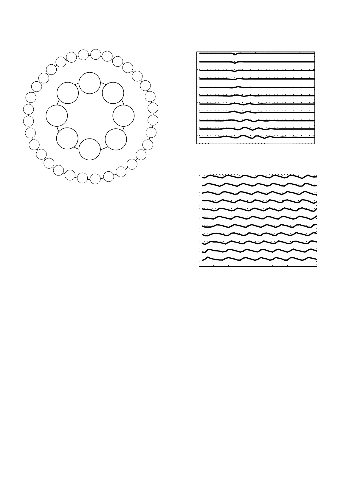
Aggressiv e shado wing of a lo w-dimensional model of atmospheric dynamics Ross M. Lieb-Lappe n a, ∗ , Christopher M. Danforth a,b,c a Department of Mathemat ics and Statist ics, Univer sity of V ermont, Burlington , VT b V ermont Advanced Computing Center , Universit y of V ermont, Burlington, VT c Comple x Systems Ce nter , Univ ersity of V ermont, Burl ington, V T Abstract Predictions of the future state of the Earth’ s atmospher e su ff er from the consequ ences of chaos: numerical weather forecast models quickly div erge fr om o bservations as uncertainty in the initial state is amplified b y nonlinearity . One measure o f the u tility o f a forecast is its shad owing time , inf ormally g iv en by th e period of time for which the forecast is a reason able description of reality . The pre sent w or k uses the Loren z ′ 96 cou pled system, a simplified nonlinear model of atmo spheric dynamics, to extend a recently developed techn ique for lengthenin g th e shadowing time of a dynam ical system. Ensemble forecasting is used to make for ecasts with and witho ut in flation , a method whereby the ensemble is regularly e xp anded artificially along dim ensions whose unce rtainty is contra cting. T he first goal of this work is to c ompare model forecasts, with and witho ut inflation, to a true trajector y created by integrating a mo dified version of the same m odel. The second goal is to establish wh ether inflatio n can increase the maximum shadowing time for a sing le optimal me mber o f the en semble. In the secon d expe riment the true trajectory is known a prio ri, an d only the closest ensem ble member s are retained at each time step, a techniqu e known as stalking . Finally , a targ eted in flation is introdu ced to both techniques to reduce the number of instances in which inflation occurs in directions likely to be incommensurate with the tru e trajectory . Results varied for inflation, with success depen dent upon the exp erimental design parameters ( e.g. size of state space, inflation amo unt). Howe ver , a more targeted inflation successfully redu ced the number of forecast degradations without significantly re ducing the numb er of forecast impr ovements. Utilized ap propr iately , inflation ha s the potential to impr ove prediction s of the future s tate o f atmospheric pheno mena, as well as other physical systems. K eywor ds: shadowing, stalking, ensemble forecasting, inflation 1. Introduction Society is ofte n depend ent u pon th e ability o f scientists to accurately for ecast the future state of chaotic physical systems, such as the weather . In extreme cases, atmo spheric scientists are asked to anticipate natural disasters with ample time for the public to ad equately prepare. T o pred ict the likeliho od of at- mospheric pheno mena, meteoro logists estimate E arth’ s future atmospher ic state using sophisticated compu ter simulations. I n general, these mathem atical models struggle to predict the spe- cific behavior of chaotic ph ysical systems due to (1) unc ertainty in the initial state, (2) chaos, and (3) mod el error [1]. The initial state is an estimate of the cond ition o f the a t- mosphere at the beginn ing o f a f orecast. Although we ather monitorin g devices o bserve m uch of the plan et, for many ar- eas ( e.g. southern hemisph ere oceans, the u pper atmosph ere) the measureme nts are spatially spar se and typ ically thr ee orders of magnitud e less in number th an the degrees of freedom in a global weather model. Theref ore, meteo rologists must c ombine observations with pr ior fo recasts to estimate initial cond itions in a process called data assimilation . ∗ Correspondi ng author Email addr esses: rlieblappen@ gmail.com (Ross M. Lieb-Lappen), chris.da nforth@uvm.edu (Christophe r M. Danforth) Since per fect knowledge of a tmospheric tenden cies is un- achiev able, a great deal of recent re search has focused on data assimilation, the proce ss by which observations are combine d with mod el prediction s to g iv e the b est possible initial state, or ana lysis [2 – 6]. It is the an alysis that is typically used as a proxy for the tru e state o f the atmo sphere at any time in the past. Althou gh the analysis has inherent uncertainty fr om lack of perfec t observations and a n impe rfect model, the modeler’ s goal is to create a forecast from th is given state that rem ains reasonable (i.e. clo se to obser vations) f or the long est d uration of time. In the context of weather prediction s, f orecasters stri ve to be accurate for two weeks, the limit imposed by ch aos. T o- day , fi ve-day forecasts are as good a s three-day forecasts were 30 years ago [7]. Despite these e ff orts, the m ischaracterization of Earth ’ s at- mospheric state in troduces un certainty . In addition , the atmo- sphere is a chaotic system , cau sing these small uncertainties in the initial st ate to grow exponentially in time. Finally , since the model itself is not a perfect representation of reality , inaccurate changes forecast by the mo del, namely model error, compoun d the un certainty and lead f orecasts to diverge qu ickly from ob- servations. As Loren z noted in 1 965, the limit of predictab ility of the atmosphere is about two weeks, e ven with nearly perfect knowledge of the curren t st ate [8]. T o accoun t for initial state uncertainty , an accepted technique Prep rint submitted to Physica D F ebruary 12, 2018 is to use ensemble forecasting , where a collection of perturba- tions to the best guess a re chosen ran domly from a distribution that reflects the measurement uncertainty and system dynamics near the given initial state [9]. Ea ch ensemb le mem ber is fore- cast forward in time, yielding a collection o f final states. Th is collection r oughly repre sents the probab ility distrib ution o f the model’ s fo recast with associated uncerta inty . For examp le, if 60% of the ensem ble mem bers predict rain, th e f orecaster as- signs a 60% chance of rain. Gi ven the limitations, the mo deler’ s goal can be stated as try ing to keep so me en semble members close to the observed truth for as long as possible, analogou s to finding a shadowing trajectory for Earth’ s atmospher e. T raditio nal ma thematical shadowing theor y was developed for hyperbo lic systems, based on the Sh adowing L emma o f Anosov [10] an d form alized by Bowen [11]. Given a pseudo- trajectory of a model (i. e. one very close to an actual one-step trajectory) , this lemm a establishes the existence of a true tra - jectory that rem ains close for an arbitrar y period of time. Later research has extended the lemma for a wide variety of hyper- bolic systems (e.g. [12 – 14]). For these systems, the nu mber of expan ding directio ns rem ains constant, i.e. the numb er of L yapunov exponents greater than zero is constan t th roug hout the state-sp ace, and small perturb ations in stable dire ctions de- cay expon entially in tim e. Ho wever , most physical systems (e.g. Earth’ s atmosph ere) are non-h yperb olic, i.e. th e num - ber of p ositiv e L yapun ov exponents fluc tuates along a trajec- tory through state space. For these systems, the re does not exist a trajectory that shadows the truth for an arbitrarily long time [15 – 17]. More recent work has been focused on finding shad- owing trajectories for lo w-dimen sional n on-hy perbo lic systems (e.g. gen eral ordinary di ff eren tial equations [18, 19], the dri ven pendu lum [20], the H ´ enon map [21]). For th e pu rposes of the present research, the time period for which a particular forecast is an a ccurate representatio n of real- ity is r eferred to as the sha dowing time . Danforth and Y orke [22] propo sed an aggressive appr oach to shadowing called stalking to increase th e shadowing time for a gi ven forecast. For a system with n -d egrees of freed om, an n -d imensional sph ere was used to enc ompass the initial ensemb le members. Throug h- out the leng th of the forecast, these members experience expan - sion away from each other in some dimensions and contraction tow ard s each other in others, dependin g on the local finite-time L yapunov exponen t in eac h d imension. Th e en semble forecast can be appr oximated by a n n -dimen sional ellipsoid f or a short time. The idea of stalkin g is to artificially impose some additional uncertainty in th e co ntracting d irections (i. e. tho se with a neg- ativ e local finite-time L yapunov exponen t) at period ic inter- vals throu ghout the f orecast. This is a ccomplished by inflating the ellipsoid along axes parallel to the contracting dimensions. Thus, if the true state o f the system happens to suddenly expand along a previously contractin g direction, as happens in systems exhibiting un stable dimension variability [23], some e nsemble members will r emain relatively close to the true state. Stalking is no t curr ently used in weather fo recasting, but an alternative version called variance infl ation is u sed in ensem ble-based da ta assimilation to e nsure the state estimation alg orithm d oes not put too much faith in the mo del forecasts and ign ore observa- tions when creating the analysis [24]. For the purp ose of this paper, th e te rms “shadowing” an d “stalking” are re served f or experiments where the truth is known a prior i, and the goal is to id entify an optimal ensem- ble member (section V). Using the technique de scribed above to create forecasts, without prior knowledge of the tru th, is h ere denoted forecasting with and without inflation (section IV). In section II , we presen t the n on-h yperbo lic ’96 Lo renz system [25] and the mo del, and examine the e ff e ct o f chang ing b asic parameters. I n section III, the process of creating the initial en- semble and m aking forecasts is explain ed. In section IV , the inflation techn ique is in troduc ed, and fo recasting results ( with and without inflation) are presen ted. In section V , we present the results from s talkin g experiments. In section VI, we use tar- geted inflation to isolate the instances in which inflation is mo st likely to im prove a forecast. Finally , the finding s are discussed with respect to operatio nal weather prediction in section VII. 2. The Lorenz 1996 System In num erical weath er p rediction ( NWP), the tru e evolution of the Earth’ s atmospher e will ideally be a plausible m ember of an en semble forecast [9]. In our context, ensemble forec asting is used to model the trajectory z a , th e “truth , ” of some meteo - rological quantity (e.g. tempera ture, pressure). In the present study , both the truth an d th e forecast were c reated using ver- sions of a simplified n onlinear model giv en by Lorenz (1996 ) to re present the atmo spheric behavior at I equ ally spaced loca- tions on a given latitude circle [25]. T his system has be en used to represent weather related dynamics in many previous s tud ies (e.g. [26 – 2 8]). Th e governing first-order di ff er ential equatio ns are giv en by [25]: d x i d t = x i − 1 ( x i + 1 − x i − 2 ) − x i + F − hc b i J X j = J ( i − 1) + 1 y j , (1a) d y j d t = − cby j + 1 ( y j + 2 − y j − 1 ) − cy j + hc b x floor[( j − 1) / J ] + 1 (1b) for i = 1 , 2 , . . . , I , j = 1 , 2 , . . . , J I , and n = ( J + 1) I . Altho ugh n represents the full state space size, we are prim arily interested in the values of the slow v ariab les x i . Thu s, for the pur poses of this study we consider I to be the dimensionality of the system. The values x i represent slowly ch anging meteorolog ical quantities whose dynamics are described by Eq. (1a ). Since the set o f x i correspo nds to locations along a single latitude circle, the subscripts i and j are defined to be in a c yclic chain. That is, we defin e x − 1 = x I − 1 , x 0 = x I , and x 1 = x I + 1 , and similarly for j . Each x i is th en coupled to J quickly changing, small ampli- tude v aria bles whose beha v ior i s g overned by Eq. (1b). For our experiments, we set I = 4 , 5 , 6 and J = 16 yielding n = 68 , 85 , 2                                                                                         Figure 1: Model Schematic [26 ]. T he I = 8 slow va riables x i can be thought of as locati ons al ong a latitude circle. E ach varia ble has J = 4 corresponding y j fast v ariables for a total of n = 40 degr ees of freedom. and 102 variables. A schematic is shown in Fig. 1 where eight slow v ariab les ( x i ) are each cou pled to four fast variables ( y j ), reflecting a total of n = 40 degrees of fr eedom. No te th at the dynamics of each x i are dictated by neighbo ring x v ariables and the corr espondin g set of cou pled y j variables. As a low-dimensional model of atmo spheric dynam ics, th is system is ideal for several reasons; p rimary among them being the ability to tune the relati ve levels of nonlinearity , coupling of timescales, and spatial degrees of fr eedom. The no nlinear terms in Eq. ( 1a) are mean t to represent advection, an d conserve the total energy of the system . Th e lin ear term signifies a loss of energy either throug h mech anical or th ermal dissipation . E x- ternal forcing F is then adde d to p revent the total energy from decaying co mpletely . For all experiments we set F = 14 . Con- sistent with the literatu re, we set c = 10 and b = 10, wh ich forces the fast variables to oscillate 10 time s quicker than the slow variables [ 17, 26, 28]. The coupling parameter is set to a value of h = 1 for th e system truth, and h = 0 . 5 for the model. Note that one time unit correspon ds to five d ays, the dissipative decay time [29]. Integration of the di ff eren tial equations is completed u sing the fourth order Rung e-Kutta meth od with a time step o f 0 . 01. Rigorous shadowing attempts co uld be made using far mor e advanced method s of integration, with much s ma ller time steps [30]. Howe ver, for the pur pose of this study of short forecasts, the di ff eren ce is negligible . 2.1. Dynamics The sy stem dynamics can be obser ved b y integratin g Eqs. (1a) and (1b) with h = 1, he reafter referred to as the sys- tem . In Fig. 2, a tim e series fo r a particu lar lon gitudinal pro- file ( I = 40 , J = 1 6) is shown after variable x 13 is initially 0 5 10 15 20 25 30 35 40 0 1 2 3 4 5 Site Time (days) 0 5 10 15 20 25 30 35 40 0 1 2 3 4 5 (a) Days 0 − 5 0 5 10 15 20 25 30 35 40 50 51 52 53 54 55 Site Time (days) 0 5 10 15 20 25 30 35 40 50 51 52 53 54 55 (b) Days 50 − 55 Figure 2: A time series of the system sho ws t he e ff ect of a fiv e-unit p erturbation. Pane l (a) shows days 0 − 5 and panel (b) shows days 50 − 55. Perturbati ons appear to mo ve pr imarily to the east (r ight). After fi ve days, pertu rbation e ff ects can be observ ed at over half of all the loc ations ( I = 40 , J = 16). perturb ed by five u nits. Profiles are r ecorded at 1 2-h inter vals for day s 0 − 5 (pane l a) an d da ys 50 − 55 (pan el b). Advec- tion is apparent as the energy f rom the perturbatio n is observed halfway arou nd the latitudin al circle by d ay five. L orenz and Emanuel [ 29] calculated a p erturb ation g rowth rate (dou bling time) of appro ximately two days for this mod el, which agrees with trends in larger atmospheric models where er rors doub le in rou ghly two da ys [31]. However , growth rates over limited time intervals as in Fig. 2(b) can di ff er greatly depen ding on I and J . Adjusting the par ameters of the system, an d examining the time series at a sin gle latitudinal site, the inter depend ence of the slo w and fast variable coup ling is observed. For examp le, with I = 6 and J = 16, a “regular” oscillatory pattern occurs as an energy equilibriu m is achieved between e xter nal forcing and dissipation. In this work , we will use the term “regular” to refer to these q uasi-perio dic patterns. Howe ver, as the significanc e 3 of the fast variables is reduced b y lowering the coupling par am- eter h , the time series bec omes more co mplex. Less en ergy is able to dissipate from slo w variables to fast, leadin g to greater irregularity in x i . Similarly , the regularity of a time series can be a djusted by varying the numb er of slow or fast variables. As illustrated in Fig. 3 (acr oss co lumns), increasing J creates a more r egular system for all values of I . For I = 6, the system is fairly re gu lar for both J = 16 and J = 40. Howe ver , with only a few fast variables acti ve (e.g. J = 8), o scillations become increasing ly aperiodic. For I = 8, ad ditional fast variables are requir ed to achieve the consistent pattern; they allow the system’ s en ergy to be mo re evenly distributed, an d no nlinearities in the fast v ari- ables have less impact on the stability of the slow variables. Adjusting the numb er of slow v ariab les gr eatly alters the qualitative dynam ics o f the time series fo r each p articular x i (Fig. 3, across rows). For J = 8, only I = 4 exhib its regularity . Howe ver , with additional fast v ariab les ( J = 16), the I = 6 sys- tem e x hibits the greatest regularity . For I = 4, the slow variable relativ e maxima are more pronounced th an the relati ve m inima, and the system ap pears to be q uasi-period ic with a domin ant frequen cy of roughly ten d ays. For I = 6, the symmetr ical pat- tern em erges with a frequ ency of r ough ly five da ys. This pattern is similar when J is increased to 40, b ut with decr eased ampli- tude. However , for I = 4 and I = 8 with J = 40, the p attern being repeate d is more complex. W e make the precedin g observations to mo tiv ate the cho ice of Lorenz ’9 6 as an app ropriate testbed with which to perf orm ensemble forecasting exp eriments. The d ynamics a re quite sen - siti ve to the system parameter s, and we will describe fore cast results, which vary depending on the underlying dynamics. 2.2. Coupling Each x i in the system is cou pled to J small-amp litude fast variables y j , and the strength of this couplin g is controlled b y the param eter h . As m entioned above, the system is d efined by setting h = 1 . Howe ver , th e model is r endered imperfec t by dampen ing the e ff ect of the fast v ariab les in Eq. (1b) by setting h = 0 . 5 , her eafter referred to as the mo del . A 20 day time se- ries for a single x i with its correspon ding y j ’ s is sho wn in Fig. 4 ( I = 8 , J = 4). In the top f rame we compar e th e time series of x 1 for integration s o f the same initial c ondition b y both the system and the mod el. By day 2 0 th e x 1 values di ff er b y the climatological span of x 1 . In a ddition to increasing the amp li- tude of slo w variable oscillations, reducing the cou pling h has the e ff ec t of c reating a less r egular time series. Note that th e fast variables ( shown for the system) vary with am plitudes o n the ord er of 10% of the slow v ariables. 3. Methods From a given initial condition, the trajectory of the truth ( z a ) is cr eated by integrating the system in Eqs.(1a) and (1 b). T wo- and three-dimension al vie ws of orbit segments of this attractor with I = 4 , J = 16 are shown in Fig . 5 (a) an d 5 (b). As men- tioned above, the foreca st for eac h ensemble memb er is then −15 0 15 X 1 −2 0 2 y 1 −2 0 2 y 2 −2 0 2 y 3 0 5 10 15 20 −2 0 2 y 4 Time (days) Figure 4: A 20 day time seri es for x 1 and y 1 , 2 , 3 , 4 using I = 8 , J = 4. For the top frame, the solid line represents the time series for x 1 with fast vari able couplin g set at h = 1 (the system). The dashed line has fast var iable coupling reduced to h = 0 . 5 (the model). T he bottom four frames are the fast va riable time series for the system y 1 , 2 , 3 , 4 coupled to x 1 , as illustr ated in Fig. 1 created by reducing the weight of th e fast v ariab les by 50% in the model, relative to the system. T w o- and thr ee-dimen sional slices for the model can be seen in Fig. 5 (c) and 5(d ). Th is particular experimen tal design was cho sen as it is typica l f or global atm ospheric mod els to attem pt to parameterize sub-grid scale behavior (e.g. for phenomen a o ccurrin g on a finer tempo- ral / spatial scale). 3.1. Ensemble cr eatio n The experimen tal d esign is inspired by and fo llows that of W ilks [26]. First, long integrations o f the system on random - ized in itial values were perform ed to estab lish the shape o f the attractor . A set of 5 00 di ff eren t I -dimension al points were then chosen at 250-day intervals. This spacing was chosen to ensure that the initial states sampled di ff eren t regions of the system attractor, an d neighb oring states were un correlated . A ‘tru e’ trajectory z a from each of these states was dete rmined using a 50-day integration of the system. T he goal is to use the model to shad ow each of these in dividual true trajectories with an en- semble of 20 members. Care was taken to establish an en semble that was a dynamically realistic sample of state space near the initial state as follows. At each of the 500 in itial states, an I -d imensional hy per- sphere was c onstructed e ncompa ssing 10 0 neigh boring states from the system attracto r , identified during a very long system integration. A neighb oring state is defined to be one within 5% of the span of x i in the i th dimension of the attractor . For each hypersp here, the cov arian ce of th e 100 neighbor ing states is cal- culated, yielding a I × I matrix C . The matrix values are then scaled to ensure t h at the average ensemble standard deviation is 5% of the climatological span of the system attractor . Thus, for each of the 500 h ypersph eres, 20 initial ensemb le members are drawn from the distrib ution : 4 0 10 20 30 40 50 −10 −5 0 5 10 15 Time (days) X 3 (a) I = 4 , J = 8 0 10 20 30 40 50 −10 −5 0 5 10 15 Time (days) X 3 (b) I = 4 , J = 16 0 10 20 30 40 50 −10 −5 0 5 10 15 Time (days) X 3 (c) I = 4 , J = 40 0 10 20 30 40 50 −10 −5 0 5 10 15 Time (days) X 3 (d) I = 6 , J = 8 0 10 20 30 40 50 −10 −5 0 5 10 15 Time (days) X 3 (e) I = 6 , J = 16 0 10 20 30 40 50 −10 −5 0 5 10 15 Time (days) X 3 (f) I = 6 , J = 40 0 10 20 30 40 50 −10 −5 0 5 10 15 Time (days) X 3 (g) I = 8 , J = 8 0 10 20 30 40 50 −10 −5 0 5 10 15 Time (days) X 3 (h) I = 8 , J = 16 0 10 20 30 40 50 −10 −5 0 5 10 15 Time (days) X 3 (i) I = 8 , J = 40 Figure 3: A 50 d ay time series for x 3 illustra tes the depende nce of the syst em stabil ity on the n umber of slow ( I ) and fast ( J ) vari ables. The number of slow v ariables v aries from I = 4 (a-c) to I = 6 (d-f) to I = 8 (g-i). The fast v ariable s vary from J = 8 (left column) to J = 16 (mid dle column) to J = 40 (right column). Generally , increa sing J leads to increased regular ity , while changes in I have an impac t that is dependent upon the magnitude of J . 5 −5 0 5 10 15 −10 −5 0 5 10 15 X 1 X 3 (a) T wo-dimensi onal vie w of orbit segment of system attrac tor −5 0 5 10 15 −5 0 5 10 15 −5 0 5 10 15 X 1 X 2 X 4 (b) Three-dimension al vie w of orbit segment of system attra ctor −5 0 5 10 15 −10 −5 0 5 10 15 X 1 X 3 (c) T wo-di mensional view of model attrac tor −5 0 5 10 15 −5 0 5 10 15 −5 0 5 10 15 X 1 X 2 X 4 (d) Three-dime nsional vie w of model attrac tor Figure 5: System (a-b) and m odel (c-d) attrac tor . Panel s (a ) and (c) show two-dimensi onal vie ws looking at x 1 vs x 3 . Panels (b) and (d) show three-dimensio nal vie ws using x 1 , x 2 , and x 4 ( I = 4 , J = 16). 6 C init = 0 . 05 2 τ 2 λ C , (2) where λ is the average eigen value of C a nd τ is the stand ard deviation of x i observed in the attractor . First, a contro l state is picked within e ach h ypersph ere b y adding appropr iately distributed rando m noise to the I slow variables of the truth as follo ws: z f 0 ( i , 1) = z a 0 ( i , 1) + p C init y ( i , 1) , (3) for i = 1 , 2 , . . . , I . The vector y is I -d imensional, consisting of random entries from a Gau ssian distrib utio n. The Cholesky decomp osition is used to calc ulate the squ are roo t of C init [32]. Note that if C init was n ot symm etric p ositiv e definite ( due to the fin ite sample in time) , then the lower triang ular matrix was matched to the upper tr iangular matrix. The remainin g 19 en- semble memb ers a re the n chosen using the sam e meth od, but using th e co ntrol state z f 0 ( i , 1) for i = 1 , 2 , . . . , I as the central referenc e point. Thus, we hav e z f 0 ( i , m ) = z f 0 ( i , 1) + p C init y ( i , 1 ) , (4) for i = 1 , 2 , . . . , I and m = 2 , 3 , . . . , 20, wh ere z f 0 is a m atrix with ensemb le members as colum ns. Finally , the initial fast variables for the forecast are set equ al to the in itial fast variables of the truth, z f 0 ( j , m ) = z a 0 ( j , 1) for j = I + 1 , I + 2 , . . . , I ( j + 1) a nd m = 1 , 2 , . . . , 20. These fast variables are subsequently ignored when measuring the shadowing time. 3.2. Characterizing the ensemble Once the en semble of initial states has been created f or each hypersp here, the trajector y of each ensemble member is fore- cast using the model. Let A be the I × ( m − 1) matrix of ensem- ble memb ers with the control state at the origin, where m is the number o f ensemble memb ers (inclu ding the control fo recast) and we are only considering slo w variables. If the matrix A acts on every vector in the ( m − 1)-d imensional u nit spher e, the result is a filled-in ellipso id, provide d m > I . Th e p oints within the ellipsoid can be thoug ht of as rep resenting all pote ntial ensem- ble members based upon the known m m embers (all of wh ich lie within this elli p soid). Althou gh the system is chaotic, ov er a short time span one can approximate the nonlinear e volution of the initial sphere of trajector ies with this ellipsoid [33]. Every two time steps, the e llipsoid is analyzed to de ter- mine expandin g and con tracting directions (i.e. those direc - tions with positive / negati ve local finite-tim e L yapunov expo- nents). This frequ ency was chosen rather than every time step to ensure the identified directions continue to e xp and / co ntract. Let A = U S V ⊤ be a singular value deco mposition (SVD) o f A , and let s ( t ) = s 1 , s 2 , · · · , s I be the singular values (the di- agonal entries of S ) and U ( t ) = [ u 1 , u 2 , · · · , u n ] th e matrix of left-singular vectors at a giv en time t . T hus the lengths an d di- rections of the semi- axes of the ellipsoid appro ximately enc om- passing all poten tial ensemble m embers ar e given by s i u i [32]. At ea ch time inte rval, th e vector s ( t ) is compare d to s ( t − 1) −5 0 5 10 15 −5 0 5 10 X 1 X 2 s 2 u 2 s 1 u 1 Figure 6: A two- dimensional represent ation of a 20-member ensemble ( I = 2). The black poi nt is the control forecast, and the white points are the othe r ensemble members. Let A be the 2 × 19 matrix of ensemble members with the control forec ast defined as the ori gin. The semi-axe s are calculat ed using SVD, where s 1 and s 2 are the two sin gular value s of the matrix A . Note that the SVD spectrum can be quite steep for forecasts longer than a fe w time steps. (the sing ular values from th e previous time in terval) to deter- mine which singular values ar e d ecreasing. W e then computed the do t p rodu ct b etween all p ossible com binations of f ormer u i ( t − 1) and current u i ( t ) left singular vectors, with the largest dot pro duct chosen to identify direction pa irs. Note that on oc - casion, a perf ect matching was not achieved, but t h e best guess was used. A two-dimen sional analo g is shown in Fig. 6 . Note all en semble m embers lie within th e ellipse, and the contr ol state is located at the center by definitio n of A. SVD allows us to identify the ellipse semi-axes s 1 u 1 and s 2 u 2 . An example one-d imensional 4 0 day ensemb le f orecast is shown in Fig. 7 ( I = 6 , J = 16 ). No te th at for the first 20 days, almost all ensemble memb ers remain close to th e tru th. Howe ver , by day 4 0 the spread of ensemble mem bers covers th e entire state space, and the ensemb le mean no long er accurately represents the truth. In addition, Fig . 7 illustrates tha t th e model achieves greater extreme values than the system. With less en- ergy being dissipated th rough the fast variables, more energy remains oscillating between the slow variables in the mod el, as compare d to the system. Note that the reduced re gu larity of the model relativ e to the system can also be observed. 4. Forecasting Forecasting often fails when the state sp ace d ynamics of the physical system expand alo ng a p reviously contra cting dimen- sion. A tw o -dimension al illustration of th is concept is s hown in Fig. 8. Because of the uncertainty associated with the initial lo- cation of the truth, an I -d imensional sphere o f radiu s σ is used to rep resent the tru th. It is from within this sph ere that th e initial ensemble members a re chosen. Th e ellipse representin g the en- semble members div erges from the trajectory of the truth when the system quick ly turn s in a ne w direction. In the illustration, 7 0 5 10 15 20 25 30 35 40 −10 −5 0 5 10 15 Time (days) X 3 Figure 7: A 20-member ensemble forecast for x 3 initia lized using Eq. (4) . The black line represents the truth, an integra tion of the system. The gray lines are indi vidual ensemble members, integra tions of the model ( I = 6 , J = 16). σ z Z 1 f Z 2 f 0 a z F a 3 = Z Z f f F Figure 8: Schematic of forecasting in two dimensions. The black line rep- resents the tra jectory of th e truth ( z a ). Z f t is the ell ipsoid encompassing the ensemble members at time t , and the da shed line is the trajec tory of the ensem- ble mean. For nonlinear systems, this ellipsoid is only a good ap proximation of the collectio ns of forecasts for s mall t . Note that the time steps 0 , 1 , 2 , 3 are an incomplete sampl ing of all time steps. The goal of a forecast is to achie ve an ensemble which has a n onempty intersectio n with z a F . Here forecasti ng fails after time 2. forecasting has failed at tim e F as there is no overlap between the I -d imensional sph ere aroun d th e truth z a F and th e ensem - ble ellipsoid Z f F . For all experiments, the number of expanding directions observed thr ough out the f orecast was non -constant. This u nstable d imension variability is a cause of shadowing failures well-documen ted i n the literatur e [22, 23, 34, 35]. 4.1. F orecasting with inflation As de scribed in th e intro duction , inflation is perfor med in an attempt to improve the en semble forecast by expanding th e ellipsoid along contracting d imensions of the state space. For each direction u i in wh ich th e en semble is contractin g, ensem- ble member s are inflated along th e i th semi-minor axis of the ellipsoid s i u i . Althou gh this add s ar tificial unce rtainty to the forecast, Danforth and Y orke argue that th e amo unt is minimal [22]. If th e ellipsoid continues to co ntract in these dimension s, the synthetic unce rtainty co ntinuo usly decreases. However , if φ - inflation σ z 0 a Z 1 f Z 2 f 3 = Z Z f f F z F a Figure 9: Schematic of foreca sting with inflation in tw o dimensions. The black line represents the traject ory of the truth. Z f t is the ellipsoid encompassing the ensemble members at time t , an d the dashed line is the tr ajectory of the ensem- ble mea n. At each time step, the ellip soid is inflated by ϕ along co ntracting direct ions, where in this case there is only one such direction. Note that fore- casting no w achie ves its goal in contrast to F ig. 8. the system begins to expand along a pr eviously contractin g di- mension, the inflated en semble will capture some o f the change. This concept is illustrated for two dimensions in Fig. 9. As described above, the d irections of the sem i-axes a re cal- culated using SVD througho ut the fo recast at period ic time in- tervals an d s ( t ) is compare d to s ( t − 1 ). For each i in which s i < s i ( t − 1), all ensemb le m embers are in flated in direction u i . I t is impor tant to note here that if inflation were per formed in expanding dimensions as well, forecasts would degrade mor e rapidly . By co nstraining inflation to the co ntracting d imensions, we are min imizing the dam age caused in hy perbolic regions of state space. Let ϕ be the inflation amount, expressed as a p ercentage o f the semi-axis length, and let A be the matrix of ensemble mem- bers with the contr ol state at the or igin, p rior to inflation. Define M = I + ϕ ( u i u ⊤ i ) (5) where I is th e I -dimen sional ide ntity matr ix, u ⊤ i is the transpose of u i , an d let A ′ = M A . Add ing the con trol state to each vector in A ′ then yields ensemble membe rs inflated by ϕ in direction u i . The benefit of inflation f or a particular forecast is illustrated in Fig. 10 for a two-d imensional projectio n of a n ensem ble fore- cast ( I = 6). As the tr ajectory of z a begins to tu rn clockw ise, the forecasts (gray lines) diverge fr om the black line. As repr e- sented by th e gray lines, f orecasting fails at location 1 without inflation (Fig. 10a), wh en there is no longer overlap between the σ -sphere sur round ing z a and the ensemble ellipsoid. Howev er, in Fig. 10b, the g ray line s are in flated at locatio n 1 in pre viou sly contracting directions (as inferre d fr om SVD of the model en- semble). Note t h at th e gaps in the figu re represent b oth an in fla- tion and a time step. As the figure illustrates, these shifts help capture the change in d irection fo r z a . It is imp ortant to note that no measurements of z a are used to determine th e directions in which to inflate. A second inflation fo r the gray lines oc- curs f our time steps late r at location 2 in panel b. At first there is m ore unc ertainty in the ellipsoid enco mpassing the ensem- ble member s. Howe ver , as z a continues in the sam e direction, the uncertainty is dampened by the contracting dynamics. Note 8 7 7.5 8 −2 0 2 4 X 2 X 3 (a) No inflation 7 7.5 8 −2 0 2 4 Inflation 1 Inflation 2 X 2 X 3 (b) Using inflation Figure 10: Successful inflation in an ensemble forecast. T he black line is the true t rajectory z a , and the g ray lines a re ensemble member fore casts without in- flation (panel a) and with inflatio n having the potential to occur at a minimum of e very tw o time steps (pane l b). All traj ectories are movi ng in a clo ckwise di- rectio n. At locati on 1, forecasting fail s without inflation. Location 2 represents a second i nflation of the e nsemble. Inflation suc cessfully modifies the ensemble to include the truth as a plausible m ember . Note that no observat ions of z a are used during the inflation at locati ons 1 and 2 ( I = 6 , J = 16). that although the ellipsoid is analyzed e very two time steps, the model did not inflate between locations 1 and 2. Also, inflation acts symmetrically on an ensemble, lea ving the ensemble mean unchan ged during a single step. Ho wever , once the ensemble is integrated forward in time, the inflated and n on-in flated ensem- ble mean forecasts diver ge . 4.2. Results For each of th e 500 initial hyperspher es, a 5 0-day mod el for e- cast fo r the 2 0 ensemble mem bers was created with and with- out inflation. At each poin t in time, let z ∗ be the m ean of the 20 ensemble mem bers’ slow variables. For each hy perspher e, z ∗ was compare d to the slow variables of the truth , wher e we let z a represent only the slow v aria bles for simplicity . The r oot mean square error (RMSE) and anomaly correlation (A C) were calculated at each time step as follows: R M S E = k z ∗ − z a k 2 (6) AC = ( z ∗ − z ) · ( z a − z ) k z ∗ − z k 2 k z a − z k 2 (7) where z represents the vector of system clim atological av er ages for each slow v ariable . RMSE and AC calculations were then av erag ed over all hypersph eres for the dura tion of each f orecast. For the system, RMSE ≈ 9 represents satur ation, at which p oint there is no similarity between the forecast and the truth. For the p resent discussion, we consider the period for wh ich a forecast is useful, namely the time for which A C remains above 0 . 6 [7]. For each state space size, the average u seful time was calculated using th e non -inflated forecasts. This y ielded du - rations o f 6 . 7 , 8 . 7 , and 17 . 0 days, c orrespon ding to I = 4 , 5 , and 6 , respe ctiv ely . If the inflated and non-in flated f orecasts crossed the 0 . 6 th reshold d uring the same time step, the u seful times were con sidered indistinguishab le. Inflatio n was deemed to h av e “su cceeded” if the du ration for a n acceptab le fore- cast improved by mo re than 5% of the a verage useful time for ϕ = 0 forecasts. Similarly , th e technique was co nsidered to have “failed” if the dura tion worsened by the same th reshold. If there was any improvement (greater than one time step) with inflation, forecasts were denoted “in flation helped . ” Any mea- surable degradation with inflation w as labeled “inflation hurt. ” Results for I = 4 , 5 , and 6, with ϕ = 0 . 5 % , 1% , 2% , an d 5%, are r ecorded in Fig. 11 with totals ou t of 500. Bars above zero represent improvements, while bars below z ero repre sent degra- dations. Black bars indicate improvements and degradation s of more than 5% o f the average useful tim e (i.e. the n umber of successes and failures) . Other metrics such a s RMSE an d the trajectory of the best ensemb le mem ber were conside red, but they showed the same ge neral trend s. For all experim ents de- scribed by Fig. 11, J = 16 as illustrated in Fig. 3. Although th e sample size is small, Fig. 11 suggests that infla- tion has a greater e ff ect for larger I , with the b est results e xh ib- ited for I = 6 an d ϕ = 1%. In fact, the num ber of hyper spheres in which inflation helped was an orde r o f magnitude b etter for I = 5 than for I = 4. The vast majority of inflated I = 4 fore - casts were iden tical to no n-inflated ( ϕ = 0) f orecasts. These number s roughly doubled for I = 6 relativ e to I = 5, likely due to the incre ased regularity in z a for I = 6 ob served in Fig. 3. Unfortu nately , the same trend is seen for forecasts in which in- flation failed. By capturin g one of th e sudd en changes in the trajectory of the truth using inflation, the model can better fore- cast the tru th fo r a long er dur ation. Alternatively , this incr ease in the occurrence of inflation helping might be e vid ence th at er - ror introduced b y inflation in contractin g directio ns has a min- imal e ff ect, as argued by Danforth and Y orke [22]. This e ff ect would likely be strongest in systems wit h a steep singular value spectrum, where the expanding dimen sions p lay a m ore domi- nant role. Naturally , the success of inflation is also strong ly dep endent on ϕ , with increasing ϕ gen erally co rrespon ding to a larger 9 0.5 1 2 5 0.5 1 2 5 0.5 1 2 5 −200 −100 0 100 200 300 400 φ I=4 I=5 I=6 Number of Hyperspheres Figure 11: Inflati on forecasting results for 500 hyperspheres. Bars abov e zero sho w the number of hypersph eres for which inflation improv ed the foreca st, while bars belo w zero show the number of hypersphere s for which inflation degra ded the forecasts. Black bars indicate improvement s and degradati ons of the a verage shado wing time b y more than 5% (“ inflation succee ded” and “in fla- tion fail ed, ” respecti vel y). Gray ba rs represent the cat egories “inflation helped” and “i nflation hurt. ” The number of times infla tion impro ved the forecast g ener- ally exceede d the number of degrada tions, both of which tend to increase with dimensiona lity and ϕ . number of both successes and failures. By increasing the in - flation amount, the ellipsoid encompassing the ensemble mem- bers is m ore likely to overlap with the tr ajectory of th e truth, and thus capture unstable dimension variability events. On the other hand, in flation can make a forecast worse. By inflating in di- rections incommensurate with th e tru th, the method intr oduces additional error , which can be quite significant when amplified by nonlinearity . The numb er of hypersphe res in which i n flation failed also n aturally incre ases with ϕ . Howe ver , as m entioned above, provided the contracting directions continue t o contract, the erro r introduced is hopefully minimal. For a gi ven set of experimental param eters, the a veraged u se- ful time over all 500 h ypersph eres is used fo r analy sis. How- ev er, the ϕ = 0 f orecast provid es an ind ividual u seful time for each hype rsphere. Whether or not inflation helps or hurts (i.e. reduces or increases the individual useful time) is no t d ependen t upon the magnitude of the individual useful time. For example, inflation is eq ually likely to help (or hurt) an ind ividual forecast whose non-in flated useful time w as 3 d ays or 20 days. As shown in Fig. 11, for m any o f the hyper spheres infla- tion successfully im proved the d uration f or which a forecast is useful. The lack of harm cau sed by this tech nique in a g lobal sense can be seen by averaging RMSE and A C over the hy per- spheres in which inflation was successful as shown in Fig. 12 for I = 6 , J = 16 . Both plots sh ow small improvement rel- ativ e to forecasts ma de with no inflation . I n section VI, we demonstra te the ability to isolate c ondition s likely to resu lt in successful inflation as in Fig. 10. Conducting exper iments for larger dimension al systems was di ffi cult due to com putation time limitation s fo r estimating the local dynam ics of th e system attractor (see Section III). T o re- 0 5 10 15 20 25 30 35 0 3 6 9 12 15 Time (days) RMSE All Trajectories 0 5 10 15 20 25 30 35 0 3 6 9 12 15 Improved Trajectories (a) RMSE 0 5 10 15 20 25 30 35 0 0.2 0.4 0.6 0.8 1 Time (days) AC All Trajectories 0 5 10 15 20 25 30 35 0 0.2 0.4 0.6 0.8 1 Improved Trajectories (b) A C Figure 12: A ve raged RMSE (a) and A C (b) for the I = 6 , J = 16 system. The dashed line repr esents no inflati on, while the solid line is with infla tion of 1%. Figures sho w the average d data for all 500 hyperspheres, while insets only include the hyperspheres for which inflation succeeded. Giv en the small (positi ve) change in avera ge forecast statistic s, the method is unlikel y to harm forecast s, and may be adjusted to isolate parti cular e vents for which inflation can be quite successful (see Section VI). duce the computatio nal b ur den, initial ensemble members were chosen using a spherically -symmetric Mo nte Carlo appr oach (i.e. n earby initial conditions but with n o attracto r-imposed structure) for these larger systems ( I = 7 , 8 , . . . , 40) . The I = 6 , I = 16 , and I = 2 1 sy stems had substantially greater a v- erage usefu l times than the other systems (b y a factor of five). These specific system s all exhib it increased regularity in their time series ( see Fig. 3), presumably a result of some r esonance between th e slow an d fast variables. For these systems th e model is most sensitive to inflation , with small ϕ grea tly im- proving forecasts and larger ϕ g reatly degrading forecasts. The less-regular systems had smaller incid ence of success and fail- ure, with results similar to tho se observed for the I = 4 and I = 5 systems. Howe ver, the use of a spherically -symmetric 10 −5 0 5 10 15 −5 0 5 10 X 1 X 2 Figure 13: Schematic of th e redefining of a shad owing ensembl e in two dimen- sions. The star represents the known locati on of the truth. The solid circl es are supplement ed by a coll ection of point s m eant to approximate the ov erlap of th e ellip se and the sphe re around the truth. The open c ircles are pre vious ensemble members that will now be redefined within the overla p, which is approximat ed by a new el lipsoid. Note tha t the x 1 , x 2 axe s are exagge rated for visual ease. Monte Carlo appro ach to initialize an ensemble degraded the perfor mance of inflation when compared to the more soph isti- cated ensemble initialization techniqu e. 5. Shadowing and Stalking 5.1. Methods Shadowing with an ensemb le presents an alter native method for assessing the quality of a mo del’ s predictions. Contrasting the forecastin g experiments describe d previously , in this co n- text the trajectory of the tru th is kno wn a priori to within a gi ven uncertainty ( σ ), an d its lo cation at a given time is rep resented by an I - dimensiona l sphere o f rad ius σ . At regular intervals, the intersection between the ellipsoid enco mpassing the ensemble members and the σ -sphere is approximated . The ensemble el- lipsoid is th en red efined to represent the in tersection, while the other ensemble me mbers are redefined to fall with in the over- lap. Provid ed this intersectio n is n onemp ty , the trajectories of some ensemb le m embers yield accu rate representation s of re- ality . A schematic of this techniqu e is shown in Fig. 13. Note that althoug h the actual truth lies outside th e ensemb le ellip- soid, som e ensem ble memb ers are with in σ . The trajectorie s of these ensemble memb ers can b e forecast f orward in time, and the process is repeated. If some ensemble members remain in the intersection for the entire for ecast, then their trajec tories have successfully σ -shadowed the truth. When inflation is ap- plied to the ensemb le ellipsoid (as described previously), this aggressive form of shadowing is called stalking . 5.2. Results The same initial cond itions utilized in the for ecasting exper - iments wer e used to create 50 -day stalking en sembles. Ho w- ev er, every four time steps the ensemb le ellip soid was r edefined 0.5 1 2 5 0.5 1 2 5 0.5 1 2 5 −100 −50 0 50 100 φ I=4 I=5 I=6 Number of Hyperspheres Figure 14: Stalking results for 500 hyperspheres. Bar categori es are identical to those in Fig. 11. Inflation improves and worsens the abilit y to shado w with similar probabilit y . Counts tend to s lightl y increase with the dimension of the system. as described in Fig. 13. This fr equency was cho sen to b e long enoug h to ensure that appropriate con tracting dimensions could be identified. During the definition o f the overlap between the ensemble ellipsoid and the truth sphere, semi-axes can b e al- tered drastically , requiring se veral time steps to reflect the local dynamics. The σ -sh adowing distance (un certainty aroun d the truth) was chosen to b e 10% of the climatolog ical rang e in each dimension, name ly twice the spr ead in the initial en semble. A new collection of 20 ensem ble member s were then chosen ly- ing within th e red efined ellipsoid. As befor e, RMSE an d A C were calculated an d comp ared fo r both shad owing and stalk- ing exper iments. Cou nts for the n umber of hyper spheres for which inflation succeeded , failed, helped, and hurt as described in Section IV were tallied. Results for I = 4 , 5 , an d 6, with ϕ = 0 . 5 % , 1% , 2% , and 5%, are given in Fig. 14. The shadowing experimen ts exhibited a greater benefit from inflation when the dimensionality I is large, although the di ff er- ence is less than be fore. Howe ver, th e nu mber of hyperspheres for which inflation succe eded doe s not seem to trend mon o- tonically with ϕ over the range 0 . 5% − 5%. Since the num ber of hy persphe res in which inflation succeede d rough ly eq uals the numb er fo r whic h inflation help ed, we can con clude that when stalkin g is con structive, it improves the shadowing time by mor e th an one day . On the other han d, the nu mber of hy- perspher es in wh ich in flation succeeded is nearly equivalent to the number for which inflation fail ed for all experiments. Thus, inflation can also have a negati ve e ff ect upon s ha dowing. As with fo recasting, stalking experim ents were extended to higher d imensional system s u sing a spherically- symmetric Monte Carlo appro ach for ensemble initialization. Similar to the lower dimen sional system s in Fig. 14, counts for the num ber of hype rspheres fo r which inflation succeed ed and failed were relativ ely close. For small values of inflation, there were often errors in the pr ocedur e by which cor respond ing ensemb le semi- axes dire ctions are calculated between time steps, resulting in 11 an in crease in the num ber of failures. With larger inflation, the algorithm can b etter determine co rrespon ding direc tions during redefinition of the ensemble. T he h ighly regu lar I = 6 , I = 16 , and I = 21 systems were less distinguished for stalking experi- ments. Since the truth is known thro ugho ut, en semble me mbers are forced by the redefinition to remain nearby regardless of the regularity of the attractor . 6. T a rgeted Inflation Despite takin g ad vantage of local stability estimates, infla- tion as define d pr eviously was nai ve in the sense that it o ccurred in all contracting d irections, includin g those which p ush fo re- casts away from the truth. Thus, th is naive inflation had the potential to both improve and degrade a for ecast. The fina l ob - jectiv e o f this research was to isolate the instan ces in which in- flation is bene ficial to the forecast, and identif y the systematic tendencies of th ese situa tions. W ith this kn owledge, at each time step the d ecision of whether inflation should oc cur, an d in which co ntracting directio ns, could be based upo n the charac- teristics of th e local state space of th e system. For th ese targ eted inflation experiments, the I = 5 system was chosen for f urther study; it does no t have the same regu larity as the I = 6 sy stem (Fig. 3), but is more regu lar than some o f the highe r dimen- sional systems. For a giv en time step in the forecast, th e shap e o f the attrac- tor near the current state z f t was approxim ated as follows. First, the state 5 0 time s teps prior in the forecast z f t − 50 was consider ed. By adding un iform ra ndom noise in e very dir ection on the or der of σ , 1000 analogs located ne ar (within σ ) z f t − 50 were chosen. These 100 0 analogs were fore cast forward 5 0 time steps, and the covariance matrix a ssociated with z f t was calculated. T he eigenv ecto rs of this fo recast state covariance matrix yield an approx imation of the shape of the attractor near z f t . Fin ally , the dot produ ct of these eigen vectors and the propo sed inflation di- rection (determined by SVD to be con tracting) was calculated. The larger th is pr ojection, the more likely the propo sed inflation direction is consistent with the local shape of the attractor . If the resulting dot product w as above a set threshold µ and the direc- tion was determined to be contracting , then inflation proceeded as before. Otherwise, no inflation occurred . For all values of ϕ , µ was set at 0 , 0 . 8 , and 0 . 9 , redu cing the nu mber of inflations by rough ly 0% , 6 0% , an d 80%, respectively . The goal h ere is to av oid inflating in c ontracting direction s likely to harm the forecast. By initializing the an alogs ran- domly , we are able to sample a new collection of state space directions, d istinct from those spanned by the inflated ensem- ble. 6.1. F orecasting Forecasting r esults are given in Fig. 15. Adjusting the nu m- ber of inflation s through out the fo recast by changin g µ clearly improves the meth od. Note first that results f rom a cuto ff of µ = 0 agr ee with Fig. 11. The small di ff e rences (m ost no - table fo r ϕ = 1%) can be a ttributed to starting from d i ff erent 0 .8 .9 0 .8 .9 0 .8 .9 0 .8 .9 −200 −150 −100 −50 0 50 100 150 200 µ φ 0.5% 1% 2% 5% Number of Hyperspheres Figure 15: T arge ted inflation for forecasting experiment s on 500 hypersphere s. Bar cate gories are the same as those defined in Fig. 11 . Note that µ = 0 . 9 substanti ally reduces the instances of failure, while not significantly reduc ing the instance s of success ( I = 5). initial points in the attractor . For ϕ = 2% and ϕ = 5%, inc reas- ing µ has the e ff ect of decr easing the counts; with f ewer infla- tions, ensemble s mo re closely resemble the no n-inflated fore- cast ( ϕ = 0). It is important to note tha t alth ough the numb er of hyperspher es fo r which inflation succeeds remains relati vely constant, the nu mber for which inflation fails is substantially re- duced as µ is increased. Th is trend in dicates that the technique is successfu lly deter mining when inflation will indeed be use- ful, and is inflating less frequ ently when it is likely to w or sen a forecast. For example, consider ϕ = 5% in Fig. 15. W ith nai ve inflation ( µ = 0), the tech nique su cceeded f or 39 h ypersph eres and failed 4 2 times. Setting µ = 0 . 9 redu ced th e numb er o f successes by 23% to 30, howe ver , it eliminated 71% of the fail- ures, lea ving on ly 12. Whe n µ is increased b eyond 0 . 9 thou gh, inflation occurs too rarely and the n umber of hyperspher es for which inflation succeeds is greatly reduc ed (not shown). For ϕ = 0 . 5 % an d ϕ = 1 %, the tr end is a little mor e co m- plicated. Still, µ = 0 . 9 resulted in a rema rkably b etter ratio of number of hyper spheres suc ceeding versus failing. W ith ϕ = 0 . 5%, µ = 0 . 8 surprisingly increased the nu mber of hyp er- spheres succeed ing and helping relative to µ = 0. For ϕ = 1%, µ = 0 . 8 h ad notably fe w hyper spheres for which inflation suc- ceeded. This indic ates that although experiments were run for 500 di ff erent hypersph eres, there is still v ariab ility between tri- als based upon initial condition s and chaotic system dynamics. 6.2. Stalking As shown in Fig. 1 6, the r esults fo r stalking experimen ts are more variable. For s om e algorithm parameters, such as µ = 0 . 8 for ϕ = 0 . 5% an d ϕ = 1%, targeted inflation ap pears to suc- cessfully increase the nu mber of hyper spheres for which in- flation suc ceeded, wh ile decr easing the numb er for which in- flation failed. Howe ver, the same µ f or greater inflation had smaller di ff erenc es, even incr easing the num ber of trajectories for wh ich inflation failed. One possible explanation for the 12 0 .8 .9 0 .8 .9 0 .8 .9 0 .8 .9 −100 −50 0 50 100 µ φ 0.5% 1% 2% 5% Number of Hyperspheres Figure 16: T arg eted inflation for stalking experiments on 500 hyperspheres. Bar categori es are the same as th ose defined in Fig. 11. Results v aried, with more work nee ded to optimize the success of inflat ion for stalking experi ments ( I = 5). mixed results in stalking exper iments is the exper imental d e- sign. Redefinin g the ensemble ev ery fourth time step red uces the ability to iden tify expandin g / contr acting dimension s. Th is can lead to di ffi cu lties in m atching ellipsoid semi-axis direc- tions fro m one time step to the next. Adjusting µ d id alter the results, however mor e work is n eeded to optimize the success of inflation for stalking experiments. 7. Discussion Using the Loren z ’96 coupled system as an analo g for atmo- spheric dynamics, we examined the potential for using inflation to imp rove model f orecasts of the Earth’ s atmospher e. I n the first exper iments, foreca sts were made with and witho ut infla- tion, and the resulting trajectories were compared to the system truth. In the secon d part of this work, th e existence of a shad- owing trajectory with and without inflation was assessed. Th e trajectory of the truth was k nown a priori, an d o nly th e clos- est en semble member s were consid ered every few time steps. In th e former, the techniqu e is ref erred to as inflation, a nd in the latter, stalk ing. Under idealized con ditions, inflation was shown to be beneficial for both t ech niques. The final part of the work attempted to isolate the ensem ble directions most likely to benefit fro m increased uncertainty using tar g eted inflation. For the Loren z ’96 mod el, by adju sting the nu mber of slow and fast variables, an d the degree of cou pling be tween them, one could vary b etween regular and highly chaotic systems; the greatest regular ity was obser ved for I = 6 and I = 16. Ho wever , by in creasing the numb er of fast variables ( J ), greater r egularity can be achieved fo r a fixed number of slow v ariab les. In con- trast to hyperbolic systems, the present sy stem exhibits u nstable dimension variability and fluctuating L yap unov exponents as is common in higher dimension al systems [35]. For f orecasting experimen ts, in flation showed the p otential to incr ease th e length of tim e for which an ensemble forec ast represents the verifyin g truth as a p lausible m ember, as illus- trated in Fig. 10. Inflation in dir ections away fr om the truth, howe ver, can degrade a foreca st. As a result, g reater inflation amounts alw ays correspo nd to an increase in the numb er of hy- perspher es for whic h inflation failed. For regular system s such as I = 6 an d I = 16, smaller inflation am ounts can often suc- cessfully improve a for ecast, while th e error introd uced fr om larger inflation amou nts is magnified. Howe ver, f or less regu- lar systems, larger inflation was necessary to imp rove fo recasts. For these systems, the uncertainty introduced was less likely to have a harmful e ff ect. Stalking experim ents were used to establish the existence of a mod el trajectory th at rem ains close to the truth for a given time, and assess how inflation a ff ects this trajector y . For these experiments, resu lts were relatively constant for systems with greater than six dimension s. Inflation was shown to be success- ful at about the same rate at which it hinder ed shad owing. Thu s, the utility of stalking is depend ent upo n the ability to isolate the hypersp heres for which inflation helped. Finally , by quantifying the lo cal dynamics at each time step and restricting inflation to directions consistent with the lo- cal attractor, the instances fo r which inflation helped were isolated with mod erate success for forecasting experimen ts. The numb er of hy perspher es for wh ich in flation failed could be de creased withou t significan tly decreasing the nu mber for which inflation succeeded. Stalkin g experiments with targeted inflation yielded mixed resu lts, with ad ditional modification s needed to attain the sam e d egree of succ ess. In p ractice h ow- ev er, the tru th is n ot known a priori. T hus, the im provements observed w ith targeted in flation for forecasting exp eriments are encour aging for applicatio n in NWP . When shadowing physical systems su ch as the Earth’ s at- mosphere , one is presen ted with the c hallenges of u ncertainty in the initial c ondition , sen siti ve de penden ce, and m odel er- ror . Model er ror is estimated to domin ate the forecast error in weather systems for the first three days [1 7]. Nev erth eless, modelers m ust attempt to provide the best p redictions p ossible giv en the circu mstances. This resear ch demo nstrates that in - flation has the poten tial to aid in our attemp ts to m odel chaotic physical systems, provided we are able to isolate the local sh ape of the attractor and tune the inflation parameters successfully . T argeted inflation is most likely to be beneficial for highly non- linear events (e .g. h urrican es), wher e sudd en ch anges in the state space trajectory are prev alent. Further explo ration of the design parameters of targeted inflation are likely to result in in- creased e ff ectiveness. One potential application of this techniqu e to NWP is in maintaining the spr ead of a fo recast ensemble. For un biased ensembles, an e ff ectiv e sp read is equal to th e RMSE of the e n- semble m ean with r espect to the analy sis [36], but NWP en- sembles typically fail to retain this ideal beyond the first few days. Of the various means by which one could increase the ensemble spread artificially , targeted inflation preserves the en- semble orientation relative to the local mo del attractor and has the potential to improve the ensemble mean. The ma jor disad vantage of targeted inflatio n, relativ e to th e naive version, is the frequently r equired computation o f th e 13 shape of the attractor . For NWP models, where the numb er of degrees of f reedom is O (10 10 ), th is comp utation would be pr o- hibitive. Howe ver , the op erational forec asting centers com pute new analyses and ensemble for ecasts roughly every six hours. Thus, the required in formatio n for an estimate o f the attractor shape would be av ailable co st f ree in terms of computatio nal time. Acknowledgements All experimen ts were perf ormed using the V erm ont Advanced Comp uting Center ( V A CC) 1400 pro cessor cluster , an IBM e1350 High Performan ce Computing system. Th is r esearch was supp orted b y a National Aero - nautics a nd Space Adm inistration (NASA) EPSCoR gr ant and Nationa l Scien ce Foundation (NSF) Gran t # DMS- 09402 71. The o riginal matlab cod e can be found at: http: // www .uvm. edu / ∼ cd anfort / nolink / atmos / stalking-code.tar . The authors would like to thank Kameron Harris, Nicholas All- gaier, and two an onymous revie wer s for insightf ul co mments and suggestion s i n preparing this manuscript. References [1] C. E. Leith, Objecti ve Methods for W eathe r Prediction, Annu. Rev . Fluid Mech. 10 (1978) 107–128. [2] J. S. Whitak er , T . M. Hami ll, X. W ei, Y . Song, Z. T oth, E nsemble Data Assimilati on with the NCEP Global Forecast System, Mon. W ea. Re v . 136 (2008) 463–482. [3] T . M. Hami ll, J. S. Whitake r, Accounti ng for the Error Due to Unr esolved Scales in Ensemble Data Assimilation: A Compari son of Di ff erent Ap- proache s, Mon. W ea. Re v . 133 (2005) 3132–3147. [4] T . M. Hamill, Ensemble-Base d Atmospheric Data Ass imilati on, Pre- dicta bility of W eat her and Climate (2006) 124–156. [5] B. R. Hunt, E . J. Ko stelich, I. Szunyogh , E ffi cient Data Assimilation for Spatiotempora l Chaos: A Local Ensemble Tra nsform Kalman Filter , Physica D 230 (2007) 112–126 . [6] E. Ott , B. R. Hun t, I. Szu nyogh, A. V . Zimi n, E. J. Koste lich, M. Coraz za, E. Kalnay , D. J. Patil, J. A. Y ork e, A Local Ensemble Kalman Filter for Atmospheric Data Assimilat ion, T ellus A 56 (2004) 415–428. [7] E. Kalnay , Atmospheric Modelin g, Data Assimilation and Predictabil ity , Cambridge Uni v . Press, 2003. [8] E. N. Lorenz, A Study of Predicta bility of a 28-V ariable Atmospheri c Model, T el lus 17 (1965) 321–333. [9] Z. T oth, E. Kalnay , Ensemble Forec asting at NMC: the Generation of Perturbat ions, Bull. A m. Mete o. Soc. 74 (1993) 2317–2330. [10] D. V . Anosov , Geodesic Flows on Closed Riemannian Manifolds with Nega tiv e Curvat ure, Trudy Mat. Inst. Steklo v . 90 (1967) 3–210. [11] R. Bowen, Ω -Limi t Sets for Axiom A Di ff eomorphisms, J. Di ff er . Equ. 18 (1975) 333–339 . [12] C. Robinson, Stability Theorems and Hype rbolicity in Dyna mical Sys- tems, Rock y Mountain J. Math. 7 (1977) 425–437. [13] K. R. Meyer , G. R. Sell, An Ana lytic Proof of the Shadowing Lemma, Funkcial iaj Ekvacioj 30 (1987) 127–133. [14] T . Sauer , J. A. Y orke, Rigorous V er ification of Traje ctories for the Com- puter Simulati on of Dynamical Systems, Nonlinearit y 4 (1991) 961–979. [15] K. Judd, Shad owing Pseudo-Orbits and Gradient Descent Noise Re duc- tion, J. Nonlin ear Sci. 18 (2008) 57–74. [16] L. A. Smith, C. Ziehmann, K. Fraedrich, Uncertaint y Dynamics and Pre- dicta bility in Chaoti c Systems, Quart. J. Roy . Meteo. Soc. 125 (1999) 2855–2886. [17] D. Orrell, L . Smith, J. Barkmeijer , T . N. Palmer , Model E rror in W eather Forec asting, Nonlin. Proc. Geophys. 8 (2001) 357–371. [18] B. A. Coomes, H. K ocak, K. Palmer , A Shado wing Theorem for Ordina ry Di ff erenti al E quations, Z. Ange w . Math Phys. 46 (1995) 85–106. [19] S. M. Hammel, J. A. Y orke, C. Grebogi , Do Num erical Orbits of Chaotic Dynamical Processes Repre sent True Orb its?, J. Complex. 3 (19 87) 136– 145. [20] C. Grebogi , S. M. Hammel, J. A. Y orke, T . Sauer , S hado wing of Physical Tra jectories in Ch aotic Dynamics: Containment and Refinement, Phys. Re v . Lett. 65 (1990) 1527–1530 . [21] S. M. Hammel, J . A. Y orke, C. Grebogi, Numerical Orbits of Chaotic Processes Represent T rue Orbits, Bull. Am. Math. Soc. 19 (1988) 465– 469. [22] C. M. Danforth, J. A. Y ork e, Making Foreca sts for Chaotic Physical Pro- cesses, Phys. Re v . L ett. 96 (2006) 144102. [23] S. Da wson, C. Grebogi, T . Sauer , J. Y orke, Obstructions to Sha dowing when a Lya punov Exponen t Fluctuates about Zero, Phys. Re v . L ett. 73 (1994) 1927–1930. [24] H. Li, E. Kalnay , T . Miyoshi, Simultaneous Estimation of Cov ariance In- flation and Observa tion E rrors within an Ensemble Kalman Filter , Quart. J. Roy . Meteo. Soc. 135 (2009) 523–533. [25] E. N. Lorenz , Predict ability: A Problem Part ly Solved, Proc. ECMWF Seminar on Predict ability 1 (1996) 1–18. [26] D. S. W ilks, E ff ects of Stochasti c Parametri zations in the Loren z ’96 Sys- tem, Quart. J. Roy . Met eo. Soc. 131 (2005) 389–407. [27] D. Orrell, Role of the Metric in Forecast Error Growth: How Chaotic is the W eat her?, T ellus 54A (2002) 350–362. [28] C. M. Danforth, E. Kalnay , Using Singular V al ue Decompositio n to Parame terize State-De pendent Model Errors, J. Atmos. Sci. 65 (2008) 1467–1478. [29] E. N. Lorenz, K. A. E manuel, Optimal Sites for Supplementary W eat her Observ ations: Simulation with a Small Model, J. Atmos. Sci. 55 (1998) 399–414. [30] W . B. Hayes, A. V . Malykh, C. M. Danforth, T he Interpl ay of Chaos Betwee n the T errestr ial and Giant Plan ets, Mon. Not. R. Astron. Soc. 407 (2010) 1859–1865. [31] A. J. Simmons, R . Mureau, T . Petrol iagis, E rror Gro wth Estima tes of Pre - dicta bility from the ECMWF Forecasti ng Syste m, Quart . J. Roy . Meteo. Soc. 121 (1995) 1739–1771. [32] G. Golub, C. F . V an Loan, Matrix Computati ons, The John Hopkins Uni- versi ty Press, 3rd edn., 1996. [33] K. Alligoo d, T . Sauer , J. A. Y orke, Chaos: An Introduct ion to D ynamical Systems, Springer -V erlag, 1996. [34] G.-C. Y uan , J. A. Y ork e, An Open Set of Maps for which Every Point is Absolutel y Nonshadow able, Proc. Am . Math. Soc. 128 (2000) 909–918. [35] T . Saue r, Shado wing Breakdo wn and Large Errors in Dynamical Simula- tions of Physical Systems, Phys. Re v . E 65 (2002) 36220. [36] D. S. Wil ks, On the Reliabil ity of the Rank Histogram, Mon. W ea. Rev . 139 (2011) 311–316. 14