Classification under Data Contamination with Application to Remote Sensing Image Mis-registration

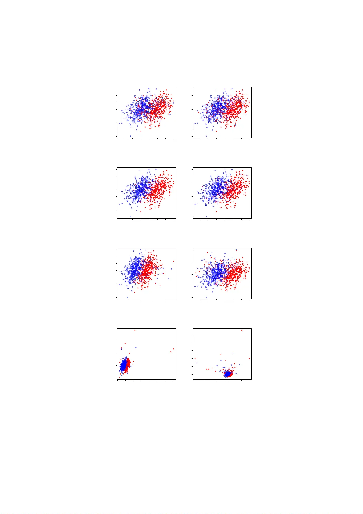
Classi fi cation under Data Con tamination with Application to Remote Sensing Image Mis-registr a tion Donghu i Y an †¶ , P eng Gong §¶ , Aiy ou Chen ‡ , Liheng Zhong §¶ † Departmen t of Statistics § Departmen t of En vironmen tal Science, P olicy and Managemen t ¶ Univ ersit y of California, Berk eley , CA 94720 ‡ Go ogle, Mountain View, CA 94043 ∗ Abstract This work is motiv ated by the p roblem of image mis-registration in remote sensing and w e are interested in determining the resulting loss in the accuracy of pattern classification. A statistical formulation is given where w e prop ose to u se data contamination to mod el the phen omenon of imag e mis-registration. This model is widely applicable to many other types of errors as well, for ex amp le, measurement errors and gross errors etc. The impact of data contamination on classification is studied un der a statistical learning theoretical framework. A closed-form as ymp totic b ound is established for the resulting loss in classification accuracy , whic h is les s than ǫ/ (1 − ǫ ) for data conta mination of an amount of ǫ . Our b ou n d is sharp er than similar b ounds in the domain adapt ation literature and, unlike such b ounds, it applies to classifiers with an infinite VC dimen- sion. Extensive simulatio ns hav e b een conducted on b oth synthetic and real datasets under v arious typ es of data contaminatio ns, including la- b el flipping, feature swa ppin g and the replacement of feature va lues with data generated from a random source such as a Gaussian or Cauch y dis- tribution. Our simulation results show that the b ound we derive is fairly tight. 1 In tro duction A motiv ating example of this w ork is the problem of image mis-reg istration which occurs almost ubiquitously in remote sensing. Image mis-r egistration refers to the pheno meno n w her e the image of int ere s t is ma pp ed or aligned to a wrong p osition. This is usua lly caus ed by error s in the image or data acquisition device or the inaccura cy of the underlying mapping algor ithms whic h try to map data co llected at different scales, at different times, or taken from different ∗ The authors can be co ntact ed at: dh yan@berkeley .edu, penggong@berkeley .edu, Aiy- ouc hen@google.com, lihengzhong@berkeley .edu. This w ork was partiall y done while AC was at Bell Labs, Murr a y H ill, NJ. 1 angles. Figure 1 b elow illustra tes an instance of image mis-r egistration where the imag e is tilted and then shifted by a small a mo un t. Figure 1: The original (left) and the mis-r e gister e d (right) r emote sensing images for a cr opland. Each c olor c orr esp onds to one land class. The pr oblem of ima ge registra tion is of primary imp ortance in remote sens- ing land monitor ing applicatio ns which typically r equire the use of a num b er of images acquired at different times o r time sequence data that can characterize seasona l changes or m ulti-annual similar ities (Defries and T ownshend, 1999 [13]; Liu et al., 2006 [27]). This demands image reg istration and can affect such appli- cations as image classification, change detection, ecolo gical/climato logical/hydrological mo deling (Justice et al., 19 98 [26]; Go ng and Xu, 2 003 [21]) etc. Because ima ge registra tion can never b e p erfectly ma de, a mis-registra tion erro r is inevitable. It has b een sugges ted that mis-reg istration err ors that are less than 0.5 pix e ls are a c c eptable in s ubsequent a nalysis (Gong et al., 1992 [2 0]; T ownshend et al. 1992 [36]; Je nsen, 20 04 [25]). H owev er, this is rarely achiev able and it is thus impo rtant to assess the impact of ima ge mis-re gistration. Of a simila r nature a re er rors due to rounding or the inaccura cy of the mea - suring instruments. Besides , interference fro m electroma gnetic wa ves, clouds o r other unfav orable weather co nditions c an all cause er r ors to the remote sensing images. Additionally , v arious t yp es of h uman error s often factor in where a small amount of arbitrar y erro r maybe thrown in anywhere in the data or any part o f the data can b e missing . Err o rs of this type ar e often called g ross er rors, and are estimated to o ccur in ab out 0 . 1% to 10 % of the data [22]. This estima- tion of the amount of err ors will form the basis for our choice on the amount of data contamination in our sim ulatio n. W e call error s dis cussed ab ove br oadly a s da ta c o nt amina tio n. Data contam- ination can cause a disas trous effect to the data q uality and may fundamentally impact subse quent analys is a nd inference. It is th us of significa nt practical im- po rtance to answer the ques tion: How much do es data c ontamination imp act our analysis (classific ation)? Do curr ent algorithms (classifiers) c ontinue to work or how much do we lose in ac cur acy if a r emote sensing image is mis- r e gister e d or the underlying data ar e c ontaminate d? The goal of the present work aims to shed lights on these questions. T o ga in insights into the na ture of data contamination, in particular the phenomenon of image mis-r egistration, it is highly des ired to appro a ch the pr oblem with a formal mo del and to give some theoretical characterizatio n. This forms the primary motiv ation of the present work. Our fo cus will b e on classifica tion. 2 Assume the data of interest ar e drawn i.i.d. from some pr o bability distr ibu- tion G defined on R p . By treating error s a s contaminations to the pro babilit y distribution G , w e ar rive at the fo llowing sta tistical mo del for data contamina- tion ˜ G = (1 − ǫ ) G + ǫH (1) where ˜ G is the distribution o f the data after contamination and H is a n arbitrary distribution. Mo del (1) is quite genera l, clearly it captures v arious types o f data contaminations we have discussed (not the additive noise though). Note that, in the setting of classification, G is the joint distribution of the attributes and the lab el, thus a co nt aminatio n under mo del (1) can mea n that to the a ttr ibutes, or the lab el, or b oth. The ǫ in (1) ca n b e though t of as the prop o rtion of data (e.g., imag e pixels) that are “ contaminated”, e.g., b eing flipped in lab el or altered with data gener ated under a differen t distribution H . It is known that the effect of imag e mis- r egistratio n is determined by re s - olution, scene structur e and amo un t of r egistration err or (e.g., 0.5 pixe ls or 1 pixel, o r 1 .5 pixels on RMS error ). In mo del (1), we choose to use the pro- po rtion of pixels that are “co nt amina ted” as a measure of the extent of image mis-registr ation. This is to capture the ess ence of ima ge mis- registra tion and to uncover the relationship b etw een the amount o f mis-r e gistration and the re- sulting lo ss in cla ssification accur a cy . This is differe n t from the usual pr actice in the remote sens ing communit y where the image mis-registr a tion is qua n tified in term of a s hift o f a certain num b er of pixels. Since given the same amo un t of shift, the impact on class ification is hig hly sce ne - dependent, e .g., the im- pact would b e dras tically differ e n t for a la rge land consisting mainly of forests and a sma ll land pa rcel formed by co rn fields and rice fields, it would then hardly b e p ossible to establish a ge neric rela tionship b etw een the amount of mis-registr ation and the r esulting loss on the cla ssification accura cy . Our contributions are a s follows. W e pr op ose a statistical mo del for the phenomenon of image mis-r e gistration. This da ta contamination model capture s a wide range of erro rs such as la bel flipping, measurement erro rs, rounding error s and accidental human err ors which o ccur almost ubiquitously in real applications. W e study classificatio n under data contamination in the s tatistical learning framework. A b ound is obtained on the loss of classification accura cy (term this as the data contamination b ound) due to data contamination (to the tra ining da ta) in ter ms of its amo un t. T his b ound a llows o ne to give a conserv ative a ssessment o n if a class o f classifica tio n algorithms, i.e., those which are universally consistent, contin ue to work under data cont aminatio n. The rest of the pap er is orga nized as follows. In Section 2 , we formulate the problem of c lassification under data cont amina tion and obtain a b ound on the loss in classification accura c y in terms o f the amount of data co n tamination. This is follow ed by a discuss ion of rela ted work in statistics, r emote sensing and machine learning in Section 3, and in particular we compare v arious asp ects of our b ound with the finite sample type o f b ounds established in the recently emerging ar ea–domain a daptation. In Sec tio n 4, we conduct extensive sim ula- tions o n the impact of da ta contamination to class ification p erformance of SVM for a n umber of sy nthetic a nd real datase ts under v arious types of data contam- inations. In Section 4.5, we briefly discuss heuristics to estimate the amount of data contamination for the case o f image mis-registra tion. Finally we conc lude in Section 5. In this section, we also co llect r esults fro m the liter ature on the 3 impact of clas sification perfo rmance by AdaBo ost due to lab el flipping; addi- tionally , w e give insight o n us ing da ta contamination as a mo del to under stand co-training , which is pa rticularly useful in situations wher e training data ar e scarce. 2 Classification under data con tamination Classification is an imp ortant problem in pattern recog nition. How ever, a s dis- cussed in Section 1, esp ecially in the context of land-cover, la nd-use mapping, crop yield estimatio n and many other imp or ta n t applications in re mo te sensing, the cla ssification result may b e affected by data contamination. In this section, we will study c la ssification under data contamination with mo de l (1) a nd de- rive a b ound o n the resulting loss in clas sification acc uracy . W e sta rt by an int ro ductio n of the statistical lear ning framework for classification [15]. 2.1 Classification in the statistical learning framework In statistical lear ning, a class ific a tion rule (or classifier ) is defined by a map: X → Y where X is the sample space for observ ations and Y is a finite set of la b els. F or simplicity , we consider throughout a tw o-clas s pr oblem where Y = { 0 , 1 } . Asso ciated with ea c h classifier, there is a perfo rmance measur e ca lle d loss function, denoted b y l ( f , X, Y ). The loss function that is of sp ecial interest is the 0- 1 lo ss, defined as l ( f , X, Y ) =  0 if I { f ( X ) > 0 } = Y 1 otherwise (2) where f is a decision function and I { . } is the indicator function. Her e we call a function f a decision function if a de c ision rule can b e written as I { f > 0 } . Definition. Let P b e the joint probability distribution o f X a nd Y . Then the ris k asso ciated with a decision function f is defined as R P ( f ) = E P l ( f , X, Y ) = P ( Y 6 = I { f ( X ) > 0 } ) . (3) Similarly , the empir ic al risk for a decisio n function f , o n a training sam- ple ( X 1 , Y 1 ) , ..., ( X n , Y n ), can b e obtained by replacing P in the a bove with its empirical distributio n ˆ P n . Fix a pr obability distribution P and a function clas s G , the goa l of classifi- cation is to find a decision rule f ∗ G ∈ G that minimizes R P ( f ), i.e., f ∗ G = arg min f ∈G R P ( f ) . (4) The rule lea rned from the training sample ( X 1 , Y 1 ) , ..., ( X n , Y n ), deno ted by f n , can b e de fined similarly b y subs titution of P with ˆ P n in (4). Definition. Fix a pr obability distribution P . T he function that achiev es the minim um risk, a mo ng all p ossible decision rules, is called the Bay es rule. The co rresp onding risk is called the Bay es risk and is denoted b y R ∗ P . F or the 0-1 loss as defined in (2) and a fixed probability distribution, the Bay es rule is given by β ( x ) = I { η ( x ) > 0 } 4 where η ( x ) = P ( Y = 1 | X = x ) − 0 . 5 is called the Bayes decision function. Definition. A class ific a tion a lgorithm is universally co nsistent if, for all distributions P , R P ( f n ) → a.s. R ∗ P as n → ∞ where a.s. stands for almost surely . Notation. T o simplify notation, we adopt the fo llowing conv ention. Denote R , R G and ˜ R , R ˜ G . Also we use ˜ to indicate a qua n tity a s so ciated with the contaminated distribution ˜ G . In par ticula r, f n and ˜ f n are the class ifiers learned from a training s ample of size n from G a nd ˜ G , resp ectively; and η , ˜ η and η H are the Bay es dec is ion function under G , ˜ G and H , resp ectively . 2.2 A b ound on t he loss of classification accuracy In the standar d setting of statistical lear ning theory , one is int er e s ted in the consistency of a classifier , f n , obtained via empirical risk minimizatio n, that is, R ( f n ) − → R ∗ as n → ∞ . In such a case, the c lassifiers f n are tr a ined and tested with data generated from the sa me probability distributio n G . In the present work, we cons ider a different setting where the pro bability distribution, ˜ G , of the training sample differs from that o f the test sample, G . Of course if G and ˜ G are “ totally” different, then there is no hop e o f le a rning. W e th us make the assumption that G and ˜ G differ by a small amount in the sense of a “small” ǫ under mo del (1). Clearly the rule le a rned from a tra ining sample under ˜ G will b e different from that under G . Since the test s ample is from G , class ifier tr a ined under ˜ G would t ypica lly have a larg er class ification error . One imp ortant question is, how m uch a dditional classificatio n erro r will be intro duced if the c la ssifier is trained on a sample from ˜ G (instea d of G ) when testing o n a sample generated fro m G . Really we wish to know how muc h R ( ˜ f n ) is different fr om R ( f n ) as n → ∞ for ǫ small. As we do not hav e access to data from G , a natura l proxy for R ( f n ) is R ∗ since R ( f n ) → R ∗ as n → ∞ for consistent classifier s f n . W e s ta rt b y the following r isk decomp osition R ( ˜ f n ) − R ∗ = R ( ˜ f n ) − R ( ˜ η ) + R ( ˜ η ) − R ∗ . (5) The R ( ˜ η ) − R ∗ term in (5) can b e b ounded b y a term that dep ends only on the amount of contamination, ǫ , under some w eak assumptions . This is stated as Theorem 1 . The term R ( ˜ f n ) − R ( ˜ η ) can b e shown to v anish as the training sample size increases if the underlying cla ssifier is universally consistent. This is s tated as Theorem 2. Note that here the co n vergence rate may b e different for different types of classifiers . Theorem 1. If g ( x ) , the pr ob ability density function of G , exists, then for data c ontamination with any distribution H , R ( ˜ η ) − R ∗ ≤ ǫ 1 − ǫ , wher e the e quality holds if and only if the fol lowings ar e true 5 a) ǫ = 0 . 5 − R ∗ 1 − R ∗ , h ( x ) = | η ( x ) | g ( x ) 1 − 2 R ∗ , and b) P H ( Y = 1 | X = x ) = 1 when η ( x ) < 0 , and 0 otherwise. Remark. 1. The b ound as s tated in Theorem 1 is sha rp as it is achiev able under a sp ecial case as noted in the statement of the theorem. 2. A r elated data con taminatio n mo del is as follows. d ˜ G ( x ) = [1 − ǫ ( x )] dG ( x ) + ǫ ( x ) dH ( x ) (6) such that 0 ≤ ǫ ( x ) ≤ ǫ < 1 for some p ositive constant ǫ where G, H , ˜ G are probability distribution functions. Mo del (6) allows the amo unt of data contamination to b e da ta dep endent a s lo ng a s the amount is unifor mly smaller than a constant. Similar r esult a s Theorem 1 can b e obtained. T o prepare for the pro of of Theorem 1, w e have the following lemma. Lemma 1. L et f b e a de cision function. F urther assu me P ( f ( X ) = 0 ) = 0 . Then R ( f ) = 0 . 5 − E [ η ( X ) . sign ( f ( X ))] wher e sig n ( x ) = 1 if x > 0 and − 1 otherwise. Pr o of. Note that we c an write R ( f ) = E G   Y − I { f ( X ) > 0 }   . Thu s R ( f ) = E  Y .I { f ( X ) < 0 }  + E  (1 − Y ) .I { f ( X ) > 0 }  = 0 . 5 + E  ( Y − 0 . 5) .I { f ( X ) < 0 }  + E  (0 . 5 − Y ) .I { f ( X ) > 0 }  = 0 . 5 − E [ η ( X ) . sign ( f ( X ))] . The p osterio r pro bability ˜ η ( x ) + 0 . 5 under the contaminated distribution ˜ G can be written as ˜ η ( x ) + 0 . 5 = [1 − α ǫ ( x )]( η ( x ) + 0 . 5) + α ǫ ( x )( η H ( x ) + 0 . 5 ) where α ǫ ( x ) = ǫh ( x )[(1 − ǫ ) g ( x ) + ǫh ( x )] − 1 . Here g a nd h ar e the contin uous density o r discr ete proba bilit y functions co rre- sp onding to G and H , re spe c tively . Then ˜ η = (1 − α ǫ ) η + α ǫ η H . 6 Pr o of of The or em 1. By Le mma 1, w e have R ( ˜ η ) − R ∗ = E [ η ( sig n ( η ) − sig n ( ˜ η ))] = 2 E  | η | .I { η ˜ η < 0 }  . Next notice that, if η ˜ η = α ǫ η 2  (1 − α ǫ ) α ǫ + 2 η H 2 η  < 0 , then this implies 2 | η | ≤ α ǫ (1 − α ǫ ) = ǫ 1 − ǫ h ( x ) g ( x ) . Hence, R ( ˜ η ) − R ∗ ≤ 2 E  | η | .I { 2 | η | ≤ ǫ 1 − ǫ h ( X ) g ( X ) }  (7) ≤ ǫ 1 − ǫ E h ( X ) g ( X ) (8) = ǫ 1 − ǫ . The e quality in (7) holds if and only if η H = − 1 2 , or, P H ( Y = 1 | X = x ) = 1 when η ( x ) < 0, a nd 0 otherwise, i. e. fo r the same obse r v ation X = x , the worst rule under H a ssigns a completely o ppo sitive clas s mem b ership w.r.t. that under G . F urther, the eq uality in (8) holds if and only if 2 | η ( x ) | = ǫ 1 − ǫ h ( x ) g ( x ) , which implies 2 E | η | = ǫ 1 − ǫ since R h ( x ) dx = 1. Thus, ǫ = 2 E | η | 1 + 2 E | η | = 0 . 5 − R ∗ 1 − R ∗ by Lemma 1. This co ncludes the pr o of. Theorem 2. S upp ose a classific ation algorithm is universal ly c onsistent . Then, under data c ontamination mo del (1) , we have R ( ˜ f n ) → R ( ˜ η ) as n → ∞ . The pro of o f Theore m 2 relies o n the following lemma. Lemma 2 . Assum e P ( η ( X ) = 0) = 0 . If R ( f n ) → R ∗ , then the de cision induc e d by f n c onver ges to t he Bayes rule in pr ob ability as n → ∞ . 7 Remark. Theorem 2 of Bartlett a nd T ewari [3] implies that the decision rule g iven by SVM conv erges to the Bayes rule. Lemma 2 is mor e genera l in that it applies to all consistent rules. Pr o of. Without loss of generality , ass ume the decision function f n is a lready centered, i.e., the corres po nding decision rule can b e written as I { f n > 0 } . F ro m Lemma 1, we hav e R ( f n ) = 0 . 5 − E ( η ( X ) ∗ sign( f n ( X ))) . Let ξ n ( x ) = | sign( η ( x )) − sign( f n ( x )) | , then ξ n ( x ) takes t wo v alues { 0 , 2 } . W e hav e R ( f n ) − R ∗ = E ( η ( X )) [sign( η ( x )) − sign( f n ( x ))] = E | η m ( X ) | .ξ n ( X ) . Thu s, P ( ξ n ( X ) = 2) → 0 by assumption R ( f n ) → R ∗ as n → ∞ . That is, I { f n ( X ) > 0 } conv erges to I { η ( X ) > 0 } in pro bability as n → ∞ . Pr o of of The or em 2. By universal consistency and Lemma 2, we have Z I { sign ( ˜ f n ( X )) 6 = sign ( ˜ η ( X ) ) } d ˜ G ( x ) → 0 . Thu s Z I { sign ( ˜ f n ) 6 = sign ( ˜ η ) } dG → 0 , implying that, as n → ∞ , R ( ˜ f n ) → R ( ˜ η ) . By risk decomp osition (5) as well as Theo rem 1 and Theo rem 2, we arrive at a sharp asymptotic da ta co ntamination b o und as ǫ 1 − ǫ + O ( c ( n )) . (9) where c ( n ) = R ( ˜ f n ) − R ( ˜ η ) indicates the rate of conv ergence with c ( n ) → 0 as n → ∞ . Bound (9) implies that, when the amount of data contamination is “small” , i.e., ǫ → 0 , we ca n make | R ( ˜ f n ) − R ∗ | → 0 . That is, as long as a cla s sifier is co nsistent in the standard s etting and the amount of contamination is small in the sense of a small ǫ , this classifier suffers very little from data contamination. This explains why , empirica lly , classifier s such as SVM or others work w ell even when a sma ll fraction of lab els are ran- domly flipp ed. Theorem 2 r elies on the universal consistency of a classifier. F or tuna tely , several of the currently most p opular classifiers ar e universally consistent, for example, SVM [33] and Adabo o st with ea rly stopping [4]. 8 3 Related w ork The study of data ana lysis and statistical inference under data contamination has b een a long-s tanding resear ch topic in statistics and machine lea rning. The earliest work can b e tr a ced back to at least a half century ago, see, fo r example, T ukey [37] for a survey o n sa mpling from contaminated distribution. Extensive studies hav e b een carried out since under the name of ro bust estimatio n ([24, 22]), meas ur ement error mo del ([18, 9, 14]) etc. How ever, work alo ng this line concerns primar ily problems on regres sion or estimation. Relev ant literature in remo te sensing , how ever, has b e e n sparse. Swain el al [35] inv estiga ted the impact o f image mis- r egistratio n to class ification. How- ever, this work is purely empirical and their r e s ults dep end highly on the un- derlying scenes in the imag e ; for example, even under the same amount of mis-registr ation, the impact would b e considerably different on imag e s formed primarily by la r ge forest lands and those for med by many small pa tch es of dif- ferent la nd types such a s corns and plants. Additionally , T ownshend el a l [36] considered the impact of image mis- registra tion to change detection. Xu et al [39] study parameter estima tio n for a simple linear mo del under measurement error s due to a mismatc h o f lo cations and scales. Related machine learning literature is muc h richer. Such work can be br oadly divided into tw o stag e s . The first s tage, roughly b efore year 20 05, mo stly deals with data co n taminatio n in the form of la be l flipping and e mpir ical study o f its impact on the p erfor mance of v ario us classifiers. This includes Dietterich [16] and Breiman [8] which ev alua te the r obustness of learning algorithms such as bagging , AdaBo ost and Ra ndom F o r ests against lab el flipping . Other work includes ([30, 32, 41]) and r eferences therein. The second or the cur rent stage, which is clos ely rela ted to the present work, dea ls with domain ada ptation. Do- main adaptatio n is a broa der c o ncept than data co n taminatio n in that it do es not spe c ify explicitly the nature of the difference b etw een the source (or train- ing) distribution and the tar get (or test) distribution a s long as their difference is small wher eas data co n taminatio n a lmost exc lusively refer s to mo del (1). There hav e b een numerous pap ers published on do main adaptation, including appli- cations, theory and metho ds, and it is beyond the s c o pe of the pre s ent pap er to g ive a detaile d account her e. W ork that is closest to ours include ([5, 28]) (see also r eferences there in). In particular, Ben-David et al [5] established the following b ound. Theorem 3 ([5 ]) . L et H b e a hyp othesis sp ac e of VC dimension d . If U S , U T ar e unlab ele d samples of size m ′ e ach, dr awn fr om the s our c e distribution D S and the tar get distribution D T r esp e ctively, then for any δ ∈ (0 , 1) , with pr ob ability at le ast 1 − δ (over the choic e of the samples), for every h ∈ H , the differ enc e b etwe en the err or r ates ǫ S and ǫ T satisfies ǫ T ( h ) − ǫ S ( h ) ≤ 1 2 ˆ d H ∆ H ( U S , U T ) + 4 r 2 d log(2 m ′ ) + log (2 /δ ) m ′ + λ wher e λ is define d by λ = arg min h ∈H [ ǫ S ( h ) + ǫ T ( h )] with t he subscripts S, T indic ating quantities r elate d to t he sour c e and tar get, r esp e ctively. 9 The b ound established in [28] is similar in nature which replaces the VC dimension in [5] with the Rademacher complexity [2]. How ever, there are im- po rtant differences b etw een the bound in Theorem 3 or that in [28] a nd our s (i.e., Theor em 1). (1) The nature of bo unds is differ en t. The b ounds in ([5, 2 8]) ar e finite s a mple learning g eneralizatio n t yp e of b ounds while our b ound is a large s ample bo und (i.e., asymptotic b ound). (2) The quality of the b ounds is different. The b ounds in [5] ar e union b ounds that r e ly on the V apnik-Chervonekis (VC) dimension [38], and are often quite lo ose ([28] uses the Ra demacher complexity [2] but s till quite lo ose). In con tra st, our b ound is a shar p b ound asymptotically . Assume the underlying function class has a finite V C dimension and let m ′ → ∞ , then the b ound in Theore m 3 be c omes ǫ + λ , which is lo o s er than our bo und ǫ/ (1 − ǫ ) ≈ ǫ for small ǫ . Since the λ term dep ends on the difficult y of the underlying problem a nd generally do es not v anis h, in no w ay would the bo unds in [5 ] imply o urs. T o b etter appr e c iate the differenc e in the quality o f the b ounds when the sample size inc r eases, we will show a n exa mple where the data is generated by a tw o-co mpo nent Gaussian mixture and co n taminated by Cauch y data (See Section 4 for details on the Gaussian mixture and the Cauch y). Since it is no t eas y to directly compute λ , we replace it with its low er bo und arg min h ∈H ǫ S ( h ) + arg min h ∈H ǫ T ( h ), which are estimated as the erro r r ates of SVM o n the da ta when the training sample siz e is la rge. Figure 2 shows the asymptotic da ta co nt aminatio n b ounds o f our s and that established in [5] for the amount of data co n taminatio n v arying from { 0 . 01 , 0 . 02 , 0 . 0 3 , 0 . 04 , 0 . 05 , 0 . 10 } . One ca n see that her e the Ben- David et al bo und [5] is muc h lo oser than ours , and for this particular Gaussian mixture data, the Ben-David et a l b ound is not very informative as it quickly a pproaches 0 . 5. 0 0.01 0.02 0.03 0.04 0.05 0.06 0.07 0.08 0.09 0.1 0 0.1 0.2 0.3 0.4 0.5 0.6 0.7 Amount of data contamination (Gaussian Mixture) Data contamination bounds Our bound Bound of Ben−David et al Figure 2: Comp arison of data c ontamination b oun d for Gaussian mix t ur e data with ǫ ∈ { 0 . 01 , 0 . 02 , 0 . 03 , 0 . 04 , 0 . 05 , 0 . 10 } . 10 (3) Whereas our bound a pplies only to univ ers ally consistent clas sifiers, the bo und in [5] a pplies only to classifier s from a function class with a finite V C dimension. This is a limitation that cannot be ov erlo oked. F o r exa m- ple, the function class co rresp onding to the Gaus s ian kernel (see discussio n after example 1.9 in [3 4] a nd the fact that the Gauss ian kernel is a uni- versal kernel), or the p olynomial kernel (if no upper bo und is impo sed on the degr ee o f p olynomia ls), or the one neares t neighbo r class ifie r , o r the tree-based classifier (without r e gularizatio n) all hav e an infinite VC dimen- sion. Consequently , the b ound in ([5]) excludes some of the b est classifiers av a ilable to day , including SVM with the Gaussian kernel, Bo o sting (or Bagging [7]) o n tree-bas ed classifie r s etc while o ur bo und clea rly do es not hav e such a r estriction. 4 Exp erimen ts Empirical studies a re p erfor med on three different types of datasets, 3 synthetic datasets, 10 UC Ir vine data sets [1] and a simulated re mo te sensing image. F or each datas e t, four different type s of da ta contaminations are applied to the training set and clas s ification a ccuracy e v aluated on the uncont aminated test set. SVM is used as the underlying class ifie r due to its universal consis tency [33] and the av ailability of a wide ly used s oft ware implementation (libsvm [10]). The five differe nt types of data co nt amina tio ns are as follows. C 0 . Randomly flip the lab els o f a rando mly sele c ted subset o f observ ations from a fixe d class . C 1 . Randomly flip the lab els o f a rando mly sele c ted subset o f observ ations from all cla sses. C 2 . Randomly selec t a subs et of observ ations and r eplace the feature v alues of ea ch with tha t o f a randomly chosen observ ation (the lab els a re kept). Call this feature swapping. C c . Replace a ra ndomly selected subset of observ ations with Cauchy data with the lab els k ept. C g . Replace a r andomly selected subset of observ ations with Gaussia n data with the labe ls kept. C 0 , C 1 , ..., C g are used to simulate data contamination of different natures . • C 1 and C 2 are expressly designed to simulate image mis-regis tration, whic h we b elieve capture imp ortant asp ects o f image mis-r egistratio n. • C c and C g are used to sim ulate gr o ss error s. C g is for erro rs with a Gaussian nature while C c is for error s with a heavy tail, tha t is, the err or could b e very large a nd this is to simulate acc iden tal human erro r, for example, a shift in decima l place of a num b er. • Additionally , we als o attempt to simulate extr emely la rge e rrors by s caling the cen ters of the Gaus s ian and Cauch y by a factor of 100, that is, the centers ar e multiplied by 100 co or dinate-wisely . The s e are denoted by C g 100 and C c 100 , re s pec tively . 11 −3 −2 −1 0 1 2 3 −4 −3 −2 −1 0 1 2 3 Figure 3: Sc atter plo t of 1000 observations gener ate d i.i.d. fr om Gaussian N ( µ, Σ) with µ = (1 , 0) and Σ = A t A with entries of A gener ate d i.i.d. fr om U [0 , 1] . Data fr om the two classes ar e re pr esente d as diamonds and solid cir cles, r esp e ctively. • C 0 is used to simulate a class of unfav ora ble situations where data con- tamination occur s in par t of the data space. Such cases t ypically make classification more challenging. In contrast, o ther simulations ar e more or less av erag e cases as the data co ntamination o ccurs uniformly acr oss the whole data space. F or C g , the r eplacement Gauss ian data is generated i.i.d. fr om N ( µ, Σ) with µ and Σ calculated empirically on the non-contaminated training set. F or C c , the Cauch y data is generated i.i.d. according to Z/W, for Z ∼ N ( µ, Σ) , W ∼ [Γ(0 . 5 , 2)] 1 / 2 with Z a nd W independent wher e Γ(0 . 5 , 2) is a random v ar ia ble generated from a Gamma distribution with parameters 0 . 5 and 2. F or ea ch r un, µ is g e nerated uniformly from the interv al [min ( X ) , max( X )] and Σ estimated e mpirically from the tra ining set. F or a n illustration of the effect of these different types of data contamination, see Figur e 3 for the o riginal data and Figur e 4 for the da ta after contamination of different t yp es. 4.1 Syn thetic data The three synthetic da tasets used in our exp eriment a re the Ga us sian mixtur e data, the four -class and the nested-squar e data. The Gaussian mixture data ar e used to simulate cases with a linear dec is ion bo undary while the four-clas s a nd the nested-squar e datasets are for ca ses where the decision b oundary is hig hly nonlinear and non-convex. F or each of the 3 datas ets, we take 80% for training and the rest for test. Then 100 instances of data contamination are a pplied and loss in c lassification accuracy are averaged. This is rep eated and res ults 12 −3 −2 −1 0 1 2 3 −4 −3 −2 −1 0 1 2 3 C1 (5%) −3 −2 −1 0 1 2 3 −4 −3 −2 −1 0 1 2 3 C1 (10%) −3 −2 −1 0 1 2 3 −4 −3 −2 −1 0 1 2 3 C2 (5%) −3 −2 −1 0 1 2 3 −4 −3 −2 −1 0 1 2 3 C2 (10%) −2 0 2 4 −4 −3 −2 −1 0 1 2 3 Cg (5%) −3 −2 −1 0 1 2 3 −4 −2 0 2 4 Cg (10%) −5 0 5 10 15 20 25 30 −5 0 5 10 Cc (5%) −20 −10 0 10 0 10 20 30 40 50 Cc (10%) Figure 4: Il lustra tion of the effe ct of differ ent typ es of data c ontamination. The original Gaussian data ar e displaye d in Figur e 3. The 4 r ows of plots c orr esp ond to C 1 , C 2 , C g , C c , r esp e ctively and figur es in the left and right c olumns ar e for data c ontamination at 5% and 10% , r esp e ct ively. Data fr om the two classes ar e r epr esente d as diamonds and solid cir cles, r esp e ctively. 13 are averaged. The Gauss ian kernel is used with SVM for all three synthetic datasets. The Gaussian mixture data are generated according to the following ∆ N ( µ, Σ 10 × 10 ) + (1 − ∆) N ( − µ, Σ 10 × 10 ) with P (∆ = 1) = P (∆ = 0) = 1 2 and Σ 10 × 10 = A T A for en tries o f A genera ted i.i.d. uniform from [0 , 1], with µ = (0 . 5 , ..., 0 . 5) T . Data p oints with ∆ = 1 are assigned lab el 1 and those with ∆ = 0 are assigned lab el 2. The sample size for the training set and test set are 1000 and 2000, resp ectively . Loss in classifica tio n accuracy under data contamination of different types and at different a mounts are shown in Fig ur e 5. Note that here we are using only the fir st term in (9) as an estimate of the ov erall loss in c lassification accura c y while ig noring the s e c ond term, thus when the training sample s iz e is not la rge enough, some a djustmen t (in the order of O ( c ( n ))) might b e required. 0.01 0.02 0.03 0.04 0.05 0.06 0.07 0.08 0.09 0.1 0 0.02 0.04 0.06 0.08 0.1 0.12 0.14 0.16 0.18 0.2 Amount of data contamination (Gaussian Mixture) Loss in accuracy Theoretical bound C0 C1 C2 Cg100 Cg Cc100 Cc Figure 5 : Empiric al and the or et ic al data c ontamination b oun d for data gener ate d fr om a Gauss ian mixtu re with ǫ ∈ { 0 . 0 1 , 0 . 02 , 0 . 03 , 0 . 04 , 0 . 05 , 0 . 10 } . 0 20 40 60 80 100 120 140 160 180 200 0 20 40 60 80 100 120 140 160 180 200 50 60 70 80 90 100 110 120 130 140 150 50 60 70 80 90 100 110 120 130 140 150 Figure 6: The four-class and n este d-squ ar e data. Differ ent c olors c orr esp ond to p oints fr om differ ent classes. The four -class a nd nested- s quare da tasets were o r iginally used to demon- strate the sup erior p erforma nce of a class of pro jectable classifier s for data with a highly complex decisio n bo undary [23]. Figur e 6 is a plot of these t wo da ta sets 14 and the data contamination bounds are shown in Figure 7. Note tha t the b ound as established in (9) is for 2-class classificatio n. When ther e are multiple cla sses, we can g et a b ound by rep eatedly apply the the 2-cla ss b ound. Let the class distribution b e denoted by { w 1 , ..., w J } such that w 1 ≥ ... ≥ w J . Then w e g et the following multi-class b ound ǫ 1 − ǫ  1 + ( w 2 + ... + w J ) α + ... + ( w { J − 1 } + w J ) α J − 2  where α = 1 − ǫ 1 − ǫ and ǫ is the mount o f contamination. This is used as the theoretical b ound in our s im ulations when there are more than t wo classes . 0.01 0.02 0.03 0.04 0.05 0.06 0.07 0.08 0.09 0.1 0 0.02 0.04 0.06 0.08 0.1 0.12 0.14 0.16 0.18 0.2 Amount of data contamination (4−class) Loss in accuracy Theoretical bound C0 C1 C2 Cg100 Cg Cc100 Cc 0.01 0.02 0.03 0.04 0.05 0.06 0.07 0.08 0.09 0.1 0 0.05 0.1 0.15 0.2 0.25 0.3 0.35 0.4 Amount of data contamination (Nested Square) Loss in accuracy Theoretical bound C0 C1 C2 Cg100 Cg Cc100 Cc Figure 7: Empiric al and the or etic al data c ontamination b ound for the 4-class and the neste d-squar e datasets with ǫ ∈ { 0 . 0 1 , 0 . 02 , 0 . 03 , 0 . 04 , 0 . 05 , 0 . 10 } . 4.2 UC Ir vine datasets A total of 10 datasets ar e taken fro m the UC Irvine Machine Lear ning Rep osi- tory [1] in our exp eriment. A summar y o f these datasets is provided in T able 1 and more details can be found fro m [1]. T able 1: Summary of the UC Irvine datasets use d in our exp eriment. T ra ining T esting F eatures Classes imag e S eg 210 2100 19 7 V owel 528 462 10 11 S atell ite imag es 4435 2000 36 6 Gla ss 214 – 10 6 V ehicl e 946 – 18 4 German cr edit 1000 – 24 2 Y east 1484 – 8 10 W ine q u al ity 1599 – 11 6 M usk 6 598 – 1 68 2 M ag i c g amma 19020 – 10 2 Some data sets come with predeter mined training and test sets, which in- cludes the image segmentation, vo wel a nd satellite image datasets. Otherwis e 15 we split the data into a training and test set. F o r small to medium sized datasets, i.e., Glass, V ehicle, German C r edit, Y east and Wine Qua lit y (r e d wine), we take 80% of the data for tra ining and the r est for test. F or larg e datasets, i.e., the Musk and Magic Gamma T elescop e, 20% and 10 %, res p ectively , of the data are set aside for training and the re s t for test. F or ea ch dataset, 100 instances of data contamination ar e applied to the tra ining s et and the res ulting data contamination bo unds are averaged. This is r epe a ted and results av era ged. The Ga us sian kernel is used for all except the ima ge segmentation dataset where a p olyno mia l kernel with degree 3 is used. T uning pa rameters for SVM are chosen so that the cla ssification p erformanc e ma tches that rep orted in the literature (se e , for example, refer ences cited in the description of ea ch data set in [1 ]). Some da tasets a r e linearly scaled to [0 , 1] so as to s pee d up the painfully slow o ptimization of the SVM pack a ge; this includes the Musk , Ma g ic Gamma, Satellite image, V ehic le , and the Wine qua lit y dataset. The da ta contamination bo unds by SVM on the UC Ir vine datasets are plotted in Figure 8. 0.01 0.02 0.03 0.04 0.05 0.06 0.07 0.08 0.09 0.1 0 0.02 0.04 0.06 0.08 0.1 0.12 0.14 0.16 0.18 0.2 Amount of data contamination (Musk) Loss in accuracy Theoretical bound C0 C1 C2 Cg100 Cg Cc100 Cc 0.01 0.02 0.03 0.04 0.05 0.06 0.07 0.08 0.09 0.1 0 0.05 0.1 0.15 0.2 0.25 Amount of data contamination (Glass) Loss in accuracy Theoretical bound C0 C1 C2 Cg100 Cg Cc100 Cc 0.01 0.02 0.03 0.04 0.05 0.06 0.07 0.08 0.09 0.1 0 0.05 0.1 0.15 0.2 0.25 Amount of data contamination (Vehicle) Loss in accuracy Theoretical bound C0 C1 C2 Cg100 Cg Cc100 Cc 0.01 0.02 0.03 0.04 0.05 0.06 0.07 0.08 0.09 0.1 0 0.02 0.04 0.06 0.08 0.1 0.12 0.14 0.16 0.18 0.2 Amount of data contamination (German Credit) Loss in accuracy Theoretical bound C0 C1 C2 Cg100 Cg Cc100 Cc 0.01 0.02 0.03 0.04 0.05 0.06 0.07 0.08 0.09 0.1 0 0.05 0.1 0.15 0.2 0.25 0.3 0.35 0.4 Amount of data contamination (Wine Quality) Loss in accuracy Theoretical bound C0 C1 C2 Cg100 Cg Cc100 Cc 0.01 0.02 0.03 0.04 0.05 0.06 0.07 0.08 0.09 0.1 0 0.05 0.1 0.15 0.2 0.25 0.3 0.35 0.4 Amount of data contamination (Image Segmentation) Loss in accuracy Theoretical bound C0 C1 C2 Cg100 Cg Cc100 Cc Figure 8: Empiric al and the or etic al data c ontamination b ound for UC Irvine datasets (only 6 of them ar e shown her e so that they c an b e plac e d in the same p age, t he r est ar e similar) with ǫ ∈ { 0 . 0 1 , 0 . 02 , 0 . 03 , 0 . 04 , 0 . 05 , 0 . 10 } . 16 4.3 Remote sensing image The re mo te sensing imag e used in the ex per iment is a bo ut a cr opland with 5 different land-use classes. The image size is 596 pixel by 529 pixel. The features of int ere st a re taken from the annual vegetation index time series (see Figur e 9) at an interv al o f 30 days a mong which 1 0 a re used with each cor resp onding to one scene of image at a differe n t time of the y ear . The v egeta tion index is an optical measure of vegetation canopy gree nness and is closely rela ted to the photosynthetic p otential of pla n ts. F or each pixel, rando m noises, genera ted from Gaussia n N (0 , 0 . 1 2 ), ar e applied. Figure 9: The annual ve getation index. T he x-axis is the day of a ye ar and differ ent c olors indic ate differ ent land classes. T o simulate the acquisition of remo te sensing images, the following pro c edure is p erformed on each of the 1 0 scenes of image. 1. Rotate a ll images c lo ckwisely by 1 0 degre e s. 2. Re-sample each scene o f image using a randomly gener ated offset fro m N (0 , 0 . 1 2 ). 3. Remov e the blank edges in all imag es that are caused by r otation and re-sampling. In Step 2 of the ab ov e, o ffsets are gener ated from the standar d Ga ussian and a bilinear interpolatio n [19] is applied during re-sa mpling. As a result, 24 7 pixel by 2 33 pixel multi-tempor a l vegetation index images for the c r opland of int ere st are g e ne r ated. T o assess the impact of image mis-regis tration to the tas k of classificatio n, t wo mis-regis tered images (corresp onding to Case I a nd I I in T able 2 , res pec - tively) ar e generated under differ en t levels o f mis-regis tr ation (r oughly corr e- sp onding to 3% and 4% data co n taminatio n, resp ectively). The SVM cla ssifier is trained on a sa mple fro m the origina l image and the mis-re gistered image, resp ectively , and then test on a sample taken from the orig inal imag e. W e use the da ta in a simila r fashion a s the 5-fold cross- v alidation, i.e., select 4 folds for training and rest for testing. T able 2 rep or ts the cla ssification accuracy . W e 17 T able 2: A c cu r acy of SVM for the cr opland r emote sensing image un der differ ent amount of image mis-r e gistr ation. Each of t he first 5 c olumns c orr esp onds to one of the 5 folds. F old 1 2 3 4 5 Average Or ig inal 98.13 9 8.14 97 .90 97.9 4 9 7.98 98.02 Case I 98.08 98.1 1 97.9 2 97.94 97 .98 9 8.01 Case I I 98.0 9 9 8.10 97 .92 97 .92 97.96 97.99 can see that, in bo th cas e s, the loss in class ification a ccuracy is small and can be well b ounded by our theore tical predication. It is known that, fo r e x ample b y b o otstr ap, the effect of mis-reg istration on image classifica tion v arie s with the rela tive size of the ground ar ea corresp onding to a n imag e pixel (call this the pixel size) and the actua l homo g eneity (lar ger nu mbers corresp ond to mo re homogeneity) o f an ar e a . If the ratio of these tw o nu mbers is small, then the damag e of mis-registr ation is small, otherwis e it is large. Since we are using a cr op field here a nd the c o rresp onding pixel size is m uch smaller than that for the crop field, the effect o f data contamination is small. If the pixel size is close to the actual o b ject size, then mis- registra tion of half a pixel may ca use more damages. 4.4 Some empirical results on Adab o ost So far SVM has b een used as the under lying class ifier in our exp er iment, other universally consistent classifier s such as Adab o ost ar e applicable as well. In- stead of rep eating the ex per iment for AdaBo ost, we collect results found in the literature [17, 16, 8] and summar ize in T able 3. Note here we simply adopt the existing res ults and this corr esp onds to taking ǫ = 0 . 0 5 only . T able 3: Err or r ates of A dab o ost on some UC Irvine datasets wher e 90% of the data ar e use d as the tr aining set . R esults ar e shown for the origina l data and when 5% of the class lab els in the tra ining set ar e r andomly flipp e d (un iformly into an alternate class). Re sult s ar e adopte d fr om [8 , 17, 16] and t hen c onverte d. Original data 5% la bels flipped Difference Gla ss 22.00% 22.35% 0.35% B r east cancer 3.20% 4.58% 1.38% D iabetes 26.60% 28.41% 1.81% S onar 15.60% 17.96% 2.36% I onspher e 6.40% 8.17% 1.77% S oyb e an 7.57% 9.61% 2.04% E coli 14.80% 15.91% 1.11% V otes 4.80% 7.14% 2.34% Liv er 30 .70% 33.86% 3.16% 18 4.5 Estimating the amoun t of data contami nation Using data contamination bo und (9), we can estimate the loss in accur a cy for classifiers tra ined with contaminated data. The r e maining question is to give a (rough) estimate of the amount of data co n taminatio n. This is a question we would like to leave to future work. In the specia l ca se of image mis-registration, we pr op ose t wo simple heuris tics for estimating the amo un t of data contamination. Both are ba s ed on the heur is - tic that the ima ge pixels a ffected by mis-reg istration are ro ughly those nea r the bo undary b etw een different land classes. Thus the prop or tion of bounda ry pix- els s e rves as a go o d indication on the amount of data cont aminatio n. Here the underlying a ssumption is that the pro po rtion of bo undary pixels a re ro ug hly the same in the true and the mis-reg is tered images. One approach is based on sampling. A num b er , say 1 00 to 2 00, o f pixels are rando mly sa mpled from the image, we then count the prop ortion of pixels that fall on the b ounda ry by vis ual insp ection. Another estimate is based on the classificatio n results by a cla s sifier tra ined on the contaminated data. F o r each pixel, we deter mine if it is on the b oundary by the following heuris tic. F or each pixel in the image , take a 3 × 3 patch centering on it. If ther e are a t least t wo pixels within the patch having a differe nt class lab els from the rest, then declare the pixel at the center of the patc h to b e on the b oundary . 5 Conclusion and discussion W e formulate the pr oblem of image mis- registra tion as data co nt amina tio n and equip it with a statistical model. This mo del captures a v ery ge neral class of error s, for insta nce, meas urement er rors and gro ss error s that ca n b e formu- lated as label- flipping, feature-swapping, or feature replacement by any prop er distributions. Under a statistical lea rning theor etical framework, w e derive an asymptotic b ound for the lo ss in classification a ccuracy due to da ta contamina- tion. One nice featur e ab out this b ound is that, it is ess ent ially distribution-free th us it applies to all different types of da ta. Extensive s im ulations on b oth sy n- thetic and rea l data sets under v a rious t yp es of da ta co nt amina tio ns show that the data contamination b ound we derive is fair ly tight. Compared to simila r bo unds in the domain adaptatio n literature, o ur bo und is sharp er and, unlike such b ounds, our b ound applies to classifiers with an infinite VC dimension. As w e hav e alrea dy discus sed, o ur data contamination mo del ca n capture v ario us types o f er rors such as imag e mis-registra tion, lab el noise and acciden- tal human er rors. Beyond that, we can also use data contamination as a us eful device. W e g ive her e an exa mple in the se tting of c o -training ([40, 6, 11]). Empirically , it has been shown that co -training ca n significantly b o ost the clas- sification ac c ur acy when the training sample s ize is extremely small, e.g., 12 in [6] for web page classifica tion and 6 in [29] for newsgr oup cla ssification. Theo- retical work hav e b een ca rried o ut to understand the success of co-training (see, for instance, [6, 12]). W e pr ovide here a different per sp ective. In co - training, starting from a small amount of la bele d examples, the al- gorithm pr o gressively enlarg es the lab eled s e t by transferring those examples which are or iginally unlab eled but are cla ssified with high confidence by the classifier built fro m the la b eled data av a ilable so far . This amounts to enlar g - 19 Figure 10 : The b enefit of c o-t r aining. E rr ∗ denotes the Bayes err or r ate. ing the la be le d set with a small amount o f la be l noise; the lab el no ise here is small b ecause those examples which are b eing trans fer red ar e classified with high confidence. Assume at certa in p oint we have n ex amples in the lab eled se t and assume n is larg e, then, by our analysis (c.f. (9) ), the additional classifica- tion erro r w.r.t. that resulting from a clea n lab eled set (of siz e n ) is no more than ǫ/ (1 − ǫ ) + O ( c ( n )) for c ( n ) → 0 as n grows. Thus, E rr (Bayes clas sifier on G ) ≤ E rr (Class ifier lea rned on n observ a tions from ˜ G ) ≤ E rr (Bayes clas sifier on G ) + ǫ 1 − ǫ + O ( c ( n )) where E r r deno tes the err or rate. Here, we use G and ˜ G to denote the data with clean lab el and that c o nt aining lab els ass igned by the co-training a lgorithm, resp ectively . It is clear that the erro r rate achieved b y co-tr aining equa ls tha t by a classifier lea rned on n obser v ations fro m ˜ G . How ever, it is often the case that the er r or rate by a classifier learned on l la bele d exa mples from G is typically m uch larger, i.e., E rr (Class ifier lea rned on l examples fro m G ) ≫ E r r (Bay es classifier on G ) + ǫ 1 − ǫ + O ( c ( n )) (10) if l is small, ǫ is s mall a nd n is la r ge. The gap b e t ween the tw o E rr terms in (10) is the p otential “b enefit” of c o -training a s illustrated in Figur e 10. This explains why co -training may b e feasible w ith a small amo unt of initial lab eled examples. Since the ga p in (10) s hr inks a s l incr eases, this, on the other hand, explains why co- tr aining may no t help m uch when the initial lab eled se t is large. A limitation of our data co n taminatio n mo del (1) is that, in mo deling the phenomenon of ima ge mis-regis tr ation with a da ta contamination model, i.i.d. contaminations a re assumed. Howev er, in pra ctice the mis-r egistered image pixels may b e correla ted in so me wa y . It is thus desirable to take this in to account in the mo del, which we s hall leav e to future work. Note that we derive the data co n tamination b ound under a g eneral cla ss o f data distributions , it is desired to take adv antage of k nowledge on the underlying distributio n to get 20 a sharp er b ound. Note also that the fo c us of the present pap er is the a na lysis and simulation on the impact of data cont aminatio n to class ification accuracy , no new algor ithm is pro po sed. W e shall leave that to future work, int ere sted readers ca n see, for ex a mple, [31] and reference s ther e in. Ac kno wledgmen ts The a uthors would like to thank Tin K am Ho at Bell La bs for kindly providing the four- class and nested-s q uare datasets. References [1] A. Asuncion and D. J. Newman. UCI Ma ch ine Lear ning Repo sitory , D epar tmen t of Information and Co mputer Science. ht tp://www .ic s.uci.edu/ mlearn/MLRep osito r y .html, 200 7. [2] P . L. Ba rtlett and S. Mendelson. Rademacher and gaussian co mplex ities: Risk b ounds and structural results. In COL T , pag e s 2 24–24 0, 20 01. [3] P . L. Ba rtlett and A. T ewari. Spars e ness vs es timating co nditional pr oba- bilities: Some asymptotic results. Journal of Machi ne L e arning R ese ar ch , 8:775– 790, 20 07. [4] P . L. Bartlett and M. T rask in. Adab o ost is consistent. Journal of Machine L e arning R ese ar ch , 8:23 47–23 68, 200 7. [5] S. Ben-David, J. Blitzer, K . Crammer, A. Kulesza, F. Pereira , and J . W ort- man V aughan. A theory of learning fr om differen t domains. Machine L e arning , 79:151– 175, 2010 . [6] A. B lum a nd T. Mitchell. Combin ing labeled a nd unlab eled da ta with co-training . In Pr o c e e dings of the eleventh annual c onfer enc e on Computa- tional le arning t he ory , pages 92– 100, 1998. [7] L. Br eiman. Bag ging predicato rs. Machine L e arning , 24(2 ):123–14 0, 1 996. [8] L. Breiman. Random Forests. Machine L e arning , 45(1):5– 32, 2 001. [9] R. J. Carro ll, A. Delaigle, and P . Hall. Nonpa rametric prediction in mea- surement er ror mo dels. Journal of the Americ an Statist ic al Asso ciation , 2009 (T o app ear). [10] C.-C. Chang and C.-J. Lin. LIBSVM: a libr ary for supp ort ve ct or machines , 2001. Softw are av ailable at h ttp://www.csie.ntu.edu.t w/ cjlin/libsvm. [11] Michael Collins and Y oram Singer . Unsup ervised mo dels for named entit y classification. In In Pr o c e e dings of the Joint S IGDA T Confer enc e on Em- piric al Metho ds in Natur al L anguage Pr o c essing and V ery L ar ge Corp or a , pages 100 –110, 1 999. [12] S. Dasgupta, M.L. Littman, a nd D. McAlles ter. P AC generaliza tion bounds for co-training . In Pr o c e e dings of Neura l Information Pr o c essing S ystems (NIPS) , page s 3 75–38 2, 20 01. 21 [13] R. S. Defries and J. R. G. T ownshend. Global land cover characteriz ation from satellite data: from resear c h to op eratio nal implemen tation? Glob al Ec olo gy and Bio ge o gr aphy , 8 (5 ):367–3 7 9, 1999 . [14] A. Delaig le, J. F an, and R. J. Carr o ll. A design-adaptive lo c a l p olynomial estimator for the er rors- in-v ar iables proble m. Journal of the Americ an Statistic al Asso ciation , 104:348 –359, 200 9. [15] L. Devr oy e, L. Gy¨ orfi, and G. Lugosi. A Pr ob abilistic The ory of Pattern R e c o gnition (S to chastic Mo del ling and Applie d Pr ob ability) . Springer, 199 6. [16] T. G. Dietterich. An exp er imental comparis on of three methods for con- structing ensembles of decision tree s: Ba gging, b o os ting a nd randomiza - tion. Machine L e arning , 40(2):139 –157, 199 8. [17] Y. F reund and R. E. Schapire. Exp eriments with a new bo o sting algo rithm. In Pr o c e e dings of the 13r d International Confer enc e on Machine L e arning (ICML) , 199 6. [18] W. A. F uller. Me asur ement Err or Mo dels . John Wiley , 19 87. [19] J. Gomes, L. Dars a, B. Costa, and L. V elho. Warping and Morphing of Gr aphic al Obje cts . Mor gan Kaufmann, 19 98. [20] P . Gong, E. F. LeDrew, and J. R. Miller. Registr ation noise reduction in difference images for change detection. In ternational Journal of R emote Sensing , 13(4):7 73–77 9, 1992 . [21] P . Gong and B. Xu. Remo te sensing o f fo r ests over time: change types, metho ds, and opp or tunities. In M. W oulder and S. E. F ra nklin, editors, R emote Sensing of F or est Envir onmen t s: Conc epts and Case Studies , pages 301–3 33. Kluw er Pr e ss, Amsterdam, Netherla nds, 200 3. [22] F. R. Hamp el. The influence curve and its role in ro bus t estimation. Journal of the Americ an Statistic al Asso ciation , 69 (346):383 –393, 1 974. [23] T. K. Ho and E. M. Kleinberg . Building pro jectable cla ssifiers of arbitrar y complexity . In International Confer enc e on Pattern R e c o gnition , 199 6. [24] P . J. Huber. Robust statistics: A r eview (The 1972 Wald Lecture ). The Annals of Mathematic al Statistics , 43(4):104 1–106 7, 197 2. [25] J. R. Jensen. I n tr o ductory Digital Image Pr o c essing . Prentice Hall, 2 004. [26] C. O. Justice, E. V ermote, J. R. G. T ownshend, R. Defries, D. P . Roy , D. K. Hall, V. V. Salomonson, J. L. Privette, G. Riggs, A. Strahler, W. Luch t, R. B. Myneni, Y. Kny azikhin, S. W. Running, R. R. Nema ni, Z . W an, A. R. Huete, W. v a n Leeuw en, R. E. W olfe, L. Giglio, J. Muller , P . Lewis, and M. J. B arnsley . The mode r ate reso lution imaging s pectr oradiometer (MODIS): Land r emote sensing for global change r esearch. IEEE T r ansac- tions on Ge oscienc e and Remo te Sensing , 36(4):1 228–1 249, 1998 . [27] D. Liu, M. Kelly , a nd P . Gong. A spatio- tempor al appr oach to monitoring forest disease sprea d using multi-tempor al high spatial res olution imagery . R emote Sensing of Envir onment , 101 (2 ):167–1 8 0, 2 006. 22 [28] Y. Mansour, M. Mohri, and A. Ros tamizadeh. Domain adaptation: Learn- ing b ounds and algor ithms. In COL T , 2009. [29] K. Nigam. Unders tanding the b ehavior of co-training . In In Pr o c e e dings of KDD-2000 Workshop on T ext Mining , 2000. [30] J. Quinla n. The effect of no ise on concept lea rning. In R. S. Michalski, J. G. Carb onell, and T. M. Mitchell, editors, Machine L e arning, an Artificial Intel ligenc e Appr o ach, V olume II , pa ges 14 9–166 . Mor g an Kaufmann, 19 8 6. [31] P . K. Shiv aswam y , C. Bha ttach ar yya, and A. J. Smola. Se c ond o rder cone progra mming a pproaches for handling mis s ing and uncertain data . Journal of Machine L e arning R ese ar ch , 7:1 283–1 314, 2006 . [32] R. H. Sloa n. Typ es of no ise in data for concept lear ning. In The First W ork- shop on Computational L e arning The ory , pages 91–9 6 . Morga n Kaufmann, 1988. [33] I. Steinw art. Support vector machines a re universally co nsistent. Journal of Complexity , 18 :7 68–79 1, 2002 . [34] I. Steinw art. Consistency of supp ort vector machines and other reg ularized kernel machin es. IEEE T r ansactions on Information The ory , 5 1:128– 142, 2005. [35] P . H. Swain, V. C. V anderbilt, and C. D. Jobus c h. A quantitativ e applications-o riented ev aluation o f thematic mapp er design sp ecifications. IEEE T r ansactions on Ge oscienc e and R emote Sensing , 20(3):370–3 77, 1982. [36] J. R. G. T ownshend, C. O. Justice, C. Gurney , and J. McMa nu s. The impact of mis - registra tion on change detection. IEEE T r ansactions on Ge oscienc e and Re mote Sensing , 30(5):105 4–106 0, 199 2 . [37] J. W. T ukey . A survey of sampling fro m cont aminated distributions. I n I. Olkin, editor, Contribut ions to Pr ob ability and Statistics , pages 448–48 5. Standford Universit y P ress, 196 0. [38] V. N. V apnik. St atistic al L e arning The ory . John Wiley , 1 9 98. [39] Y. Xu, B. G. Dickson, H. M. Hampton, T. D. Sisk, J. A. Palum b o, a nd J. W. Prather . E ffects of misma tc hes of scale and lo ca tion b etw een predic- tor and res po nse v aria bles on forest structure mapping. Photo gr ammetric Engine ering & R emote Sensing , 75(3):3 1 3–322 , 2009. [40] David Y arowsky . Unsup ervise d word sense disambiguation riv aling sup er- vised metho ds. In in Pr o c e e dings of t he 33r d Annual Me eting of the Asso- ciation for Computational Linguistics , pages 189 –196, 1995 . [41] X. Z h u and X. W u. Class noise vs. attribute noise: a quantitativ e study o f their impacts. Artificial Intel ligenc e R eview , 22(3):17 7–210 , 200 4. 23