Bayesian Nonparametric Covariance Regression

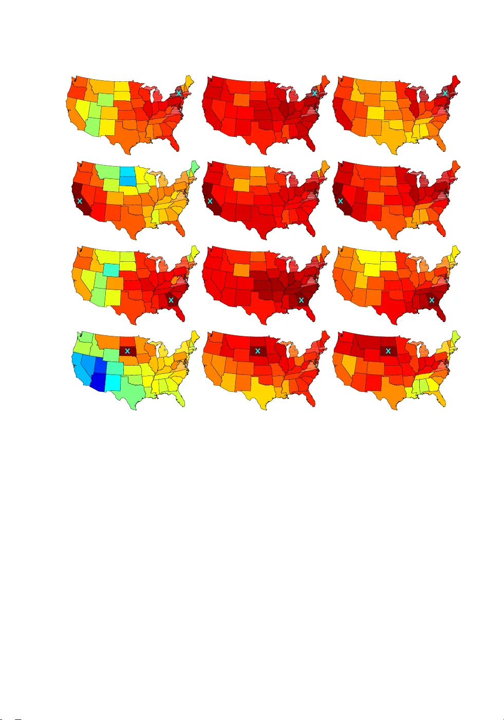
Ba yes ian Nonparametric Co v ariance Regressio n Emily Fo x Duke Univ ersity , Durham, NC USA. Da vid Dunson Duke Univ ersity , Durham, NC USA. Summary . Althou gh there is a rich literature on methods f or allowing the v ariance in a univari- ate regression model to v ar y with pre dictors, time and othe r factors , rela tively lit tle has been done in the multiv ari ate case. Our focus is on dev elop ing a class of nonpa rametric co variance regression models, which al low an un known p × p cov ari ance matr ix to change ﬂexibly with predicto rs. The pr oposed mode ling framework i nduces a prior o n a collection of cov ariance matrices ind ex ed by pre dictors th rough p rior s for p redictor-d epend ent load ings matr ices in a factor model. In par ti cular , the predictor-d epen dent loadi ngs are character ized as a sparse combinati on of a col lection of un known diction ar y functio ns (e.g, Gaussian process random function s). The induced co variance is then a regul arized quad ratic function of these dictionar y element s. Our pro posed framew or k leads to a hi ghly-ﬂexible, but computat ional ly tractable formulation with simple conjuga te posterio r updates that can readily handle missing data. The- oretical prop er ti es are d iscussed and the me thods are illustrated throug h simulation s stu dies and an applicat ion to the Googl e Flu T rends data. Keywor ds: co v ariance estimation; Gaussian proces s; heteroscedastic regression; nonparametric Bay es; stochastic pro cess. 1. Introduction Spurred by the increa sing pr ev a lence of high-dimensio na l datasets and the co mputational capacity to analyze them, capturing heteroscedas ticit y in multiv ariate pro cesses has be come a g r owing focus in ma ny applied domains. F or exa mple, within the ﬁeld of ﬁna nc ia l time series modeling , ca pturing the time-v a r ying volatility and c o-vola tility of a co lle ction of r isky assets is k ey in devising a p ortfolio management scheme. Likewise, the s pa tial statistics communit y is often faced with multiv ariate mea surements (e.g., temper ature, pr ecipitation, etc.) recorded at a lar ge collection o f lo cations, necessitating metho dolog y to mo de l the strong spatial (and spatio- tempo ral) v ar iations in correlatio ns. More generally , imagine that one has some arbitrary , p otentially m ultiv ar iate pr edictor space X and a co llection of m ultiv a riate r esp onse vectors y . The problem of mean re gressio n (i.e., µ ( x ) = E ( y | x )) has bee n well studied in b oth the univ ariate a nd multiv aria te settings . Although there is a rich literature o n methods for allowing the v ar iance in a univ ariate r e g ressio n mo del to v ary with predictors, there is a dear th of methodo lo gies for the general case of multiv ariate cov aria nce regres s ion (i.e., Σ( x ) = cov( y | x )). The cov a r iance matrix capture s k ey cor relations b etw een the elements of the r esp onse v ector, and the typical a ssumption of a homosceda stic mo del can have signiﬁca nt impact on inferences. Historically , the problem of multiv ariate cov a riance regr ession ha s typically be e n ad- dressed by standard regressio n op er ations on the unconstr ained elements o f the lo g or 2 Fo x and Dunson Cholesky decomp osition of the cov a riance (or pr ecision) matrix. F or example, Pourahmadi [ 1999 ] prop ose s to mo del elements of chol (Σ( x ) − 1 ) as a linear function o f the predictor s. The weigh ts asso cia ted with the i th row hav e a nice interpretation in terms of the co n- ditional distr ibution of y i given y 1 , y 2 , . . . , y i − 1 ; ho wev er, the model is not inv ar iant to per mutations of the elements o f y which is pro blematic in applications where there do es not exist a natura l or de r ing. Alternativ ely , Chiu e t al. [ 1 996 ] consider mo deling e a ch elemen t of log (Σ( x )) as a linear function of the pr e dic to r. An issue with this formulation is in the int erpretability of the mo del: a submatrix of Σ( x ) do e s not necessar ily coincide with a sub- matrix o f the ma trix loga rithm. Additionally , b oth the mo dels of Pourahmadi [ 1999 ] and Chiu et a l. [ 1996 ] involv e a large num b er of pa rameters (sp eciﬁcally , d × p ( p + 1) / 2 assuming x ∈ ℜ d .) More recently , Hoﬀ and Niu [ 201 0 ] prop os e a cov ar ia nce r egressio n mo del in which Σ( x ) = A + B xx ′ B ′ with A po sitive deﬁnite and B rea l. This mo del has interpretable parameters and may b e equated with a latent facto r mo del, leading to computational ad- v antages. How ev er, the mo del still has key limitations in (i) scaling to la r ge p doma ins, and (ii) ﬂe x ibilit y based o n the pa rametric a pproach. Speciﬁcally , the mo del restricts the diﬀerence b etw een Σ( x ) and the ba seline ma trix A to b e rank 1. Higher rank mo dels can be consider ed via extensions such as Σ( x ) = A + B xx ′ B ′ + C xx ′ C ′ , but this drama tically increases the par a meterization and requires deﬁnition o f the maximal r ank diﬀerence. F or volatility mo deling where the cov ariate spa ce is typically taken to b e discrete time, heteroscedas ticit y ha s classica lly b een captured via either v ar ia nts of AR CH [ Eng le , 2002 ] or sto chastic volatilit y mo dels [ Harvey et al. , 1994 ]. The former directly sp eciﬁes the volatilit y matrix as a linear combination o f lagged volatilities and squa r ed r eturns, which suﬀer s fr o m curse of dimensionality , and is typically limited to datasets with 5 or fewer dimensions. Alternatively , multiv ariate sto chastic volatility mo dels assume Σ( t ) = A Γ( t ) A ′ , with A rea l, Γ( t ) = diag(exp h 1 t , . . . , exp h pt ), and h it independent autoreg r essive pro cess es. See Chib et al. [ 2009 ] for a survey of s uch appro aches. Mo re recently , a num ber o f pap ers hav e examined inducing cov ariance pro cesse s through v ariants of a Wishart pr o cess. Philip ov and Glickman [ 200 6a ] take Σ( t ) − 1 | Σ( t − 1) ∼ W ( n, S t − 1 ) with S t − 1 = 1 /n ( A 1 / 2 )(Σ( t − 1) − 1 ) ν ( A 1 / 2 ) ′ † . Alter natively , a conditionally non-c entr al Wishart distribution is induced on the precision matrix in Gour i´ eroux et al. [ 200 9 ] by taking Σ( t ) = P p k =1 x kt x ′ kt , with each x k independently a ﬁrst o rder Ga us sian autor egressive pro cess. Key limitations of these t yp es of Wisha rt pro cesses are that p os terior c o mputations are ex tremely challenging, theory is la cking (e.g., simple descriptions o f marginal distributions), and s ingle parameter s (e.g., n and ν ) control the inter- and intra-tempora l cov aria nce relationships. Prado a nd W est [ 2010 ] review a lternative mo dels o f time-v a r ying cov ariance matrices for dyna mic linear mo dels via dis counting metho ds that main tain conjugacy . Central to a ll of the cited volatilit y mo dels is the a ssumption of Markov dynamics, limiting the a bility to capture long- range dependenc ie s and often lea ding to spiky tra jectories . Additionally , these metho ds assume a regula r gr id of obs erv ations that cannot easily accommo date missing v alues. Within the spatia l statistics c ommunit y , the term Wishart pr o c ess is t ypically used to sp ecify a diﬀer e nt fo rmulation than those descr ib ed herein for volatility mo deling . Specif- ically , letting Σ( s ) denote the cov ar iance of a p -dimensional obser v ation a t geogr aphic lo- cation s ∈ R 2 , Gelfand et al. [ 200 4 ] assume that Σ( s ) = A ( s ) A ( s ) ′ + Σ 0 with Σ 0 diagonal and T ( s ) = A ( s ) A ( s ) ′ following a matric-variate W ishart pr o c ess . This Wishart pro cess is such that T ( s ) − 1 = Θ ξ ( s ) ξ ( s ) ′ Θ ′ with ξ ℓj ∼ GP(0 , c j ) indep endently for ea ch ℓ, j and † Extending to higher dimensions, Philip ov and Glic kman [ 2006b ] apply this mo del to th e cov ari- ance of a low er-dimensional latent factor in a standard laten t factor mo del. Bay esian Nonparametri c Cov ar iance Regression 3 Θ typically taken to b e diago na l. The induced distributio n on T ( s ) is then marginally in- verse Wishart ‡ . Posterior co mputations in this mo del r ely on Metrop olis-Hastings prop osa ls that do not s cale well to dimensions p la rger than 2- 3 and cannot na turally acco mmo date missing data. In terms of spatio-temp oral pr o cesses, Lop es e t a l. [ 2 008 ] build upon a stan- dard dynamic factor model to dev elop no nseparable and nonstationa ry space - time mo dels. Spec iﬁc a lly , the vector y t of univ ariate observ ations y st at spatial lo cations s is mo deled as y t = µ t + β f t + ǫ t with the comp onents of the la tent fa ctors f t independently evolving according to a ﬁrst-or der autor egressive pro ces s a nd columns of the factor loa dings matrix β indep endently drawn fro m Ma rko v r andom ﬁelds. Key a ssumptions o f this formulation are that the obser v a tio ns evolv e in discrete time on a reg ular gr id, and that the dyna mics of the spa tio -temp oral pro c e ss are c a ptured by indep endent random walks o n the c o mp o nents of the latent factors . In this pap er, we pr esent a Bayesian nonpara metric a pproach to multiv ar ia te cov ar ia nce regres s ion that allows the cov aria nce matrix to change ﬂexibly with predictor s a nd rea dily scales to high-dimensio na l data sets. The prop osed mo deling framework induces a prior on a c o llection o f cov ariance ma trices Σ X = { Σ( x ) , x ∈ X } thro ugh speciﬁca tion of a prior on a predictor -dep endent latent factor mo del. In particular , the predictor- depe ndent loadings are characterized as a spar se combination of a collectio n of unknown dictiona ry functions (e.g, Gaussian pro cess random functions). The induced cov ar iance is then a regular iz ed qua dratic function of these dictionar y elements. Th e prop osed metho do logy has numerous adv an tages over previous approa ches. By employing collectio ns o f contin uous random functions, we allow for an irr e g ular grid of obser v a tions. Similarly , we can easily cop e with missing data within our framework without relying on imputing the missing v alue s . Another fundamental prop erty of the prop os ed methodo logy is the fact that our combined use o f a shrink age pr ior with a latent factor mo del ena bles us (in theory) to handle high-dimensional da tasets (e.g., on the order of hundreds of dimensio ns) in the pr esence of a limited nu mber of observ ations. E ssential in b eing able to cop e with such larg e datasets in practice is the fact that our co mputations are tractable, ba sed on simple conjugate p os terior upda tes. Finally , w e are able to state theoretical prop er ties of o ur prop osed prior, such as large s uppo rt. The pap er is org anized as follows. In Section 2 , we descr ibe our prop osed Bay esian nonparametric cov ariance r egressio n mo del in addition to ana lyzing the theor etical pr op- erties of the mo del. Section 3 details the Gibbs sampling steps inv olved in our p os ter ior computations. Finally , a num ber o f simu lation studies a re examined in Section 4 , with an application to the Go ogle T rends ﬂu dataset pr esented in Sec tio n 5 . 2. Cov ariance Regression Priors 2.1. Notation and Motiv ation Let Σ( x ) deno te the p × p cov ar iance matrix at “lo ca tion” x ∈ X . In general, x is an arbitrar y , pos sibly multiv aria te predictor v alue. In dynamical mo deling, x may s imply represent a discrete time index (i.e., X = { 1 , . . . , T } ) or, in spatial mo deling, a g eogra phical lo cation (i.e., X = ℜ 2 ). Another simple, tractable case is when x repr esents an o r dered ‡ More generally , Gelfand et al. [ 2004 ] dev elop a sp atial coregionali zation mo del such that co v( y ( s 1 ) , y ( s 2 )) = ρ ( s 1 − s 2 ) A ( s 1 ) A ( s 2 ) ′ + Σ 0 (i.e., a mo del with spatial dep end encies arising in b oth the cov ariance and cr oss cov ariance). 4 Fo x and Dunson categoric al pr edictor (i.e., X = { 1 , . . . , N } ). W e se e k a prior for Σ X = { Σ( x ) , x ∈ X } , the collection of cov aria nce matrices ov er the space of predictor v alues. Letting Σ X ∼ Π Σ our g oal is to choo s e a prior Π Σ for the collection of cov ariance matrices that ha s lar ge supp or t and leads to go o d pe r formance in la rge p settings. By “go o d” we mean accurate estimation in small samples, taking a dv a nt age of shrink age priors and eﬃcient computation that scales well as p increa s es. W e initially fo c us on the r elatively simple setting in which y i ∼ N p ( µ ( x i ) , Σ( x i )) (1) independently for each i . Suc h a formulation could be extended to settings in which data are collec ted at r ep e ated times for diﬀerent sub jects, a s in m ultiv a riate longitudinal data analysis, by embedding the pro p osed mo del within a hiera rchical framework. See Section 6 for a discussion. 2.2. Proposed Latent F actor Model In large p settings, mo deling a p × p cov ar ia nce matrix Σ( x ) over an arbitrary predictor space X represents a n enormous dimensional regres s ion pr oblem; we aim to r educe dimensional- it y fo r tra ctability in building a ﬂexible nonpar ametric mo del for the predictor -dep endent cov ariances . A po pular a ppr oach for co ping with such high dimensional (non- pr edictor- depe ndent) cov ar ia nce matrices Σ in the presence of limited data is to a ssume that the cov ariance has a decomp ositio n as ΛΛ ′ + Σ 0 where Λ is a p × k factor loadings matrix with k << p and Σ 0 is a p × p diagonal matrix with non-nega tive entries. T o build in predictor depe ndence , w e as sume a decomp osition Σ( x ) = Λ( x )Λ( x ) ′ + Σ 0 , (2) where Λ( x ) is a p × k factor lo adings ma trix that is indexed by predictors x and where Σ 0 = diag( σ 2 1 , . . . , σ 2 p ). Assuming initia lly for simplicity that µ ( x ) = 0 , such a decomp os ition is induced by ma rginalizing out a set of latent factors η i from the fo llowing latent factor mo del: y i = Λ( x i ) η i + ǫ i η i ∼ N k (0 , I k ) , ǫ i ∼ N p (0 , Σ 0 ) . (3) Here, x i = ( x i 1 , . . . , x iq ) ′ is the predictor asso cia ted with the i th observ ation y i . Despite the dimensionality reduction intro duced by the latent factor mo del of E q. ( 3 ), mo deling a p × k dimensio nal pr edictor-dep endent factor loadings matrix Λ( x ) still represents a signiﬁcant challenge for la rge p domains. T o further reduce dimensionalit y , and fo llowing the strategy of building a ﬂexible high-dimensional model fro m s imple low-dimensional pieces, we ass ume that ea ch element of Λ( x ) is a linear combination o f a muc h smaller nu mber of unknown dictiona r y functions ξ ℓk : X → ℜ . That is, we prop o se to let Λ( x i ) = Θ ξ ( x i ) , (4) where Θ ∈ ℜ p × L is the matrix of co eﬃcients relating the predicto r-dep endent factor loading s matrix to the set of dictionary functions comprising the L × k dimensio na l ma trix ξ ( x ). Typically , k << p and L << p . Since w e ca n write [Λ( · )] r s = L X ℓ =1 θ r ℓ ξ ℓs ( · ) , (5) Bay esian Nonparametri c Cov ar iance Regression 5 we see that the weigh ted sum of the s th column of dictionar y functions ξ · s ( · ), with weights sp eciﬁed by the r th row of Θ, character iz es the impact of the s th latent factor o n y ir , the r th comp onent of the resp onse at predictor lo cation x i . By characterizing the elemen ts of Λ( x i ) as a linear combination of thes e ﬂexible dictionary functions, we obta in a highly-ﬂexible but co mputationally tractable formulation. In mar g inalizing out the latent facto rs, we now o btain the following induced cov ariance structure cov ( y i | x i = x ) = Σ( x ) = Θ ξ ( x ) ξ ( x ) ′ Θ ′ + Σ 0 . (6) Note that the ab ov e decomp osition of Σ( x ) is not unique and there a re actually inﬁnitely many such e q uiv a le nt decomp ositio ns. F or exa mple, ta ke Θ 1 = c Θ and ξ 1 ( · ) = (1 /c ) ξ ( · ). Alternatively , consider ξ 1 ( · ) = ξ ( · ) P for any orthogo nal matr ix P or Θ 1 = [Θ 0 p × d ] and ξ 1 = [ ξ ; ξ 0 ] for any d × k matrix of dictio na ry functions ξ 0 . One ca n als o increase the dimen- sion of the latent factors and take ξ 1 = [ ξ 0 L × d ]. In standard (non-predictor -dep endent) latent facto r modeling , a common appr oach to ens ure identiﬁabilit y is to cons train the factor lo adings matr ix to b e block low er triangula r with strictly p o sitive diago nal ele- men ts [ Gewek e a nd Zhou , 1996 ], though such a constraint induces order dep endence among the res p o nses [ Aguilar and W est , 20 00 , W est , 200 3 , Lop es and W est , 2004 , Car v a lho et a l. , 2008 ]. Howev er, for tasks suc h as inference on the cov aria nce matr ix and prediction, iden- tiﬁabilit y of a unique decomp ositio n is not necessary . Thus, we do not restrict ourse lves to a unique decomp osition of Σ( x ), allowing us to deﬁne priors with b etter computational prop erties. Although w e are not interested in ident ifying a unique decomp o sition o f Σ( x ), we a re int erested in characterizing the class of cov aria nce regressio ns Σ( x ) that can b e decomp osed as in Eq. ( 6 ). Lemma 2.1 sta tes that for L and k suﬃciently larg e, a ny cov aria nce regr e ssion has s uch a deco mpo sition. F or L, k ≥ p , let X ξ denote the space of all L × k dimensional matrices o f arbitra rily complex dictiona ry functions mapping from X → ℜ , X Σ 0 be the space of all p × p diagona l matrices with non-neg ative en tries, and X Θ be the spa ce of all p × L dimensional ma trices Θ such that ΘΘ ′ has ﬁnite elements. Lemma 2.1 . Given a symmetric p ositive semideﬁnite matrix Σ( x ) ≻ 0 , ∀ x ∈ X , ther e exists { ξ ( · ) , Θ , Σ 0 } ∈ X ξ ⊗ X Θ ⊗ X Σ 0 such that Σ( x ) = Θ ξ ( x ) ξ ( x ) ′ Θ ′ + Σ 0 , ∀ x ∈ X . (7) Proof. Assume without loss of gener ality that Σ 0 = 0 p × p and take k , L ≥ p . Consider Θ = [ I p 0 p × L − p ] ξ ( x ) =  chol (Σ( x )) 0 p × k − p 0 L − p × p 0 L − p × k − p  . (8) Then, Σ( x ) = Θ ξ ( x ) ξ ( x ) ′ Θ ′ , ∀ x ∈ X . Now that we hav e esta blished that there exist decomp os itions o f Σ( x ) into the form sp eciﬁed by Equation ( 6 ), the questio n is whether we c an sp ecify a prior on the elements ξ ( · ), Θ, and Σ 0 that provides lar ge supp ort on suc h deco mpo sitions. This is explored in Section 2.3 . 6 Fo x and Dunson In order to g eneralize the model to also allow the mean µ ( x ) to v ar y ﬂexibly with predictors, we ca n follow a nonparametric laten t factor regr e ssion approa ch and le t η i = ψ ( x i ) + ν i , ν i ∼ N k (0 , I k ) , (9) where ψ ( x i ) = [ ψ 1 ( x i ) , . . . , ψ k ( x i )] ′ , and ψ j : X → ℜ is an unkno wn function r elating the predictors to the mean of the j th factor, for j = 1 , . . . , k . These ψ j ( · ) functions can be mo deled in a rela ted manner to the ξ ℓk ( · ) functions de s crib ed ab ov e. The induced mean of y i conditionally on x i = x and mar ginalizing out the la tent factors is then µ ( x ) = Θ ξ ( x ) ψ ( x ). F or simplicity , how ever, we fo cus our discussions on the case where µ ( x ) = 0. 2.3. Prior Speciﬁcation W orking within a Bay esian framework, we place indep endent pr iors on ξ ( · ), Θ , and Σ 0 in Eq. ( 6 ) to induce a prio r on Σ X . Le t Π ξ , Π Θ , and Π Σ 0 denote each of these indep endent priors, r esp ectively . Recall that Π Σ denotes the induced prior o n Σ X . Aiming to capture cov ar iances that v ary co ntin uously over X co m bined with the goal of maintaining simple co mputations for inference , we sp ecify the dictionary functions as ξ ℓk ( · ) ∼ GP (0 , c ) (10) independently for all ℓ, k , with c a square d exp onential correlation function having c ( ξ , ξ ′ ) = exp( − κ || ξ − ξ ′ || 2 2 ). T o cop e with the fact that the num be r of la tent dictionar y functions is a mo del c hoice we are required to make, we seek a prior Π Θ that fav ors many v alues of Θ b eing clos e to zero so that we may choose L la rger tha n the exp ected num b er of dictionary functions (also controlled b y the latent factor dimension k ). As prop os e d in Bhattacharya and Dunson [ 2010 ], w e use the following shrink ag e prior : θ j ℓ | φ j ℓ , τ ℓ ∼ N ( 0 , φ − 1 j ℓ τ − 1 ℓ ) φ j ℓ ∼ Ga(3 / 2 , 3 / 2 ) δ 1 ∼ Ga ( a 1 , 1) , δ h ∼ Ga( a 2 , 1) , h ≥ 2 , τ ℓ = ℓ Y h =1 δ h . (11) Cho osing a 2 > 1 implies that δ h is greater than 1 in exp ectation so that τ ℓ tends sto chas- tically tow ards inﬁnit y as ℓ go es to inﬁnity , thus shrinking the elements θ j ℓ tow ard zero increasingly as ℓ grows. The φ j ℓ precision par ameters allow for ﬂexibility in how the ele- men ts of Θ are shrunk tow ards zero by incor p orating lo cal shr ink age sp eciﬁc to ea ch elemen t of Θ, while τ ℓ provides a global column-wis e shrink age factor. Finally , w e sp ecify Π Σ 0 via the usual in verse gamma prio rs on the dia gonal ele ments of Σ 0 . That is, σ − 2 j ∼ Ga ( a σ , b σ ) (12) independently for each j = 1 , . . . , p . 2.4. Theoretical Proper ties In this section, we explore the theoretical prop erties o f the pr op osed Bayesian nonparametric cov ariance r egress ion mo del. In particular, we fo cus on the supp ort of the induced prior Bay esian Nonparametri c Cov ar iance Regression 7 Π Σ based on the prio rs Π ξ , Π Θ , and Π Σ 0 deﬁned in Sectio n 2.3 . Larg e supp ort implies that the prio r can g enerate cov aria nce regr essions that ar e arbitra rily clo se to any function { Σ( x ) , x ∈ X } in a lar g e cla ss. Such a supp or t pro p e r ty is the deﬁning featur e of a Bayesian nonparametric appr oach and ca nnot simply b e assumed. Often, se e mingly ﬂexible mo dels can have quite restric ted s uppo rt due to hidden cons tr aints in the mo del and not to real prior knowledge that certain v alues are implausible. Although we have chosen a sp eciﬁc for m for a shrink a ge prio r Π Θ , we aim to make our sta temen t o f pr io r supp or t as g eneral a s p o ssible and th us simply assume that Π Θ satisﬁes a set of t wo conditions given by Assumption 2.1 and Assumption 2.2 . In Lemma 2.2 , we show that the Π Θ sp eciﬁed in Eq. ( 11 ) satisﬁes these assumptions. The pro o fs as so ciated with the theoretical sta tements ma de in this section can b e found in the App endix. Assumption 2.1. Π Θ is such that P ℓ E [ | θ j ℓ | ] < ∞ . This pr op erty ensur es that the prior on t he r ows of Θ shrinks the elements towar ds zer o fast en ou gh as ℓ → ∞ . Assumption 2.2. Π Θ is such t hat Π Θ ( r ank (Θ) = p ) > 0 . Tha t is, ther e is p ositive prior pr ob ability of Θ b eing ful l r ank. The following theo rem s hows that, for k ≥ p and as L → ∞ , the induced prior Π Σ places po sitive proba bilit y o n the space of all cov a riance functions Σ ∗ ( x ) that are contin uous on X . Theorem 2.1. L et Π Σ denote the induc e d prior on { Σ( x ) , x ∈ X } b ase d on the sp e ciﬁe d prior Π ξ ⊗ Π Θ ⊗ Π Σ 0 on X ξ ⊗ X Θ ⊗ X Σ 0 . Assuming X c omp act, for al l c ontinuous Σ ∗ ( x ) and for al l ǫ > 0 , Π Σ  sup x ∈X || Σ( x ) − Σ ∗ ( x ) || 2 < ǫ  > 0 . (13) Int uitively , the supp ort on co ntin uous cov aria nce functions Σ ∗ ( x ) aris e s from the contin uit y of the Gauss ia n pro cess dictionary functions. Ho w ever, s ince we a re mixing ov er inﬁnitely many such dictionary functions, we need the mixing weigh ts sp eciﬁed by Θ to tend towards zero, and to do so “fast enough”—this is where Assumption 2.1 b ecomes imp o rtant. See Theorem 2 .2 . The pro o f of Theorem 2.1 relies on the large suppo rt of Π Σ at a ny p oint x 0 ∈ X . Since each ξ ℓk ( x 0 ) is indep endently Ga ussian distributed (based on pro per ties of the Gaussian pro c e ss prior), ξ ( x 0 ) ξ ( x 0 ) ′ is Wishart distributed. Co nditioned on Θ, Θ ξ ( x 0 ) ξ ( x 0 ) ′ Θ ′ is also Wishart distributed. More generally , for ﬁxed Θ, Θ ξ ( x ) ξ ( x ) ′ Θ ′ follows the matric-v ariate Wisha rt pro ce s s of Gelfand et al. [ 200 4 ]. Co mb ining the la rge suppo rt of the Wishart distr ibution with that of the gamma distribution o n the inv erse elements of Σ 0 provides the des ired lar ge supp ort of the induced prior Π Σ at ea ch predictor lo cation x 0 . Theorem 2.2. F or every ﬁnite k and L → ∞ (or L ﬁnite), Λ( · ) = Θ ξ ( · ) is almost sur ely c ontinuous on X . Lemma 2.2 sp eciﬁes the conditio ns und er which the prior Π Θ sp eciﬁed in Eq. ( 1 1 ) satisﬁes Assumption 2.1 , which provides a suﬃcient condition used in the pr o of of pr ior suppo rt. 8 Fo x and Dunson Lemma 2.2 . Base d on the prior sp e ciﬁe d in Eq. ( 11 ) and cho osing a 2 > 2 , A ssump- tion 2.1 is satisﬁe d. That is, P ℓ E [ | θ j ℓ | ] < ∞ . It is a lso o f int erest to analyze the moments asso cia ted with the prop osed prior . As detailed in the App endix, the ﬁrst moment can b e derived ba sed on the implied inv erse gamma prior on the σ 2 j combined with the fact that Θ ξ ( x ) ξ ( x ) ′ Θ ′ is marginally Wishart distributed at every lo ca tion x , with the prio r on Θ speciﬁed in E quation ( 11 ). Lemma 2.3 . L et µ σ denote the me an of σ 2 j , j = 1 , . . . , p . Then, E [Σ( x )] = diag k X ℓ φ − 1 1 ℓ τ − 1 ℓ + µ σ , . . . , k X ℓ φ − 1 pℓ τ − 1 ℓ + µ σ ! . (14) Since our goal is to dev elop a cov a riance regr ession mo del, it is natural to consider the correla tion induced b etw een an elemen t of the co v ariance matrix at diﬀerent predicto r lo cations x and x ′ . Lemma 2.4 . L et σ 2 σ denote the varianc e of σ 2 j , j = 1 , . . . , p . Then, c ov ( Σ ij ( x ) , Σ ij ( x ′ )) = ( k c ( x, x ′ )  5 P ℓ φ − 2 iℓ τ − 2 ℓ + ( P ℓ φ − 1 iℓ τ − 1 ℓ ) 2  + σ 2 σ i = j, k c ( x, x ′ )  P ℓ φ − 1 iℓ φ − 1 j ℓ τ − 2 ℓ + P ℓ φ − 1 iℓ τ − 1 ℓ P ℓ ′ φ − 1 j ℓ ′ τ − 1 ℓ ′  i 6 = j. (15) F or any t wo elements Σ ij ( x ) and Σ uv ( x ′ ) with i 6 = u or j 6 = v , c ov ( Σ ij ( x ) , Σ uv ( x ′ )) = 0 . (16) W e ca n thus conclude that in the limit as the distance b etw een the predictor s tends tow ards inﬁnit y , the correla tion decays at a ra te deﬁned by the Gaussia n pr o cess kernel c ( x, x ′ ) w ith a limit: lim || x − x ′ ||→∞ cov (Σ ij ( x ) , Σ uv ( x ′ )) =  σ 2 σ i = j = u = v , 0 otherwise . (17) It is p erha ps counterint uitive that the co rrelatio n b e tw een Σ ii ( x ) and Σ ii ( x ′ ) do es not g o to zero as the dista nc e b etw een the pre dictors x and x ′ tends to inﬁnity . How ever, although the cor relation b etw een ξ ( x ) and ξ ( x ′ ) go es to zer o, the diagonal matrix Σ 0 do es no t dep end on x or x ′ and thus r etains the correlatio n betw een the diagonal elemen ts o f Σ( x ) and Σ( x ′ ). Equation ( 15 ) implies that the auto co rrelatio n AC F ( x ) = co rr(Σ ij (0) , Σ ij ( x )) is simply sp eciﬁed by c (0 , x ). When we cho ose a Gaussian pro cess k ernel c ( x, x ′ ) = exp( − κ || x − x ′ || 2 2 ), we have AC F ( x ) = exp( − κ || x || 2 2 ) . (18) Thu s, we see that the length-sc ale parameter κ dir ectly determines the sha pe of the auto - correla tion function. Finally , one can analy ze the stationarity pro p erties of the pr op osed cov a riance regressio n prior. Bay esian Nonparametri c Cov ar iance Regression 9 Lemma 2.5 . Our pr op ose d c ovarianc e r e gr ession mo del deﬁnes a ﬁrst- or der stationary pr o c ess in that Π Σ (Σ( x )) = Π Σ (Σ( x ′ )) , ∀ x, x ′ ∈ X . F u rthermor e, the pr o c ess is wide s ense stationary: c ov (Σ ij ( x ) , Σ uv ( x ′ )) solely dep ends up on || x − x ′ || . Proof. Th e ﬁrst -or der stat ionarity fol lows imme diately fr om the stationarity of t he Gaussian pr o c ess dictionary elements ξ ℓk ( · ) and r e c al ling that Σ( x ) = Θ ξ ( x ) ξ ( x ) ′ Θ ′ + Σ 0 . Assuming a Gaussian pr o c ess kernel c ( x, x ′ ) t hat solely dep ends up on the distanc e b etwe en x and x ′ (as in Se ction 2.3 ), Equations ( 15 ) - ( 16 ) imply that the deﬁne d pr o c ess is wide sense stationary. 3. P osterior Computation 3.1. Gibbs Sampl ing with a Fixed T runcation Lev el Based on a ﬁxed truncation lev el L ∗ and a latent factor dimens io n k ∗ , we prop os e a Gibbs sampler for p oster ior computatio n. The deriv a tion o f Step 1 is provided in the App endix. Step 1 Up date ea ch dictiona ry function ξ ℓm ( · ) from the conditiona l p oster ior given { y i } , Θ, { η i } , Σ 0 . W e ca n rewrite the obser v a tio n mo del for the j th comp onent of the i th resp onse as y ij = k ∗ X m =1 η im L ∗ X ℓ =1 θ j ℓ ξ ℓm ( x i ) + ǫ ij . (19) Conditioning on ξ ( · ) − ℓm = { ξ r s ( · ) , r 6 = ℓ, s 6 = m } , our Gauss ian pr o cess prio r on the dictio- nary functions implies the follo wing conditional p oster ior      ξ ℓm ( x 1 ) ξ ℓm ( x 2 ) . . . ξ ℓm ( x n )      | { y i } , Θ , η , ξ ( · ) − ℓm , Σ 0 ∼ N n    ˜ Σ ξ    η 1 m P p j =1 θ j ℓ σ − 2 j ˜ y 1 j . . . η nm P p j =1 θ j ℓ σ − 2 j ˜ y nj    , ˜ Σ ξ    , (20) where ˜ y ij = y ij − P ( r,s ) 6 =( ℓ,m ) θ j r ξ r s ( x i ) a nd, taking K to be the Gaussian pro cess cov ariance matrix with K ij = c ( x i , x j ), ˜ Σ − 1 ξ = K − 1 + diag   η 2 1 m p X j =1 θ 2 j ℓ σ − 2 j , . . . , η 2 nm p X j =1 θ 2 j ℓ σ − 2 j   . (21) Step 2 Next we sample e ach la tent fa ctor η i given y i , ξ ( · ), Θ, Σ 0 . Recalling Eq. ( 3 ) and the fact that η i ∼ N k ∗ (0 , I k ∗ ), η i | y i , Θ , ξ ( x i ) , Σ 0 ∼ N k ∗   I + ξ ( x i ) ′ Θ ′ Σ − 1 0 Θ ξ ( x i )  − 1 ξ ( x i ) ′ Θ ′ Σ − 1 0 y i ,  I + ξ ( x i ) ′ Θ ′ Σ − 1 0 Θ ξ ( x i )  − 1  . (22) 10 F ox and Dun son Step 3 Let θ j · =  θ j 1 . . . θ j L ∗  . Recalling the Ga( a σ , b σ ) prior o n each prec ision pa - rameter σ − 2 j asso ciated with the diagona l noise cov ar iance matrix Σ 0 , standard co njuga te po sterior analysis yields the po sterior σ − 2 j | { y i } , Θ , η , ξ ( · ) ∼ Ga a σ + n 2 , b σ + 1 2 n X i =1 ( y ij − θ j · ξ ( x i ) η i ) 2 ! . (23) Step 4 Conditioned on the h yp erpara meters φ and τ , the Gaussian prior on the elements o f Θ spe c iﬁed in Eq. ( 11 ) combined with the likelihoo d deﬁned by E q. ( 3 ) imply the following po sterior for each row of Θ: θ j · | { y i } , η , ξ ( · ) , φ, τ ∼ N L ∗    ˜ Σ θ ˜ η ′ σ − 2 j    y 1 j . . . y nj    , ˜ Σ θ    , (24) where ˜ η ′ =  ξ ( x 1 ) η 1 ξ ( x 2 ) η 2 . . . ξ ( x n ) η n  and ˜ Σ − 1 θ = σ − 2 j ˜ η ′ ˜ η + diag( φ j 1 τ 1 , . . . , φ j L ∗ τ L ∗ ) . (25) Step 5 Examining E q. ( 11 ) and using standa rd conjugate analysis results in the follo wing po sterior for each lo cal shrink age hyperpara meter φ j ℓ given θ j ℓ and τ ℓ : φ j ℓ | θ j ℓ , τ ℓ ∼ Ga 2 , 3 + τ ℓ θ 2 j ℓ 2 ! . (26) Step 6 As in Bhattacharya and Dunson [ 201 0 ], the g lobal shrink age hyper pa rameters are upda ted as δ 1 | Θ , τ ( − 1) ∼ Ga   a 1 + pL ∗ 2 , 1 + 1 2 L ∗ X ℓ =1 τ ( − 1) ℓ p X j =1 φ j ℓ θ 2 j ℓ   δ h | Θ , τ ( − h ) ∼ Ga   a 2 + p ( L ∗ − h + 1) 2 , 1 + 1 2 L ∗ X ℓ =1 τ ( − h ) ℓ p X j =1 φ j ℓ θ 2 j ℓ   , (27) where τ ( − h ) ℓ = Q ℓ t =1 ,t 6 = h δ t for h = 1 , . . . , p . 3.2. Incor porating nonpar ametric mean µ ( x ) If one wishes to inco rp orate a latent factor r egressio n mo del such as in Eq. ( 9 ) to induce a predictor- dep endent mean µ ( x ), the MCMC sampling is mo diﬁed as follows. Steps 1, 3, 4, 5, and 6 are exactly as b efor e. Now, how ever, the sampling of η i of Step 2 is repla ced by a blo ck sampling of ψ ( x i ) and ν i . Speciﬁca lly , let Ω i = Θ ξ ( x i ). W e can rewrite the observ ation mo del a s y i = Ω i ψ ( x i ) + Ω i ν i + ǫ i . Marg inalizing out ν i , y i = Ω i ψ ( x i ) + ω i Bay esian Nonparametri c Cov arian ce Regression 11 with ω i ∼ N (0 , ˜ Σ i , Ω i Ω ′ i + Σ 0 ). Assuming no nparametric mean vector co mpo nents ψ ℓ ( · ) ∼ GP (0 , c ), the p osterio r of ψ ℓ ( · ) follows analogously to that of ξ ( · ) resulting in      ψ ℓ ( x 1 ) ψ ℓ ( x 2 ) . . . ψ ℓ ( x n )      | { y i } , ψ ( · ) − ℓ , Θ , η , ξ ( · ) , Σ 0 ∼ N n    ˜ Σ ψ    [Ω 1 ] ′ · ℓ ˜ Σ − 1 1 ˜ y − ℓ 1 . . . [Ω n ] ′ · ℓ ˜ Σ − 1 n ˜ y − ℓ n    , ˜ Σ ψ    , (28) where ˜ y − ℓ i = y i − P ( r 6 = ℓ ) [Ω i ] · r ψ r ( x i ). O nc e again taking K to b e the Ga ussian pro cess cov ariance matrix , ˜ Σ − 1 ξ = K − 1 + diag  [Ω 1 ] ′ · ℓ ˜ Σ − 1 1 [Ω 1 ] · ℓ , . . . , [Ω n ] ′ · ℓ ˜ Σ − 1 n [Ω n ] · ℓ  . (29) Conditioned on ψ ( x i ), we cons ider ˜ y i = y i − Ω i ψ ( x i ) = Ω i ν i + ǫ i . Then, using the fact that ν i ∼ N (0 , I k ∗ ), ν i | ˜ y i , ψ ( x i ) , Θ , ξ ( x i ) , Σ 0 ∼ N k ∗   I + ξ ( x i ) ′ Θ ′ Σ − 1 0 Θ ξ ( x i )  − 1 ξ ( x i ) ′ Θ ′ Σ − 1 0 ˜ y i ,  I + ξ ( x i ) ′ Θ ′ Σ − 1 0 Θ ξ ( x i )  − 1  . (30) 3.3. Hyper parameter Samplin g One can also co nsider sampling the Gaussia n pro cess length-scale hyperpa r ameter κ . Due to the linear-Ga ussianity of the pro p osed cov ariance regres s ion mo de l, we can analytically marginalize the latent Gaussia n pro cess random functions in consider ing the po s terior of κ . O nce again taking µ ( x ) = 0 for simplicity , our p osterior is ba sed on marg inalizing the Gaussian pro cess ra ndom vectors ξ ℓm = [ ξ ℓm ( x 1 ) . . . ξ ℓm ( x n )] ′ . Noting that  y ′ 1 y ′ 2 . . . y ′ n  ′ = X ℓm [diag( η · m ) ⊗ θ · ℓ ] ξ ℓm +  ǫ ′ 1 ǫ ′ 2 . . . ǫ ′ n  ′ , (31) and letting K κ denote the Gaus sian pro ce s s cov a riance matrix based o n a length-sca le κ ,      y 1 y 2 . . . y n      | κ, Θ , η , Σ 0 ∼ N np      X ℓ,m [diag( η · m ) ⊗ θ · ℓ ] K κ [diag( η · m ) ⊗ θ · ℓ ] ′ +      Σ 0 Σ 0 . . . Σ 0           . (32) W e ca n then Gibbs sample κ based on a ﬁxed g rid a nd prior p ( κ ) on this grid. Note, how ev er, that computatio n of the likeliho o d sp eciﬁed in Eq. ( 32 ) requir es ev aluation of an np -dimensional Gaussian for ea ch v a lue κ spe c iﬁe d in the gr id. F or lar ge p scenar ios, or when there ar e many o bserv ations y i , this may b e computationally infeasible. In such cases, a naive alterna tive is to iter ate b etw een sampling ξ ( · ) given K κ and K κ given ξ ( · ). How ev er, this ca n lead to extremely slow mixing. Alterna tively , one can consider emplo ying the recen t Ga us sian pro ces s hyper parameter slice sampler of Adams and Murray [ 201 1 ]. In general, bec a use o f the quadratic mixing over Gauss ian pr o cess dictionary elements, our mo del is relatively robust to the choice of the length-scale parameter and the computa- tional bur den imposed by sampling κ is typically unw arra nt ed. Instead, one can pre- s elect 12 F ox and Dun son T able 1. Computa tions requi red at each Gibbs sampling step. Gibbs Up date Computation Step 1 L ∗ × k ∗ draw s from an n dimensional Gaussian Step 2 n draw s from a k ∗ dimensional Gaussian Step 3 p dra ws from a gamma distribution Step 4 p dra ws from an L ∗ dimensional Gaussian Step 5 p × L ∗ draw s from a gamma distribution Step 6 L ∗ draw s from a gamma distribution a v alue for κ using a da ta -driven heuristic, which leads to a quas i-empirical Bayes appro ach. Recalling Equation ( 18 ), we hav e − log( AC F ( x )) = κ || x || 2 2 . (33) Thu s, if one can devise a pro c e dur e for estimating the auto co r relation function from the data, o ne ca n set κ a ccordingly . W e prop ose the following. 1. F or a set o f ev enly spaced kno ts x k ∈ X , compute the sample cov aria nce ˆ Σ( x k ) from a lo c al bin of data y k − k 0 : k + k 0 with k 0 > p/ 2. 2. Compute the Cho lesky decompo s ition C ( x k ) = chol ( ˆ Σ( x k )). 3. Fit a spline thr ough the elements of the computed C ( x k ). Denote the s pline ﬁt o f the Cholesky b y ˜ C ( x ) for ea ch x ∈ X 4. F or i = 1 , . . . , n , compute a p oint-b y-p oint estimate of Σ( x i ) from the splines: Σ( x i ) = ˜ C ( x i ) ˜ C ( x i ) ′ . 5. Compute the auto corr elation function o f ea ch elemen t Σ ij ( x ) o f this kernel-estimated Σ( x ). 6. According to Equation ( 33 ), choo se κ to b es t ﬁt the mo st correla ted Σ ij ( x ) (since les s correla ted co mpo nent s can b e captured via weigh tings of dictio nary elements with stronger correlation.) 3.4. Computational Considerations In choo sing a trunca tion level L ∗ and la tent factor dimension k ∗ , there ar e a num b er of computational considera tions. The Gibbs sa mpler o utlined in Sectio n 3.1 inv olv es a lar ge nu mber of s imu lations from Ga ussian distributio ns , each of which requires the inversion of an m - dimensional cov ariance matrix, with m the dimension of the Gauss ian. F or larg e m , this repres e nt s a large computationa l bur de n as the op er ation is, in gener al, O ( m 3 ). The computatio ns r e quired at each sta ge of the Gibbs sampler a re summar ized in T able 1 . F rom this table we s e e that dep ending on the n umber o f obse r v a tions n and the dimension of these obse rv ations p , v arious combinations of L ∗ and k ∗ lead to mo r e or less eﬃcient computations. In Bhattacharya and Dunso n [ 201 0 ], a metho d for adaptively choos ing the n umber of factors in a non- predictor dep endent latent factor mo del w as prop osed. One could directly apply s uch a metho dolo gy for ada ptively selecting L ∗ . T o handle the choice of k ∗ , one could consider a n augmen ted for mulation in which Λ( x ) = Θ ξ ( x )Γ , (34) Bay esian Nonparametri c Cov arian ce Regression 13 where Γ = diag( γ 1 , . . . , γ k ) is a diag onal matrix of par ameters that shr ink the columns o f ξ ( x ) tow ards zero. One ca n tak e these shrink age parameter s to be distributed as γ i ∼ N (0 , ω − 1 i ) , ω i = i Y h =1 ζ h ζ 1 ∼ Ga ( a 3 , 1) , ζ h ∼ Ga ( a 4 , 1) h = 2 , . . . , k . (35) F or a 4 > 1, such a mo del shrinks the γ i v alue s tow ards zero for lar ge indices i just as in the shr ink a g e pr ior o n Θ. The γ i close to zero provide insight int o redundant latent factor dimensions . Computations in this a ugmented mo del are a str aightforw ard ex tension of the Gibbs sampler presented in Section 3.1 . Bas ed o n the infer r ed v alues of the la tent γ i parameters , one can design an adaptive strateg y similar to that for L ∗ . Note that in Step 1, the n -dimensional inv erse cov ariance matrix ˜ Σ − 1 ξ which needs to be inv erted in order to sample ξ ℓm is a comp ositio n o f a diagona l matrix and an inv erse cov ariance matrix K − 1 that ha s entries that tend tow ards zero as || x i − x j || 2 bec omes large (i.e., for dis tant pairs of predictors .) That is, K − 1 (and thus ˜ Σ − 1 ξ ) is nearly band- limited, with a bandwidth dependent up on the Gauss ian pro cess pa rameter κ . Inv erting a given n × n band-limited matrix with bandwidth d << n can b e eﬃciently computed in O ( m 2 d ) [ Kav cic a nd Mo ur a , 2000 ] (versus the naive O ( m 3 )). Issues related to tapering the elements of K − 1 to ze ro while ma int aining po sitive-semideﬁniteness are dis cussed in Zhang and Du [ 2008 ]. 4. Sim ulation Example In the fo llowing simulation examples, we aim to a nalyze the p erfor mance o f the pr op osed Bay esian nonpara metric cov a riance regr ession mo del relative to c o mp e ting alternatives in terms of bo th cov ar iance estimation a nd predictive p erfor mance. W e initially consider the case in which Σ( x ) is g enerated from the assumed nonpar a metric B ayes mo del in Section 4.1 and 4.2 , while in Section 4.3 we simulate from a parametric mo del and compare to a Wishart matrix discoun ting metho d [ Pr a do and W est , 201 0 ] ov er a set of replica tes . 4.1. Estimation P erf ormance W e simulated a datas et from the mo del as follows. The set of predictors is a discrete set X = { 1 , . . . , 1 00 } , with a 1 0 -dimensional observ ation y i generated for each x i ∈ X . The generating mechanism was ba sed on weigh tings of a latent 5 × 4 dimensional matrix ξ ( · ) of Gaussian pr o cess dictionary functions (i.e, L = 5 , k = 4 ), with leng th-scale κ = 10 and an a dditional nugget eﬀect adding 1 e − 5 I n to K . Here, w e ﬁr st sca le the predictor space to (0 , 1]. The additional latent mean dictionary elemen ts ψ ( · ) were simila rly distributed. The weigh ts Θ were simulated a s sp eciﬁed in Eq. ( 11 ) choosing a 1 = a 2 = 10 . The prec is ion parameters σ − 2 j were each drawn indep endently from a Ga (1 , 0 . 1) distribution with mean 10. Figur e 1 displays the resulting v alue s of the ele ments of µ ( x ) and Σ( x ). F or infere nce, we set the hyperpara meters as follows. W e use truncatio n levels k ∗ = L ∗ = 10, whic h we found to be suﬃciently large fr o m the fact that the last few co lumns of the p o s terior sa mples of Θ were consis tent ly s hr unk clos e to 0. W e set a 1 = a 2 = 2 and placed a Ga(1 , 0 . 1 ) prior on the pr ecision par a meters σ − 2 j . The length- s cale para meter κ was set fro m the da ta acco rding to the heuristic des crib ed in Section 3.3 using 2 0 knots evenly spaced in X = { 1 , . . . , 1 0 0 } , a nd was determined to b e 10 (after rounding ). 14 F ox and Dun son 0 20 40 60 80 100 −3 −2 −1 0 1 2 3 Mean Time 0 20 40 60 80 100 −3 −2 −1 0 1 2 3 4 Variance/Covariance Time (a) (b) Fig. 1. Pl ot of each component of the (a) true mean v ector µ ( x ) and (b) true covariance matrix Σ( x ) ov er the predictor space X = { 1 , . . . , 100 } , taken here to represent a time index. 0 20 40 60 80 100 −3 −2 −1 0 1 2 3 Residuals Time 0 20 40 60 80 100 −3 −2 −1 0 1 2 3 4 Residuals Time 0 0.5 1 1.5 1 2 3 4 5 6 7 8 9 10 p Σ 0,p (a) (b) (c) Fig. 2. R esidual s between each compone nt of the tr ue and p osteri or mean o f (a) th e mean µ ( x ) , and (b ) cov aria nce Σ( x ) . The scaling of the a x es ma tches that of Fi gure 1 . (c) Box plot of poste rior samples of the noise cov arian ce terms σ 2 j for j = 1 , . . . , p compa red to the true value (green). Although exper iment ally w e found that our sampler was insensitive to initialization in low er-dimensional examples s uch as the one a nalyzed here, we us e the fo llowing more int ricate initialization for co nsistency with later exp eriments on larger da tasets in which mixing be c omes more problema tic. The pr edictor-indep endent par ameters Θ and Σ 0 are sampled from their res pec tive priors (ﬁrst sampling the shr ink age parameters φ j ℓ and δ h from their priors). The v ariables η i and ξ ( x i ) ar e set via a data-driven initia lization scheme in which a n es tima te of Σ( x i ) for i = 1 , . . . , n is formed using Steps 1-4 o f Section 3.3 . Then, Θ ξ ( x i ) is taken to b e a k ∗ -dimensional lo w-rank approximation to the Cholesky of the estimates of Σ( x i ). The la ten t fa ctors η i are sa mpled from the p osterio r given in Equation ( 22 ) using this data-dr iven estimate of Θ ξ ( x i ). Simila rly , the ξ ( x i ) are initia lly taken to be spline ﬁts of the pseudo-inv erse of the low-rank Choles ky at the knot lo cations and the sampled Θ. W e then itera te a couple of times b etw een s ampling: (i) ξ ( · ) g iven { y i } , Θ, Σ 0 , and the data-dr iven estimates of η , ξ ( · ); (ii) Θ given { y i } , Σ 0 , η , and the sampled ξ ( · ); (iii) Σ 0 given { y i } , Θ, η , and ξ ( · ); and (iv) deter mining a new data -driven approximation to ξ ( · ) bas ed on the newly s ampled Θ. Results indistinguishable from those presented here were achieved (after a short bur n-in p erio d) by simply initializing each of Θ, ξ ( · ), Σ 0 , η i , and the shrink a ge parameters φ j ℓ and δ h from their res pe ctive pr iors. W e ra n 10,00 0 Gibbs itera tions and discarded the ﬁrst 5 ,000 iteratio ns . W e then thinned the chain every 10 sa mples . The residuals b etw een the true and p osterio r mean ov er all comp onents are display ed in Figure 2 (a) and (b). Figure 2 (c) compares the po sterior samples of the elements σ 2 j of the noise c ov ariance Σ 0 to the true v alues. Finally , in Fig ure 3 we Bay esian Nonparametri c Cov arian ce Regression 15 µ 5 (x) Σ 5,5 (x) Σ 1,2 (x) µ 4 (x) Σ 8,8 (x) Σ 3,10 (x) µ 9 (x) Σ 9,9 (x) Σ 7,9 (x) Fig. 3. Plots of tru th (red) and posteri or mea n (green) f or select components of the mean µ p ( x ) ( left ), v ari ances Σ pp ( x ) ( middle ), and covariances Σ pq ( x ) ( right ). The point -wise 95% high est poster ior density inter vals are shown i n blue. The top row rep resents the compo nent with th e lowest L 2 e rror between the trut h and poster ior mean. Likewise, the mid dle row represents med ian L 2 error and the bottom row t he worst L 2 error . Th e size of the box ind icates th e re lative magnitu des of e ach componen t. display a select s et of plots of the true and p osterio r mean of c o mp o nents o f µ ( x ) a nd Σ( x ), along with the 95% hig he s t p osterior density in terv als computed a t ea ch predicto r v alue x = 1 , . . . , 10 0. F rom the plots of Figures 2 and 3 , w e see tha t w e a re c le arly able to capture het- erosceda s ticit y in c o mbination with a nonpara metric mea n regres sion. The true v alues of the mean and cov aria nc e comp onents are (even in the w orst cas e) contained within the 95% highest po sterior density interv als , with these interv als t ypically small such that the ov erall int erv al bands are r epresentativ e of the sha p e of the given co mp o nent b eing mo deled. 4.2. Predictiv e P erf or mance Capturing hetero scedasticity can s igniﬁcantly improve estimates of the predictive distri- bution of new obser v a tio ns or mis s ing data. T o explo re these ga ins within our prop osed Bay esian nonpa rametric cov ar iance regr ession framework, we compare ag ainst t wo po ssi- ble homos cedastic formulations that ea ch assume y ∼ N ( µ ( x ) , Σ). The ﬁr st is a standa rd Gaussian pro cess mean regress io n mo del with each element of µ ( x ) an indep endent dr aw from GP(0 , c ). The second builds on o ur prop o s ed regularized latent factor regres s ion mo del and takes µ ( x ) = Θ ξ ( x ) ψ ( x ), with { Θ , ξ ( x ) , ψ ( x ) } as deﬁned in the heterosceda stic case. How ev er, instead of having a predic to r-dep endent cov a riance Σ( x ) = Θ ξ ( x ) ξ ( x ) ′ Θ ′ + Σ 0 , the homosce dastic mo del assumes that Σ is an arbitrar y cov aria nce matr ix constant over predictors. By compar ing to this latter homos cedastic mo del, we can directly analy ze the bene ﬁts of our heterosceda stic mo del since b oth shar e exactly the sa me mean regre s sion formulation. F or each of the homos cedastic mo dels, we place an inv erse Wishart prior on the co v a riance Σ. W e analyze the sa me simulation dataset as descr ib ed in Section 4.1 , but rando mly remov e approximately 5% of the obser v a tions. Sp eciﬁcally , indep endently for each element y ij (i.e., the j th resp onse component a t predictor x i ) we decide whether to remov e the obser v a tion 16 F ox and Dun son T able 2. Av erage Kullback-Leibler divergence D K L ( P i,m || Q i ) , i = 1 , . . . , 100 , where P i,m and Q i are the pred ictive distributions of all missing e lements y ij given the o bser ved elements of y i based on the m th posterior sample of and true parameters µ ( x i ) and Σ( x i ) , respectively . We compare the predicti v e performance f or two homoscedastic models to our c ov ar iance regression framew ork. Mo del Av er age Posterior Pr e dictive KL Diver genc e Homoscedastic Mean Regression 0.3409 Homoscedastic Latent F actor Mean Regression 0. 2909 Heteroscedastic Mean Regression 0.1216 based on a Bernoulli( p i ) draw. W e chose p i to b e a function of the ma trix nor m of the true cov ar iance at x i to s lightly bia s tow ards removing v alues fro m predictor regions with a tighter dis tr ibution. This pro c e dur e resulted in removing 48 of the 1000 r esp onse elements. T able 2 compare s the av erage K ullback-Leibler div ergence D K L ( P i,m || Q i ), i = 1 , . . . , 10 0, for the following deﬁnitions of P i,m and Q i . The distribution Q i is the pre dic tive distribu- tion o f all missing elements y ij given the obser ved ele ment s of y i under the true parameters µ ( x i ) and Σ( x i ). Likewise, P i,m is taken to b e the pre dictive distribution bas ed on the m th p oster io r sample of µ ( x i ) a nd Σ( x i ). In this scenario , the missing o bserv ations y ij are imputed as an additional step in the MCMC co mputations § . The results, once ag a in ba sed on 1 0,000 Gibbs itera tions and discarding the ﬁrst 5,00 0 samples, clearly indicate that our Bay esian no nparametric cov a riance regr ession mo del pr ovides mor e accurate predictive dis- tributions. W e a dditionally no te that using a reg ularized latent factor a pproach to mean regres s ion improv es on the naive homosce da stic model in high dimensional datasets in the presence of limited da ta. Not depicted in this pap er due to space constraints is the fact that the prop osed cov ariance regress ion mo del als o lea ds to improv ed estimates of the mea n µ ( x ) in addition to ca pturing heter oscedas ticity . 4.3. Model Mismatch W e now examine our p erformance ov er a set of replicates from a 30-dimensiona l p ar ametric heteroscedas tic mo del. T o genera te the cov arianc e Σ( x ) ov er X = { 1 , . . . , 50 0 } , we chose a set of 5 ev enly spaced knots x k = 1 , 125 , 25 0 , 375 , 500 a nd generated S ( x k ) ∼ N (0 , Σ s ) (36) with Σ s = P 30 j =1 s j s ′ j and s j ∼ N ([ − 29 − 28 . . . 28 29] ′ , I 30 ). This cons truction implies that S ( x k ) a nd S ( x ′ k ) are correla ted. W e then ﬁt a spline ˜ S ij ( · ) indep e ndently through e a ch element S ij ( x k ) and ev aluate this spline ﬁt a t x = 1 , . . . , 500 . The cov a riance is constructed as Σ( x ) = α ˜ S ( x ) ˜ S ( x ) ′ + Σ 0 , (37) where Σ 0 is a diagona l matrix with a truncated-norma l prior , T N (0 , 1 ), on its diag onal elements. The constant α is chosen to scale the ma ximum v alue of α ˜ S ( x ) ˜ S ( x ) ′ to 1. The resulting co v ariance is shown in Figure 4 (a). § Note that it is not necessary to impute th e missing y ij within our prop osed Ba yesian cov ariance regression mo del b ecause of the cond itional indep endencies at each Gibbs step. In Section 5 , we simply sample b ased only on actual observa tions. H ere, how ever, w e impute in order to directly compare our p erformance to the homoscedastic mo dels. Bay esian Nonparametri c Cov arian ce Regression 17 0 100 200 300 400 500 −2 −1 0 1 2 3 4 Variance/Covariance Time 0 100 200 300 400 500 −2 −1 0 1 2 3 4 Variance/Covariance Time 0 100 200 300 400 500 −2 −1 0 1 2 3 4 Variance/Covariance Time (a) (b) (c) Fig. 4. (a) Pl ot of each compone nt of the tr ue cov arian ce matri x Σ( x ) ov er t he p redictor space X = { 1 , . . . , 500 } , taken to represent a time index. Analog ous plot for the mean estimate of Σ( x ) a re shown for (b) our p roposed Bayesian nonpa rametric cov arian ce regression mod el ba sed on Gibbs iteration s 5 000 to 10000, an d (c) a Wishar t matrix discoun ting mode l ov er 100 i ndepe ndent FFBS samples. Both mea n e stimates of Σ( x ) are for a single replicate { y (1) i } . No te tha t th e scali ng of (c) crops the large estimates of Σ( x ) for x nea r 500. Each replicate m = 1 , . . . , 30 of this parametric heterosceda stic mo del is ge ner ated as y ( m ) i ∼ N (0 , Σ ( x i )) . (38) Our hyperpar ameters and initialization scheme a re exactly as in Sectio n 4 . The only diﬀerence is that we use truncation levels k ∗ = L ∗ = 5 bas ed on an initial analysis with k ∗ = L ∗ = 17. F o r each r eplicate, we once aga in run 10,0 00 Gibbs iterations a nd thin the chain by examining every 1 0th sample. A mea n estimate of Σ( x ) is displayed in Figure 4 (b). In Figure 5 , we plot the mean and 95 % highest p oster ior density int erv als o f the F rob enius norm || Σ ( τ ,m ) ( x ) − Σ( x ) || 2 aggre g ated ov er iterations τ = 9 , 000 , . . . , 1 0 , 000 and r eplicates m = 1 , . . . , 30. The average nor m error over X is aro und 3, which is eq uiv ale nt to ea ch element of the inferre d Σ ( τ ,m ) ( x ) deviating from the true Σ( x ) by 0.1. Since the co v a riance elements ar e approximately in the range of [ − 1 , 1 ] and the v ariances in [0 , 3], these norm error v alues indicate very g o od estimation p er fo rmance. W e compare our p erfor ma nce to that of the Wishart matrix discounting mo del (see Section 10 .4.2 of Prado and W est [ 201 0 ]), which is commonly used in sto chastic volatilit y mo deling o f ﬁna nc ia l time series. Let Φ t = Σ − 1 t . The Wishart matrix discounting mo del is a discre te-time co v ariance evolution mo del that accounts for the slowly changing cov ari- ance by disco untin g the cumulated infor mation. Sp eciﬁcally , assume Φ t − 1 | y 1: t − 1 , β ∼ W ( h t − 1 , D − 1 t − 1 ), with D t = β D t − 1 + y t y ′ t and h t = β h t − 1 + 1. The discount ing mo del then sp eciﬁes Φ t | y 1: t − 1 , β ∼ W ( β h t − 1 , ( β D t − 1 ) − 1 ) (39) such that E [Φ t | y 1: t − 1 ] = E [Φ t − 1 | y 1: t − 1 ] = h t − 1 D − 1 t − 1 , but with certaint y discounted by a factor determined by β . The up date with observ ation y t is conjuga te, maintaining a Wishart p osterio r on Φ t . A limitation of this co ns truction is that it constra ins h t > p − 1 (or h t int egra l) implying that β > ( p − 2) / ( p − 1 ). W e s et h 0 = 40 and β = 1 − 1 /h 0 such that h t = 40 for all t and ra n the for ward ﬁltering backward sampling (FFBS) algor ithm o utlined in Prado and W est [ 2 010 ], g enerating 100 indep endent samples. A mean estimate o f Σ( x ) is displayed in Figur e 4 (c) a nd the F rob enius norm erro r results are depicted in Figure 5 . Within the re g ion x = 1 , . . . , 40 0, we see tha t the erro r of the Wishar t matrix discounting 18 F ox and Dun son 0 100 200 300 400 500 0 10 20 30 40 50 60 70 80 90 100 Frobenius Norm Error Time 0 100 200 300 400 500 0 1 2 3 4 5 6 7 8 9 10 Frobenius Norm Error Time (a) (b) Fig. 5. (a) Pl ot o f the mean a nd 95% high est poster ior den sity int er vals of the F robe nius nor m || Σ ( τ ,m ) ( x ) − Σ( x ) || 2 for the prop osed Bayesian non parametr ic cov arian ce regression model (blue and green) and th e Wishar t matr ix discoun ting mo del (red and gree n). Th e results are ag gregated ov er 1 00 p osteri or samples and replica tes m = 1 , . . . , 30 . For the Bay esian non parametr ic covari- ance regression model, these samples are taken at iteratio ns τ = [9000 : 10 : 10000] . (b ) Analogo us plot, but z oomed in to more clearl y see the differences ov er the range of x = 1 , . . . , 400 . metho d is approximately t wice that of our pro p osed metho dolog y . F urthermore, tow ards the end o f the time series (in terpreting X a s representing a ba tch of time), the estimation error is esp ecially p o or due to er rors accumulated in for ward ﬁltering. Increa sing h t mitigates this problem, but shrinks the mo del tow ards homosceda s ticit y . In g eneral, the formulation is sensitive to the choice of h t , and in high-dimensional problems this degree of freedom is forced to take large (or integral) v alues. 5. Applications W e applied our Bay esian no nparametric cov aria nce r e g ressio n mo del to the pro blem of cap- turing spatio-temp ora l structure in inﬂuenza rates in the United States (US). Sur veillance of inﬂuenza has b een of growing in terest following a ser ies of pandemic scar es (e.g., SARS and avian ﬂu) and the 200 9 H1N1 pandemic, prev iously known as “s wine ﬂu”. Although inﬂuenza pandemics hav e a long his to ry , s uch a s the 1 9 18-1 9 19 “Spanish ﬂu”, 1 9 57-1 958 “Asian ﬂu” , a nd 19 68-1 9 69 “Ho ng K ong ﬂu”, a conv ergence o f factors are increasing the current public interest in inﬂuenza surveillance. Thes e include both practica l re a sons suc h as the rapid rate by which geogra phica lly distant cases of inﬂuenza can spread w orldwide, along with other driving fa c to rs suc h as an incr eased media coverage. 5.1. CDC Inﬂuenza Monitoring The sur veillance of inﬂuenza within the US is co ordinated by the Centers for Disease Con- trol and Pr even tion (CDC), which collects data from a lar ge netw ork of diag nostic labor a- tories, hospitals, c linic s , individual healthcar e providers, and state hea lth departments (see ht tp://www.cdc.gov/ﬂu/weekly/). The approximately 3,0 00 participating outpatient sites, collectively referr ed to as the US Outpatient Inﬂuenza-Like Illness Surveillance Netw ork (ILINet), provide the CDC with key information ab out ra tes of inﬂuenza-like illness (ILI) ¶ . The CDC consolida tes the ILINet obs erved cas e s and pro duces r ep orts for 10 geogr aphic regions in a ddition to a US aggr egate r ate based on a po pulation-based weight ed average of ¶ An inﬂuenza-like illness ( I LI) is deﬁn ed as any case of a p erson having o ver 100 degrees F ahren- heit fever along with a cough and/or sore throat in absence of any other known cause. Bay esian Nonparametri c Cov arian ce Regression 19 0 100 200 300 400 500 0 2000 4000 6000 8000 10000 12000 14000 Week Number of Isolates A(H1) A(H3) A(H1N1 2009) A(unk) A(sub not perf) B 50 100 150 200 250 300 350 −1 0 1 2 3 4 5 6 7 8 Week Means F E D C B A 50 100 150 200 250 300 350 0 0.2 0.4 0.6 0.8 1 Week Correlations F E D C B A (a) (b) (c) Fig. 6. (a) Plot of the number of isolates tested positive by th e WHO and NREVSS ov er the per iod of Septembe r 29, 2003 to Ma y 23, 2 010. The isola tes are divided in to virus subt ypes, speciﬁcally inﬂuenza A (H3N2, H1 = { H1N2 and H1N1 } , 20 09 H1N1 ) and inﬂuenza B. The isolates whe re subtyping was not perfor med or was not possible a re also ind icated. (b) Plot of poste rior means of the nonp arametric mean functio n µ j ( x ) for each of the 1 83 states and regio ns in the Goog le T rend s Flu dataset . The th ick y ellow line indicat es th e Googl e Flu T rends e stimate of the Uni ted States inﬂuenza rates. (c) For New Y ork, the 25th, 50th, and 75th quantiles of correlation with the 182 other states and reg ions based on the p osteri or mean ˆ Σ( x ) o f the cov ari ance functio n. The black line is a scaled v ersion of the United State s inﬂuenza rates, as in (b), shown for easy c ompar ison. The green line shown in plots (a)- (c) i ndicate s the ti me per iods deter mine d to ﬂu ev ents. Speciﬁcally , Ev ent A correspond s to the 2003-200 4 ﬂu season (ﬂu sh ot shor tag e), Ev ent B th e 2004-2 005 season, Event C the 2005 -2006 season (avian ﬂu scare), Event D the 2006-2 007 season, Event E the 200 7-2008 season (se vere), and Ev ent F the 2009-201 0 season (2009 H1N1 or “swine ﬂu”). state-level rates. The CDC weekly ﬂu rep orts are t ypically releas ed after a 1 -2 w eek delay and a r e sub ject to r etroactive adjustments ba sed o n corrected ILINet rep orts. A plot of the n um b er of isolates tested p ositive by the WHO and NREVSS from 200 3- 2010 is shown in Figure 6 (a). F rom these da ta and the CDC w eekly ﬂu rep o r ts, w e deﬁned a s e t of six ev ents (Even ts A-F) co rresp onding to the 2003-2 004, 2 004- 2005, 2005- 2006 , 2006- 2007 , 20 07-2 008, and 2 009- 2 010 ﬂu s easons, res p ec tively . The 20 03-2 0 04 ﬂu seaso n beg an ea rlier than nor ma l, and coincided with a ﬂu v accination shor tage in many states. F or the v ac c ination tha t was av ailable, the CDC found that it was “not eﬀective o r had very low eﬀectiveness” (http://www.cdc.gov/media/pressr el/fs040 115.htm). The 2 004- 2 005 and 2007- 2008 ﬂu seasons w ere more severe than the 20 05-2 0 06 and 2006- 2007 seasons . How ever, the 2 005-2 006 season coincided with an avian ﬂu (H5N1) sca re in which Dr. David Narbar ro, Senior United Na tio ns System Co ordinator for Avian and Human Inﬂuenza, w as famo usly quoted a s predicting that an avian ﬂu pandemic would lead to 5 million to 150 million deaths. Finally , the 200 9-20 10 ﬂu s eason coincides with the emerge nc e of the 2009 H1N1 (“swine ﬂu” ) subt ype k in the United States. 5.2. Google Flu T rends Dataset T o a id in a more rapid resp onse to inﬂuenza activity , a team of resear chers at Go o gle devised a mo del based on Goo gle user search queries that is predictive of CDC ILI rates [ Ginsbe rg et al. , 2008 ]—that is, the proba bility that a random physician vis it is related to an inﬂuenza- k According t o the CDC, “Antigenic characteriza tion of 2009 inﬂuenza A (H1N1) v iru ses indicates that these viruses are only distantly related antig enically and genetically to seasonal inﬂuenza A (H1N1) viruses”. See http://www. cdc.go v/ﬂu/weekly/w eekly archiv es2009 -2010/w eekly20.htm. 20 F ox and Dun son like illness. The Go o gle Flu T r ends metho dolog y was devised as follows. F rom the hundreds of billions o f individual sea rches from 20 03-20 08, time ser ie s of state-bas ed w eekly query rates were created for the 50 million most common search ter ms. The predictive p erfor mance of a r egress io n on the lo git-transfor med quer y rates was examined for each of the 5 0 million candidates and a ranked list was pro duced that rewarded terms pr edictive of r ates exhibiting similar r egional v ariations to that of the CDC data. A massive v ar iable selectio n pr o cedure was then p er formed to ﬁnd the optimal co mbin ation of query words (based on b est ﬁt against o ut-of-sample ILI data), r esulting in a ﬁnal set of 45 ILI-r elate d queries . Using the 45 ILI-rela ted queries a s the explanator y v ariable, a r egion-indep endent univ ariate linear mo del was ﬁt to the weekly CDC ILI r ates from 2003- 2007. This mo del is us e d for making estimates in any region based on the ILI-related query rates from tha t r egion. The r esults were v alidated ag a inst the CDC data b o th on training and test data, with the Go ogle rep orted US and regional rates clo s ely tracking the actual r ep orted rates. A key a dv a nt age of the Go og le data (av ailable at http://www.go ogle.or g/ﬂutrends/ ) is that the ILI rate predictions are a v a ilable 1 to 2 weeks b efor e the CDC weekly r ep orts ar e published. Additionally , a use r ’s IP addres s is t ypically connec ted with a sp eciﬁc g eogra phic area and can thus provide information at a ﬁner scale than the 10-reg ional and US a g grega te rep orting provided by the CDC. Finally , the Go og le rep o rts a re no t sub ject to r evisions. One imp or tant note is that the Go ogle Flu T rends metho dolog y aims to hone in on sea rches and rates o f such sear ches that are indicative of inﬂuenza activity . A metho dology ba sed directly on r aw search queries might instead track genera l interest in inﬂuenza, waxing a nd waning quickly with v a rious media even ts. W e analyze the Go o gle Flu T rends data from the week of September 28 , 2003 through the week of Octob er 24 , 20 10, providing 37 0 obser v ation vectors y i . E a ch obs erv ation vector is 183-dimensiona l with elements consisting of Go ogle estimated ILI r a tes a t the US national level, the 50 states, 1 0 U.S. Departmen t of Health & Human Services surveillance regions, and 1 22 cities . It is importa nt to note, how ever, that there is s ubs tantial miss ing da ta with ent ire blo c ks of observ ations unav ailable (as opp osed to certain weeks sp oradica lly b eing omitted). At the b eginning o f the e x amined time frame only 11 4 of the 18 3 r e gions were rep orting. By the end of Y ear 1, there were 13 0 r egions. These n umbers increase d to 17 3, 178, 1 80, and 183 by the end of Y ears 2, 3, 4, and 5, res p e c tively . The high-dimensionality and missing data structure make the Go og le Flu T rends data set challenging to ana lyze in its entiret y with exis ting hetero scedastic mo dels. As part o f an explo ratory data analysis, in Fig ure 7 we plot sample es timates of the geog raphic correla tion structure be tw een the states dur ing an even t p erio d for four r epresentativ e sta tes. Sp eciﬁcally , w e ﬁrst subtra ct a moving av erage estimate of the mean (window size 10) and then aggr egate the data ov er Event s B-F, omitting Even t A due to the quantit y o f missing data . Because of the dimensionality of the da ta (1 8 3 dimensions) a nd the fact that there are only 157 event observ ations, we simply consider the state- level o bserv ations (plus District of Co lumbia), reducing the dimensionality to 51. The limited da ta also impedes our ability to p erfor m time-sp eciﬁc sample estima tes of geogra phic co rrelatio ns . 5.3. Heteroscedastic Modeling of Google Flu T rends Our prop osed heterosceda stic model allows one to capture both spa tial and tempor al changes in correla tion structur e, providing an impo rtant additional to ol in predicting in- ﬂuenza r ates. W e sp e c iﬁcally c o nsider y i ∼ N ( µ ( x i ) , Σ( x i )) with the nonpa r ametric func- tion µ ( x i ) = Θ ξ ( x i ) ψ ( x i ) deﬁning the mean of the ILI rates in eac h of the 18 3 regions. F or Bay esian Nonparametri c Cov arian ce Regression 21 Fig. 7. For each of four geographically distin ct states (New Y ork, Ca liforn ia, Georgia, a nd South Dakota), plots of c orrela tions between the state and all other states based on the sample cov arian ce estimate fro m aggreg ating the state-lev el dat a du rin g th e ev ent periods B-F after sub tracting a mov ing av erage estimate of the mean. Ev ent A was omitted due to an insufﬁcient number of states repor t ing. Note that South Dakota is missing 58 of the 157 Event B-F obser vations. a g iven week x i , the spatial cor r elation structure is captured by the cov ariance Σ( x i ) = Θ ξ ( x i ) ξ ( x i ) ′ Θ ′ + Σ 0 . T emp o ral changes are implicitly mo deled through the prop os ed co- v ar iance reg ression framework that allows for contin uous v a riations in Σ( x i ). Duki ´ c et al. [ 2009 ] a lso examine p ortions of the Go ogle Flu T rends data, but with the goal of on-line tracking o f inﬂuenza rates o n either a national, state, or reg ional level. Sp eciﬁcally , they employ a state-space mo del with pa r ticle lea rning. O ur go a l diﬀers co nsiderably . W e aim to joint ly analyze the full 183- dimensional data, as oppos e d to univ ar ia te mo deling . Through such joint mo deling, we can uncov er imp or tant spatial dep endencies lo st when analyzing comp onents of the data individually . Such s pa tial infor mation can b e key in predicting in- ﬂuenza rates base d on partial o bserv ations from s e lect regions or in retrosp ec tively imputing missing data. There are a few crucia l p oints to note. The ﬁrst is tha t no g eogra phic informa tion is provided to our mo del. Instea d, the spatial structure is uncov ered s imply from a nalyzing the raw 18 3-dimensional time ser ies and pa tterns there in. Second, beca use o f the subs ta nt ial quantit y of missing data, imputing the missing v alues as in Section 4.2 is les s ideal than simply updating our poster ior based sole ly on the data that is av aila ble. The latter is how we chose to ana lyze the Go og le Flu T rends da ta —our ability to do so without in tro ducing any approximations is a key adv a nt age o f our prop osed metho dology . The results presented in Figures 6 a nd 8 clearly demonstrate that we are able to capture bo th spatial and tempo ral changes in c o rrelatio ns in the Go ogle Flu T rends data, even in the presence of substa nt ial missing information. W e prepro ces s ed the data by s caling the ent ire dataset by o ne ov er the lar gest v a riance of a ny o f the 183 time series. The h yp erpar a meters were set as in the simulation study of Section 4 , ex c ept with larger truncation levels L ∗ = 1 0 and k ∗ = 20 and with the Gaussia n pro cess length-sca le hyperpara meter set to κ = 100 to acco unt for the time sca le (weeks) and the r ate at which ILI incidences change. Once again, by examining p o sterior samples o f Θ, we found that the ch osen trunca tion level was suﬃciently lar ge. W e ran 10 chains each for 10,000 MCMC iterations , discarded the ﬁrst 5,00 0 for burn-in, a nd then thinned the chains b y exa mining every 10 samples . Each 22 F ox and Dun son New Y ork California Georgia South Dak ota F ebruar y 2006 F ebruar y 2008 No v em b er 2009 Fig. 8. For each of four geographically distin ct states (New Y ork, Ca liforn ia, Georgia, a nd South Dakota) and each of three key d ates (F ebr uar y 2006 o f Event C, Februar y 2008 of Event E, a nd Nov ember 2009 of Ev ent F), plots of correlati ons between the state and all othe r states based on the poster ior mean ˆ Σ( x ) of th e cov arian ce function. The plot s clearly in dicate spatial structure cap tured by Σ( x ) , and that these spatial depend encies c hang e ov er time. Note that no geographic inf or mation was included in our model. Compa re to the maps of Figure 7 . chain was initialized with para meters sampled from the pr ior. T o assess conv ergence, we per formed the mo diﬁed Gelma n-Rubin diagnostic of Br o oks a nd Ge lma n [ 1998 ] on the MCMC s amples o f the v a riance terms Σ j j ( x i ) for j c orresp o nding to the state indices of New Y ork, Califor nia, Geo rgia, a nd So uth Dakota, and x i corres p o nding to the midpo int of each o f the 1 2 even t and non-even t time windows ∗∗ . These elements a re spatially and geogr a phically dispa rate, with South Dak ota co rresp onding to an elemen t with substantial missing data. Of the 48 re sulting v ariables ex amined (4 states and 12 time po ints), 40 had po tent ial sc ale reduction facto rs R 1 / 2 < 1 . 2 and mos t R 1 / 2 < 1 . 1. The v ariables with lar g er R 1 / 2 (all less than 1 .4) cor r esp onded to tw o no n-even t time p er io ds. W e also p er formed hyperpara meter se nsitivity , doubling the length-s c ale parameter to κ = 200 (implying less ∗∗ Our tests used the co de pro vided at http://w ww.lce.h ut.ﬁ/researc h/mm/mcmcdiag/. Bay esian Nonparametri c Cov arian ce Regression 23 tempo ral correlatio n) and using a larger truncation le vel of L ∗ = k ∗ = 2 0 with less stringent shrink age h yp erpar ameters a 1 = a 2 = 2 (instead of a 1 = a 2 = 10). The results were very similar to those presented in this section, with all conclusions remaining the same. In Figure 6 (b), we plo t the p oster io r mean o f the 183 co mpo nents o f µ ( x ), showing trends that follow the Go ogle estima ted US natio na l ILI rate. F or New Y ork, in Figur e 6 (c) we plot the 25th, 50th, and 75 th quantiles of co rrelation with the 18 2 other states and regions ba sed on the po sterior mea n ˆ Σ( x ) of the cov aria nc e function. F rom this plot, we immediately notice tha t regions b eco me more cor related during ﬂu sea sons, a s we would exp ect. The sp eciﬁc g eogra phic str ucture o f these co rrelatio ns is displayed in Figure 8 , where we see key changes w ith the sp eciﬁc ﬂu even t. In the more mild 200 5-20 0 6 season, we see muc h more lo cal corr elation structure than the more severe 20 07-20 08 seaso n (which still maintains stronger regio nal than distant correla tio ns.) The Nov ember 2009 H1N1 ev ent displays o verall regional cor relation structure and v alues similar to the 2007 -2008 season, but with key g e ographic ar e as that are less co rrela ted. Note that some geog raphically distant states, such as New Y ork a nd California , a re often hig hly corr elated a s we might exp ect based on their demographic similarities and high rates of trav el b etw een them. Interestingly , the s trong lo ca l spatia l correla tion structure for South Dakota in F ebruary 200 6 has b een inferred b efor e a ny data are av ailable for that s tate. Actually , no data ar e av ailable for South Dakota from September 20 03 to Nov em b er 2006. Despite this missing da ta, the inferred correla tion structures ov er these years are fair ly consistent with those of neig hbo ring sta tes and change in manners similar to the ﬂu-to-non-ﬂu changes inferred after da ta for South Dakota a re av ailable. Comparing the maps of Figur e 8 to those of the sample-ba sed e s timates in Figure 7 , we see muc h of the same co rrelatio n structure, whic h at a high lev el v alidates o ur ﬁndings . Since the sample-based e stimates aggreg ate data ov er Even ts B-F (containing those display ed in Figure 8 ), they tend to represent a time-av erage of the even t-spe c iﬁc cor relation str ucture we uncov ered. Note that due to the dimensiona lity of the da taset, the s ample-based es timates are based solely on state-level measurements a nd thus are unable to harness the richness (and crucial redundancy) provided b y the other regional repo r ting agencies. F urthermore, since there ar e a limited num ber of p er-event observ ations, the naive appr oach of forming sa mple cov ariances based on lo c a l bins o f data is infea s ible. The high-dimensionality and missing data str ucture o f this dataset also limit our ability to compare to alternative methods such as those cited in Se c tio n 1 —none yield results directly co mparable to the full analy sis we hav e provided here. Instead, they are either limited to examina tio n of the small subset of da ta for which all o bs erv ations a re present a nd/or a lower-dimensional selection (or pro jection) of observ ations. On the other hand, our prop os ed algorithm can rea dily utilize all infor ma tion av ailable to mo del the heteroscedas ticit y presen t her e. (Compar e to the common GARCH mo dels, whic h ca nnot handle missing data and ar e limited to typically no more than 5 dimensions.) In terms of co mputational complex ity , each o f our chains of 1 0,000 Gibbs iterations based on a naive implemen tation in MA TLAB (R20 10b) to ok approximately 12 hours o n a machine with four Intel Xeon X55 5 0 Quad-Co re 2.6 7GHz pro ce s sors and 48 GB of RAM. 6. Discussion In this paper , w e ha ve presented a Bay esian nonpara metric a pproach to cov ariance regres- sion which a llows a n unknown p × p dimensiona l cov ar iance matrix Σ( x ) to v ar y ﬂexibly 24 F ox and Dun son ov er x ∈ X , where X is some arbitrar y (po tentially m ultiv a riate) predictor space. F oun- dational to our for mulation is qua dratic mixing ov er a c o llection of dictionar y elements, assumed her ein to b e Ga us sian pr o cess random functions, deﬁned over X . By inducing a prior on Σ X = { Σ( x ) , x ∈ X } through a s hr ink a ge pr ior on a predictor-dep endent latent factor mo del, we are a ble to s cale to the large p domain. Our pr op osed metho dolo g y also yields computationa lly tra ctable algo rithms for p osterio r inference via fully conjugate Gibbs upda tes—this is crucial in our b eing able to ana lyze high-dimensiona l multiv ariate data s ets. W e demonstrated the utility of our Bay esian c ov ariance r e g ressio n framework thr o ugh b oth simulated studies and analysis o f the Go ogle T rends ﬂu data set, the latter having nearly 200 dimensio ns. There are many p ossible interesting and relatively dire c t e x tensions of the pro po sed cov ariance reg ression framework. The mo st immediate are thos e that fall into the categor ies of (i) addressing the limitations o f o ur current ass umption of Gaussian marginals, and (ii) scaling to datase ts with large num ber s of observ ations. In longitudinal studies or spatio-temp or al datasets, o ne is fa ced with rep e ated collections of obs e rv ations ov er the predictor space. These collections a re clearly not independent. T o cop e with such data, one could en vision embedding the current fra mework within a hier - archical mo del (e.g., to mo del random eﬀects o n a mean), or otherwise use the prop osed metho dology as a building blo ck in more complicated mo dels . Additionally , it would b e trivial to extend our framework to accommo da te multiv ariate catego r ical resp onses , o r joint categoric al and contin uous res po nses, by employing the laten t v ariable probit mo del of Al- ber t and Chib [ 1993 ]. This would lea d, for exa mple, to a mor e ﬂexible class of multiv ariate probit mo dels in which the cor relation b etw een v ariables can change with time and other factors. F or co mputation, the use of pa rameter expa nsion a llows us to simply mo dify our current MCMC algor ithm to include a data aug mentation s tep for imputing the underlying contin uous v a riables. Imposing the constr aints on the cov a riance could b e de fer red to a po st-pro cess ing stage. Another in teresting direction for future res earch is to conside r em- bedding our cov ariance regressio n mo del in a Gaussian copula mo del. One p o s sible means of accomplishing this is through a v a r iant o f the a pproach pr op osed by Hoﬀ [ 200 7 ], which av oids having to completely sp ecify the marginal distr ibutio ns . As discuss e d in Section 3.4 , our sampler relies on L ∗ × k ∗ dr aws from an n -dimensional Gaussian (i.e., p oster ior draws o f our Gaussia n pro cess ra ndom dictionary functions). F or very large n , this b eco mes infeasible in pra ctice since computations ar e, in g eneral, O ( n 3 ). Standard to ols for s c aling up Ga ussian pro c e ss computation to larg e datasets, s uch as co- v ar iance tap ering [ Kaufman et al. , 200 8 , Du et al. , 20 09 ] and the pr edictive pro cess [ Banerjee et al. , 200 8 ], can b e a pplied directly in our context. Additiona lly , o ne might consider using the integrated nested Lapla ce approximations o f Rue e t al. [ 2009 ] for computations. The size of the datase t (b o th in terms of n and p ) als o dramatically a ﬀects our ability to sample the Ga ussian pr o cess length-scale hyperpara meter κ since our prop o sed metho d relies o n samples from an np -dimensional Gaussia n. See Section 3.3 for details and p ossible metho ds of addressing this issue. If it is feasible to pe r form inference ov er the length-scale parameter, one can conside r implicitly including a test for homosc edasticity by consider ing κ tak ing v alue s in the extended reals (i.e., ℜ S {∞} ) and thus allowing o ur for mu lation to co llapse on the simpler model if κ = ∞ . Finally , we note that there are scenar ios in which the functional data itself is c ov ariance- v alue d, such as in diﬀusio n tenso r imaging. In this case, each voxel in an image consists of a 3 × 3 cov ariance matrix that has p otential spatio-temp oral dependencies. Speciﬁca lly , take Σ ij ( t ) to represent the o bserved cov aria nce ma trix for s ub ject i at pixel j a nd time t . Bay esian Nonparametri c Cov arian ce Regression 25 Here, one could imag ine repla cing the Ga ussian pro cess dictionary elements with splines and embedding this mo de l within a hierar chical structure to allow v ariability amo ng sub jects while bor rowing informa tio n. As we rea dily see, the presented Bay esian nonpa rametric cov a riance regre s sion fr ame- work easily lends itself to many interesting directions for future resea rch with the po ten tial for dr amatic impact in man y applied do ma ins. Ac knowledgement s The author s would like to thank Surya T okdar for helpful discussions o n the pro o f of prior suppo rt fo r the prop osed cov ariance regr ession formulation. A. Pr oofs of Th eorems and Lemmas Proof (Proof of Theorem 2.1 ). Since X is compact, for every ǫ 0 > 0 there exists an op en covering of ǫ 0 -balls B ǫ 0 ( x 0 ) = { x : || x − x 0 || 2 < ǫ 0 } with a ﬁnite sub cover such tha t S x 0 ∈X 0 B ǫ 0 ( x 0 ) ⊃ X , w he r e |X 0 | = n . Then, Π Σ  sup x ∈X || Σ( x ) − Σ ∗ ( x ) || 2 < ǫ  = Π Σ max x 0 ∈X 0 sup x ∈ B ǫ 0 ( x 0 ) || Σ( x ) − Σ ∗ ( x ) || 2 < ǫ ! . (4 0) Deﬁne Z ( x 0 ) = sup x ∈ B ǫ 0 ( x 0 ) || Σ( x ) − Σ ∗ ( x ) || 2 . Since Π Σ  max x 0 ∈X ′ Z ( x 0 ) < ǫ  > 0 ⇐ ⇒ Π Σ ( Z ( x 0 ) < ǫ ) > 0 , ∀ x 0 ∈ X 0 , (41) we o nly need to loo k at each ǫ 0 -ball independently , which we do as follows. Π Σ sup x ∈ B ǫ 0 ( x 0 ) || Σ( x ) − Σ ∗ ( x ) || 2 < ǫ ! ≥ Π Σ || Σ( x 0 ) − Σ ∗ ( x 0 ) || 2 + sup x ∈ B ǫ 0 ( x 0 ) || Σ ∗ ( x 0 ) − Σ ∗ ( x ) || 2 + sup x ∈ B ǫ 0 ( x 0 ) || Σ( x 0 ) − Σ( x ) || 2 < ǫ ! ≥ Π Σ ( || Σ( x 0 ) − Σ ∗ ( x 0 ) || 2 < ǫ/ 3) · Π Σ sup x ∈ B ǫ 0 ( x 0 ) || Σ ∗ ( x 0 ) − Σ ∗ ( x ) || 2 < ǫ/ 3 ! · Π Σ sup x ∈ B ǫ 0 ( x 0 ) || Σ( x 0 ) − Σ( x ) || 2 < ǫ/ 3 ! , (42) where the ﬁrst inequality comes from rep eated us e s of the tr iangle inequality , and the second inequality follows from the fact that each o f thes e terms is an indep endent even t. W e ev a luate e a ch o f these terms in turn. The ﬁr s t follows directly from the ass umed co ntin uity of Σ ∗ ( · ). The se c o nd will follow from a statement of (almost sure) contin uit y of Σ( · ) that arises from the (almost sur e) contin uit y o f the ξ ℓk ( · ) ∼ GP(0 , c ) and the shrink age prior o n θ ℓk (i.e., θ ℓk → 0 almo s t surely as ℓ → ∞ , and do es so “ fa st enoug h”.) Finally , the third will follow from the supp ort of the co nditio na lly Wishart prior on Σ( x 0 ) at every ﬁxed x 0 ∈ X . Based on the contin uit y of Σ ∗ ( · ), for a ll ǫ/ 3 > 0 there exists an ǫ 0 , 1 > 0 s uch that || Σ ∗ ( x 0 ) − Σ ∗ ( x ) || 2 < ǫ / 3 , ∀|| x − x 0 || 2 < ǫ 0 , 1 . (43) 26 F ox and Dun son Therefore, Π Σ  sup x ∈ B ǫ 0 , 1 ( x 0 ) || Σ ∗ ( x 0 ) − Σ ∗ ( x ) || 2 < ǫ / 3  = 1 . Based on Theorem 2.2 , each element of Λ( · ) , Θ ξ ( · ) is almos t surely contin uous on X assuming k ﬁnite. Letting g j k ( x ) = [Λ( x )] j k , [Λ( x )Λ( x ) ′ ] ij = k X m =1 g im ( x ) g j m ( x ) , ∀ x ∈ X . (44) Eq. ( 44 ) r epresents a ﬁnite s um over pairwise pro ducts of almo s t surely contin uous functions, and thus results in a ma tr ix Λ ( x )Λ( x ) ′ with e lement s that are a lmost sur ely contin uous on X . There fore, Σ( x ) = Λ( x )Λ( x ) ′ + Σ 0 = Θ ξ ( x ) ξ ( x ) ′ Θ ′ + Σ 0 is almost sur ely contin uous o n X . W e can then conclude that for all ǫ/ 3 > 0 there exists a n ǫ 0 , 2 > 0 s uch that Π Σ sup x ∈ B ǫ 0 , 2 ( x 0 ) || Σ( x 0 ) − Σ( x ) || 2 < ǫ/ 3 ! = 1 . (45) T o examine the third term, we ﬁrst note that Π Σ ( || Σ( x 0 ) − Σ ∗ ( x 0 ) || 2 < ǫ/ 3) = Π Σ  || Θ ξ ( x 0 ) ξ ( x 0 ) ′ Θ ′ + Σ 0 − Θ ∗ ξ ∗ ( x 0 ) ξ ∗ ( x 0 ) ′ Θ ∗ ′ + Σ ∗ 0 || 2 < ǫ/ 3  , (46) where { ξ ∗ ( x 0 ) , Θ ∗ , Σ ∗ 0 } is a ny element of X ξ ⊗X Θ ⊗X Σ 0 such that Σ ∗ ( x 0 ) = Θ ∗ ξ ∗ ( x 0 ) ξ ∗ ( x 0 ) ′ Θ ∗ ′ + Σ ∗ 0 . Such a factorizatio n exists by Lemma 2.1 . W e can then b ound this prior pro bability by Π Σ ( || Σ( x 0 ) − Σ ∗ ( x 0 ) || 2 < ǫ/ 3) ≥ Π Σ  || Θ ξ ( x 0 ) ξ ( x 0 ) ′ Θ ′ − Θ ∗ ξ ∗ ( x 0 ) ξ ∗ ( x 0 ) ′ Θ ∗ ′ || 2 < ǫ / 6  Π Σ 0 ( || Σ 0 − Σ ∗ 0 || 2 < ǫ/ 6) ≥ Π Σ  || Θ ξ ( x 0 ) ξ ( x 0 ) ′ Θ ′ − Θ ∗ ξ ∗ ( x 0 ) ξ ∗ ( x 0 ) ′ Θ ∗ ′ || 2 < ǫ / 6  Π Σ 0  || Σ 0 − Σ ∗ 0 || ∞ < ǫ/ (6 √ π )  , (47) where the ﬁr st inequality follows from the triangle inequality , a nd the second fro m the fact that for all A ∈ ℜ p × p , || A || 2 ≤ √ p || A || ∞ , with the sup- norm deﬁned as || A || ∞ = max 1 ≤ i ≤ p P p i =1 | a ij | . Since Σ 0 = diag ( σ 2 1 , . . . , σ 2 p ) with σ 2 i i.i.d. ∼ Ga( a σ , b σ ), the supp or t of the gamma prior implies that Π Σ 0  || Σ 0 − Σ ∗ 0 || ∞ < ǫ/ (6 √ π )  = Π Σ 0  max 1 ≤ i ≤ p | σ 2 i − σ ∗ 2 i | < ǫ/ (6 √ π )  > 0 . (48) Recalling that [ ξ ( x 0 )] ℓk = ξ ℓk ( x 0 ) with ξ ℓk ( x 0 ) i.i.d. ∼ N (0 , 1 ) and taking Θ ∈ ℜ p × L with rank(Θ) = p , Θ ξ ( x 0 ) ξ ( x 0 ) ′ Θ ′ | Θ ∼ W( k , Θ Θ ′ ) . (49) When k ≥ p , Θ ξ ( x 0 ) ξ ( x 0 ) ′ Θ ′ is in vertible (i.e., full ra nk ) with probability 1. By Assumption 2 .2 , there is po sitive pr o bability under Π Θ on the set of Θ such that rank(Θ) = p . Since Θ ∗ ξ ∗ ( x 0 ) ξ ∗ ( x 0 ) ′ Θ ∗ ′ is an arbitr ary sy mmetric p os itive semideﬁnite matrix in ℜ p × p , and based on the supp or t of the Wishar t distribution, Π Σ  || Θ ξ ( x 0 ) ξ ( x 0 ) ′ Θ ′ − Θ ∗ ξ ∗ ( x 0 ) ξ ∗ ( x 0 ) ′ Θ ∗ ′ || 2 < ǫ/ 6  > 0 . (50) Bay esian Nonparametri c Cov arian ce Regression 27 W e thus conclude that Π Σ ( || Σ( x 0 ) − Σ ∗ ( x 0 ) || 2 < ǫ/ 3) > 0 . F or every Σ ∗ ( · ) a nd ǫ > 0, let ǫ 0 = min ( ǫ 0 , 1 , ǫ 0 , 2 ) with ǫ 0 , 1 and ǫ 0 , 2 deﬁned a s a b ove. Then, combining the p ositivity res ults of ea ch of the three terms in Eq. ( 42 ) c ompletes the pro of. Proof (Proof of Theorem 2.2 ). W e can repres ent each element of Λ( · ) as follows: [Λ( · )] j k = lim L →∞           θ 11 θ 12 . . . θ 1 L θ 21 θ 22 . . . θ 2 L . . . . . . . . . . . . θ p 1 θ p 2 . . . θ pL           ξ 11 ( · ) ξ 12 ( · ) . . . ξ 1 k ( · ) ξ 21 ( · ) ξ 22 ( · ) . . . ξ 2 k ( · ) . . . . . . . . . . . . ξ L 1 ( · ) ξ L 2 ( · ) . . . ξ Lk ( · )           j k = ∞ X ℓ =1 θ j ℓ ξ ℓk ( · ) . (51) If ξ ℓk ( x ) is co ntin uous for a ll ℓ, k and s n ( x ) = P ∞ ℓ =1 θ j ℓ ξ ℓk ( x ) uniformly co nv erges almost surely to so me g j k ( x ), then g j k ( x ) is a lmost surely co ntin uous. That is, if for all ǫ > 0 ther e exists a n N such that for a ll n ≥ N Pr  sup x ∈X | g j k ( x ) − s n ( x ) | < ǫ  = 1 , (52) then s n ( x ) converges uniformly almost surely to g j k ( x ) and we can conclude that g j k ( x ) is contin uous based o n the deﬁnition of s n ( x ). T o show almost s ure unifor m conv ergence , it is suﬃcient to show that there exists an M n with P ∞ n =1 M n almost surely conv ergent a nd sup x ∈X | θ j n ξ nk ( x ) | ≤ M n . (53) Let c nk = sup x ∈X | ξ nk ( x ) | . Then, sup x ∈X | θ j n ξ nk ( x ) | ≤ | θ j n | c nk . (54) Since ξ nk ( · ) i.i.d. ∼ GP(0 , c ) a nd X is compact, c nk < ∞ and E [ c nk ] = ¯ c with ¯ c ﬁnite. Deﬁning M n = | θ j n | c nk , E Θ ,c " ∞ X n =1 M n # = E Θ " E c | Θ " ∞ X n =1 | θ j n | c nk | Θ ## = E Θ " ∞ X n =1 | θ j n | ¯ c # = ¯ c ∞ X n =1 E Θ [ | θ j n | ] , (5 5) where the last equality follows from F ubini’s theorem. Base d on Assumption 2.1 , we con- clude that E [ P ∞ n =1 M n ] < ∞ which implies that P ∞ n =1 M n conv erges almost surely . Proof (Proof of Lemma 2.2 ). Recall that θ j ℓ ∼ N (0 , φ − 1 j ℓ τ − 1 ℓ ) with φ j ℓ ∼ Ga (3 / 2 , 3 / 2) and τ ℓ = Q ℓ h =1 δ h for δ 1 ∼ Ga( a 1 , 1) , δ h ∼ Ga( a 2 , 1). Using the fact that if x ∼ N (0 , σ ) then E [ | x | ] = σ p 2 /π and if y ∼ Ga( a, b ) then 1 /y ∼ Inv-Ga( a, 1 /b ) with E [1 /y ] = 1 / ( b · ( a − 1)), we der ive that ∞ X ℓ =1 E θ [ | θ j ℓ | ] = ∞ X ℓ =1 E φ,τ [ E θ | φ,τ [ | θ j ℓ | | φ j ℓ , τ ℓ ]] = r 2 π ∞ X ℓ =1 E φ,τ [ φ − 1 j ℓ τ − 1 ℓ ] = r 2 π ∞ X ℓ =1 E φ [ φ − 1 j ℓ ] E τ [ τ − 1 ℓ ] = 4 3 r 2 π ∞ X ℓ =1 E δ " ℓ Y h =1 1 δ h # = 1 a 1 − 1 4 3 r 2 π ∞ X ℓ =1 1 a 2 − 1 ℓ − 1 . (56) When a 2 > 2, we conclude that P ℓ E [ | θ j ℓ | ] < ∞ . 28 F ox and Dun son Proof (Proof of Lemma 2.3 ). Recall that Σ ( x ) = Θ ξ ( x ) ξ ( x ) ′ Θ ′ + Σ 0 with Σ 0 = diag( σ 2 1 , . . . , σ 2 p ). The elements o f the r esp ective matrices are independently distributed as θ iℓ ∼ N (0 , φ − 1 iℓ τ − 1 ℓ ), ξ ℓk ( · ) ∼ GP (0 , c ), and σ − 2 i ∼ Gamma( a σ , b σ ). Let µ σ and σ 2 σ represent the mean and v a riance of the implied in verse gamma prior on σ 2 i , resp ectively . In a ll o f the following, we ﬁr st condition on Θ a nd then use itera ted exp ectatio ns to ﬁnd the mar ginal moments. The expected cov aria nce matrix a t an y pr edictor lo ca tion x is simply derived as E [Σ( x )] = E [ E [Σ( x ) | Θ]] = E [ E [Θ ξ ( x ) ξ ( x ) ′ Θ ′ | Θ]] + µ σ I p = k E [ΘΘ ′ ] + µ σ I p = diag( k X ℓ φ − 1 1 ℓ τ − 1 ℓ + µ σ , . . . , k X ℓ φ − 1 pℓ τ − 1 ℓ + µ σ ) . Here, we hav e used the fact tha t conditio ne d on Θ, Θ ξ ( x ) ξ ( x ) ′ Θ ′ is Wishart distributed with mea n k ΘΘ ′ and E [ΘΘ ′ ] ij = X ℓ X ℓ ′ E [ θ iℓ θ j ℓ ′ ] = X ℓ E [ θ 2 iℓ ] δ ij = X ℓ v ar( θ iℓ ) δ ij = X ℓ φ − 1 iℓ τ − 1 ℓ ! δ ij . Proof (Proof of Lemma 2.4 ). One can use the conditiona lly Wishart distribution of Θ ξ ( x ) ξ ( x ) ′ Θ ′ to der ive cov(Σ ij ( x ) , Σ uv ( x )). Speciﬁca lly , let S = Θ ξ ( x ) ξ ( x ) ′ Θ ′ . Then S = P k n =1 z ( n ) z ( n ) ′ with z ( n ) | Θ ∼ N (0 , ΘΘ ′ ) indep endently for each n . Then, using standard Gaus sian s econd a nd four th moment res ults, cov (Σ ij ( x ) , Σ uv ( x ) | Θ ) = cov ( S ij , S uv | Θ) + σ 2 σ δ ij uv = k X n =1 E [ z ( n ) i z ( n ) j z ( n ) u z ( n ) v | Θ] − E [ z ( n ) i z ( n ) j | Θ] E [ z ( n ) u z ( n ) v | Θ] + σ 2 σ δ ij uv = k ((ΘΘ ′ ) iu (ΘΘ ′ ) j v + (ΘΘ ′ ) iv (ΘΘ ′ ) j u ) + σ 2 σ δ ij uv . Here, δ ij uv = 1 if i = j = u = v and is 0 otherwise. T aking the exp ectation w ith resp ect to Θ yields cov(Σ ij ( x ) , Σ uv ( x )). How ev er, instead of lo oking a t one slice o f the predictor space, what we a re rea lly interested in is how the cor relation b etw een elemen ts of the cov aria nce matrix changes with predicto r s. Thus, we work directly with the latent Gaussian pro cess es to der ive cov(Σ ij ( x ) , Σ uv ( x ′ )). Le t g in ( x ) = X ℓ θ iℓ ξ ℓn ( x ) , (57) implying that g in ( x ) is indep endent of all g im ( x ′ ) for a ny m 6 = n and all x ′ ∈ X . Since each ξ ℓn ( · ) is distributed according to a zero mean Gaussian pro cess, g in ( x ) is zero mea n. Using this deﬁnition, we co ndition o n Θ (which is dro ppe d in the deriv ations for notatio na l Bay esian Nonparametri c Cov arian ce Regression 29 simplicity) and wr ite cov (Σ ij ( x ) , Σ uv ( x ′ ) | Θ ) = k X n =1 cov ( g in ( x ) g j n ( x ) , g un ( x ′ ) , g vn ( x ′ )) + σ 2 σ δ ij uv = k X n =1 E [ g in ( x ) g j n ( x ) g un ( x ′ ) , g vn ( x ′ )] − E [ g in ( x ) g j n ( x )] E [ g un ( x ′ ) , g vn ( x ′ )] + σ 2 σ δ ij uv W e replace ea ch g kn ( x ) by the form in Equation ( 57 ), summing over diﬀeren t dumm y indices for e a ch. Using the fact that ξ ℓn ( x ) is independent of ξ ℓ ′ n ( x ′ ) for a ny ℓ 6 = ℓ ′ and that ea ch ξ ℓn ( x ) is zero mean, all cros s ter ms in the r esulting pro ducts cance l if a ξ ℓn ( x ) arising fro m one g kn ( x ) do e s not share an index ℓ with at least o ne other ξ ℓn ( x ) ar ising from another g pn ( x ). Thus, cov (Σ ij ( x ) , Σ uv ( x ′ ) | Θ ) = k X n =1 X ℓ θ iℓ θ j ℓ θ uℓ θ vℓ E [ ξ 2 ℓn ( x ) ξ 2 ℓn ( x ′ )] + X ℓ θ iℓ θ uℓ E [ ξ ℓn ( x ) ξ ℓn ( x ′ )] X ℓ ′ 6 = ℓ θ j ℓ ′ θ vℓ ′ E [ ξ ℓ ′ n ( x ) ξ ℓ ′ n ( x ′ )] + X ℓ θ iℓ θ j ℓ E [ ξ 2 ℓn ( x )] X ℓ ′ 6 = ℓ θ uℓ ′ θ vℓ ′ E [ ξ 2 ℓ ′ n ( x ′ )] − X ℓ θ iℓ θ j ℓ E [ ξ 2 ℓn ( x )] X ℓ ′ θ uℓ ′ θ vℓ ′ E [ ξ 2 ℓ ′ n ( x ′ )] + σ 2 σ δ ij uv The Gauss ian pr o cess moments are given by E [ ξ 2 ℓn ( x )] = 1 E [ ξ ℓn ( x ) ξ ℓn ( x ′ )] = E [ E [ ξ ℓn ( x ) | ξ ℓn ( x ′ )] ξ ℓn ( x ′ )] = c ( x, x ′ ) E [ ξ 2 ℓn ( x ′ )] = c ( x, x ′ ) E [ ξ 2 ℓn ( x ) ξ 2 ℓn ( x ′ )] = E [ E [ ξ 2 ℓn ( x ) | ξ ℓn ( x ′ )] ξ 2 ℓn ( x ′ )] = E [ { ( E [ ξ ℓn ( x ) | ξ ℓn ( x ′ )]) 2 + v ar( ξ ℓn ( x ) | ξ ℓn ( x ′ )) } ξ 2 ℓn ( x ′ )] = c 2 ( x, x ′ ) E [ ξ 4 ℓn ( x ′ )] + (1 − c 2 ( x, x ′ )) E [ ξ 2 ℓn ( x ′ )] = 2 c 2 ( x, x ′ ) + 1 , from which w e derive that cov (Σ ij ( x ) , Σ uv ( x ′ ) | Θ ) = k  (2 c 2 ( x, x ′ ) + 1) X ℓ θ iℓ θ j ℓ θ uℓ θ vℓ + c 2 ( x, x ′ ) X ℓ θ iℓ θ uℓ X ℓ ′ 6 = ℓ θ j ℓ ′ θ vℓ ′ + X ℓ θ iℓ θ j ℓ X ℓ ′ 6 = ℓ θ uℓ ′ θ vℓ ′ − X ℓ θ iℓ θ j ℓ X ℓ ′ θ uℓ ′ θ vℓ ′  + σ 2 σ δ ij uv = k c 2 ( x, x ′ ) ( X ℓ θ iℓ θ j ℓ θ uℓ θ vℓ + X ℓ θ iℓ θ uℓ X ℓ ′ θ j ℓ ′ θ vℓ ′ ) + σ 2 σ δ ij uv . An iterated exp ectation with resp ect to Θ yields the following results. When i 6 = u or j 6 = v , the indep endence b etw een θ iℓ (or θ j ℓ ) a nd the s et of other θ kℓ implies that 30 F ox and Dun son cov (Σ ij ( x ) , Σ uv ( x ′ )) = 0 . When i = u and j = v , but i 6 = j , cov (Σ ij ( x ) , Σ ij ( x ′ )) = k c 2 ( x, x ′ ) ( X ℓ E [ θ 2 iℓ ] E [ θ 2 j ℓ ] + X ℓ E [ θ 2 iℓ ] X ℓ ′ E [ θ 2 j ℓ ′ ] ) = k c 2 ( x, x ′ ) ( X ℓ φ − 1 iℓ φ − 1 j ℓ τ − 2 ℓ + X ℓ φ − 1 iℓ τ − 1 ℓ X ℓ ′ φ − 1 j ℓ ′ τ − 1 ℓ ′ ) . Finally , when i = j = u = v , cov (Σ ii ( x ) , Σ ii ( x ′ )) = k c 2 ( x, x ′ )    2 X ℓ E [ θ 4 iℓ ] + X ℓ E [ θ 2 iℓ ] X ℓ ′ 6 = ℓ E [ θ 2 iℓ ′ ]    + σ 2 σ = k c 2 ( x, x ′ )    6 X ℓ φ − 2 iℓ τ − 2 ℓ + X ℓ φ − 1 iℓ τ − 1 ℓ X ℓ ′ 6 = ℓ φ − 1 iℓ ′ τ − 1 ℓ ′    + σ 2 σ = k c 2 ( x, x ′ ) ( 5 X ℓ φ − 2 iℓ τ − 2 ℓ + ( X ℓ φ − 1 iℓ τ − 1 ℓ ) 2 ) + σ 2 σ . B. Deriv ation of Gib bs Sampler In this App endix, we derive the conditio nal distribution for sampling the Ga us sian pro ce s s dictionary ele ments. Combining Eq. ( 3 ) and Eq. ( 4 ), w e have that y i = Θ      ξ 11 ( x i ) ξ 12 ( x i ) . . . ξ 1 k ( x i ) ξ 21 ( x i ) ξ 22 ( x i ) . . . ξ 2 k ( x i ) . . . . . . . . . . . . ξ L 1 ( x i ) ξ L 2 ( x i ) . . . ξ Lk ( x i )      η i + ǫ i = Θ    P k m =1 ξ 1 m ( x i ) η im . . . P k m =1 ξ Lm ( x i ) η Lm    + ǫ i (58) implying that y ij = L X ℓ =1 k X m =1 θ j ℓ η im ξ ℓm ( x i ) + ǫ ij . (59) Conditioning on ξ ( · ) − ℓm , we r ewrite Eq. ( 58 ) a s y i = η im    θ 1 ℓ . . . θ pℓ    ξ ℓm ( x i ) + ˜ ǫ i , ˜ ǫ i ∼ N    µ ℓm ( x i ) ,    P ( r,s ) 6 =( ℓ,m ) θ 1 r η is ξ r s ( x i ) . . . P ( r,s ) 6 =( ℓ,m ) θ pr ξ r s ( x i )    , Σ 0    . (60) Let θ · ℓ =  θ 1 ℓ . . . θ pℓ  ′ . Then,    y 1 . . . y n    =      η 1 m θ · ℓ 0 . . . 0 0 η 2 m θ · ℓ . . . 0 . . . . . . . . . . . . 0 0 . . . η nm θ · ℓ           ξ ℓm ( x 1 ) ξ ℓm ( x 2 ) . . . ξ ℓm ( x n )      +      ˜ ǫ 1 ˜ ǫ 2 . . . ˜ ǫ n      (61) Bay esian Nonparametri c Cov arian ce Regression 31 Deﬁning A ℓm = diag( η 1 m θ · ℓ , . . . , η nm θ · ℓ ), our Gaussian pro cess prior on the dictionar y elements ξ ℓm ( · ) implies the following conditional po sterior      ξ ℓm ( x 1 ) ξ ℓm ( x 2 ) . . . ξ ℓm ( x n )      | { y i } , Θ , η , ξ ( · ) , Σ 0 ∼ N    ˜ Σ A ′ ℓm    Σ − 1 0 . . . Σ − 1 0       ˜ y 1 . . . ˜ y n    , ˜ Σ    = N    ˜ Σ    η 1 m P p j =1 θ j ℓ σ − 2 j ˜ y 1 j . . . η nm P p j =1 θ j ℓ σ − 2 j ˜ y nj    , ˜ Σ    , (62) where ˜ y i = y i − µ ℓm ( x i ) and, taking K to b e the ma trix of corr elations K ij = c ( x i , x j ) deﬁned b y the Gaussian pro cess par ameter κ , ˜ Σ − 1 = K − 1 + A ′ ℓm    Σ − 1 0 . . . Σ − 1 0    A ℓm = K − 1 + diag   η 2 1 m p X j =1 θ 2 j ℓ σ − 2 j , . . . , η 2 nm p X j =1 θ 2 j ℓ σ − 2 j   . (63) References R.P . Ada ms and I. Murray . Slice sampling cov ar iance hyper pa rameters of latent Gaussia n mo dels. In A dvanc es in Neur al Information Pr o c essing S ystems , volume 2 3 , 2 0 11. O. Aguilar and M. W est. Bayesian dynamic factor mo dels and po rtfolio a llo cation. Journ al of Business & Ec onomic Statistics , 18(3):338– 357, 2000. J.H. Alb ert and S. Chib. Bay esian ana lysis of binary and p oly chotomous resp onse data . Journal of t he Americ an St atistic al Asso ciation , 8 8 (422):66 9–67 9 , 1 9 93. S. Banerjee, A.E. Gelfand, A.O. Finley , and H. Sa ng. Gaussian predictive pro cess mo dels for large s patial da ta s e ts . Journal of the Ro yal Statistic al So ciety, Series B , 70(4 ):8 25–84 8, 2008. A. B hattachary a and D.B. Dunso n. Sparse Bay esian inﬁnite facto r mo dels. un der r evision at Biometrika , 2010. S.P . Bro oks a nd A. Gelman. Genera l metho ds for gener al metho ds for monitoring con- vergence o f iterative simulations. Journal of Computational and Gr aphic al Statistics , 7: 434–4 55, 1 998. C.M. Carv alho, J.E . Lucas, Q. W ang, J. Chang, J .R. Nevins, and M. W est. High-dimensional sparse factor mo delling - Applications in g ene expression ge no mics. Journal of t he Amer- ic an Statistic al Asso ciatio n , 103 , 200 8 . S. Chib, Y. O mori, and M. Asa i. Multiv ariate sto chastic volatilit y . Handb o ok of Financial Time Series , pages 3 65–40 0, 20 09. 32 F ox and Dun son T.Y.M. Chiu, T. Leonar d, and K.W. Tsui. The matrix-lo garithmic cov aria nce mo de l. Jour- nal of the Americ an Statistic al Asso ciation , 91(43 3):198 – 210, 1996 . J. Du, H. Zhang, and V.S. Mandrek arm. Fixed- domain a symptotic pr o p erties of tap ered maximum likeliho o d e s timators. t he Annals of Statistics , 37(6A):3330– 3361, 2 0 09. V. Duki ´ c, H.F. Lope s , a nd N.G. Polson. T racking ﬂu epidemics using go ogle ﬂu trends a nd particle learning. T ec hnical rep ort, University of Chicag o Bo oth Sc ho ol of Business , 20 09. R. Engle. New frontiers for AR CH mo dels. Journal of Applie d Ec onometrics , 17 (5):425– 446, 2002. A.E. Gelfand, A.M. Schmidt, S. Banerjee, and C.F. Sir mans. No ns tationary multiv ariate pro cess mo de ling through spatially v arying coregiona lization. T est , 13(2):263 –312 , 2 004. J. Gewek e and G. Zhou. Mea suring the pricing err or of the a rbitrage pricing theory . R eview of Financial S tudies , 9(2 ):557–5 87, 1 9 96. J. Ginsb erg, M.H. Mohebbi, R.S. Patel, L. Brammer , M.S. Smolinski, a nd L. Brilliant. Detecting inﬂuenza epidemics using search engine query data. Natur e , 457(7 232):10 12– 1014, 2008. C. Gouri´ ero ux, J. J asiak, and R. Sufana . The Wishart autore g ressive pro cess of multiv ariate sto chastic volatilit y . Journal of Ec onometrics , 1 50(2):16 7–181 , 2009. A.C. Harvey , E. Ruiz, and N. Shephar d. Multiv ariate sto chastic v ar iance mo dels. Re view of Ec onomi c Studies , 61:247 –264 , 1994. P .D. Hoﬀ. E x tending the rank lik eliho o d for semipar ametric copula estimation. A nnals of Applie d Statistics , 1(1):265 –283, 2007 . P .D. Hoﬀ and X. Niu. A cov ar iance regre ssion mo del. T ec hnical rep ort, Department of Statistics, Univ ersity o f W a shington, March 201 0. C.G. Ka ufman, M.J. Schervish, and D.W. Nyc hk a . Co v ariance taper ing for likelihoo d-ba s ed estimation in larg e spa tial data sets. J ournal of the Americ an Statist ic al Asso cia tion , 103 (484):154 5–15 55, 2008. A. K av cic and J.M.F. Moura . Matrix with banded inverses: Algo rithms and factoriza tion of Gauss-Mar ko v pro cesses. IEEE T r ansactions on Information The ory , 46(4):1 495– 1 509, 2000. H.F. Lop es a nd M. W est. Ba y esian mo del asse s sment in factor analysis . Statistic a S inic a , 14(1):41– 68, 2 004. H.F. L o p es, E . Salaz ar, and D. Gamerman. Spatial dynamic factor a nalysis. Bayesian Analy sis , 3(4):759–7 92, 2 008. A. Philip ov a nd M.E. Glickman. Multiv ar iate sto chastic volatilit y v ia Wishart pro cesses. Journal of Business & Ec onomic Statistics , 24(3):3 1 3–32 8, 2006 a. A. P hilip ov and M.E. Glic kman. F actor multiv ariate sto chastic volatilit y v ia Wishart pro- cesses. Ec onometric R eviews , 2 5(2-3):3 11–33 4, 2 006b. Bay esian Nonparametri c Cov arian ce Regression 33 M. Pourahmadi. J oint mean-cov ar iance mo de ls with applicatio ns to longitudinal data: Unconstrained parameterisatio n. Biometrika , 86(3):677 –690 , 199 9. R. Prado and M. W est. Time Series: Mo deling, Computation, and Infer enc e . Chapma n & Hall / CRC, Bo ca Raton, FL, 2010 . H. Rue, S. Mar tino, and N. Chopin. Approximate Bay esian inference for latent Gaus s ian mo dels b y using in tegrated nested laplace a pproximations. Journal of the Ro yal St atistic al So ciety, Series B , 71(2):319– 392, 20 09. M. W est. Bay esian factor regres sion models in the “lar ge p, small n” paradigm. Bayesian Statistics , 7 :723–7 32, 2 003. H. Zhang and J. Du. Cov aria nce tap ering in spatial statistics. Positive Deﬁnite F unctions: F r om S cho enb er g to Sp ac e-Time Chal lenges , 181–1 96, 2 008.

Bayesian Nonparametric Covariance Regression

Original Paper

Comments & Academic Discussion

Leave a Comment

Original Paper

Related Papers

Comments & Academic Discussion

Leave a Comment