Finding Consensus Bayesian Network Structures

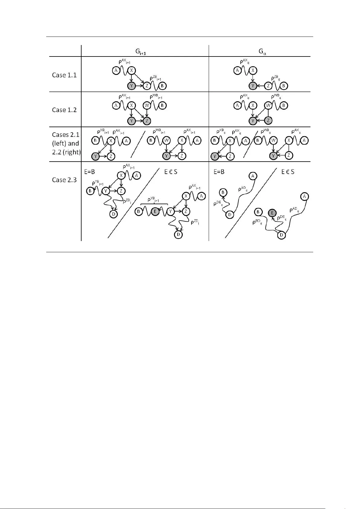
FINDING CONSENSUS BA YESIAN NETW ORK STR UCTURES JOSE M. PE ˜ NA ADIT, DEP AR TMENT OF COMPUTER AND INF ORMA TION SCIENCE LINK ¨ OPING UNIVERSITY, SE-58183 LINK ¨ OPING, SWEDEN JOSE.M.PENA@LIU.SE Abstract. Supp ose that m ultiple exp erts (or learning algorithms) provide us with alterna- tiv e Ba yesian net work (BN) structures o v er a domain, and that we are in terested in combining them in to a single consensus BN structure. Sp ecifically , we are in terested in that the con- sensus BN structure only represents indep endences all the given BN structures agree up on and that it has as few parameters asso ciated as p ossible. In this pap er, we prov e that there ma y exist several non-equiv alen t consensus BN structures and that finding one of them is NP-hard. Th us, w e decide to resort to heuristics to find an approximated consensus BN structure. In this pap er, we consider the heuristic prop osed in (Matzkevic h and Abramson, 1992, 1993a,b). This heuristic builds up on tw o algorithms, called Metho ds A and B, for effi- cien tly deriving the minimal directed indep endence map of a BN structure relativ e to a given no de ordering. Metho ds A and B are claimed to b e correct although no pro of is provided (a pro of is just sketc hed). In this pap er, w e show that Methods A and B are not correct and prop ose a correction of them. 1. Introduction Ba y esian netw orks (BNs) are a p opular graphical formalism for representing probabilit y distributions. A BN consists of structure and parameters. The structure, a directed and acyclic graph (DA G), induces a set of indep endencies that the represen ted probability distri- bution satisfies. The parameters sp ecify the conditional probabilit y distribution of eac h no de giv en its parents in the structure. The BN represents the probabilit y distribution that results from the pro duct of these conditional probability distributions. T ypically , a single exp ert (or learning algorithm) is consulted to construct a BN of the domain at hand. Therefore, there is a risk that the so-constructed BN is not as accurate as it could b e if, for instance, the exp ert has a bias or o verlooks certain details. One wa y to minimize this risk consists in obtaining m ultiple BNs of the domain from multiple exp erts and, then, combining them into a single consensus BN. This approac h has received significant attention in the literature (Matzkevic h and Abramson, 1992, 1993a,b; Maynard-Reid I I and Cha jewsk a, 2001; Nielsen and Parsons, 2007; P enno ck and W ellman, 1999; Ric hardson and Domingos, 2003; del Sagrado and Moral, 2003). The most relev ant of these references is probably (Pennock and W ellman, 1999), b e- cause it shows that ev en if the exp erts agree on the BN structure, no metho d for combining the exp erts’ BNs pro duces a consensus BN that resp ects some reasonable assumptions and whose structure is the agreed BN structure. Unfortunately , this problem is often o verlooked. T o a v oid it, w e propose to com bine the experts’ BNs in t w o steps. First, finding the consensus BN s tructure and, then, finding the consensus parameters for the consensus BN structure. This pap er fo cuses only on the first step. Sp ecifically , we assume that multiple exp erts pro- vide us with alternative DA G mo dels of a domain, and we are interested in combining them in to a single consensus D A G. Sp ecifically , we are interested in that the consensus DA G only represen ts indep endences all the given D A Gs agree up on and as many of them as p ossible. In other words, the consensus DA G is the D A G that represents the most indep endences among all the minimal directed indep endence (MDI) maps of the in tersection of the indep endence Date : Octob er 26, 2018. 1 2 mo dels induced by the given DA Gs. 1 T o our knowledge, whether the consensus DA G can or cannot b e found efficien tly is still an op en problem. See (Matzk evic h and Abramson, 1992, 1993a,b) for more information. In this pap er, w e redefine the consensus DA G as the DA G that has the fewest parameters asso ciated among all the MDI maps of the intersection of the indep endence mo dels induced by the given D A Gs. This definition is in line with that of finding a D A G to represen t a probabilit y distribution p . The desired D AG is t ypically defined as the MDI map of p that has the fewest parameters asso ciated rather than as the MDI map of p that represen ts the most indep endences. See, for instance, (Chick ering et al., 2004). The n um b er of parameters asso ciated with a DA G is a measure of the complexit y of the DA G, since it is the num ber of parameters required to sp ecify all the probabilit y distributions that can b e represented by the DA G. In this pap er, w e pro v e that there may exist several non-equiv alent consensus DA Gs and that finding one of them is NP-hard. Thus, w e decide to resort to heuristics to find an appro x- imated consensus D A G. In this pap er, we consider the following heuristic due to Matzkevic h and Abramson (1992, 1993a,b). First, let α denote any ordering of the no des in the given D A Gs, whic h w e denote here as G 1 , . . . , G m . Then, find the MDI map G i α of eac h G i rela- tiv e to α . Finally , let the approximated consensus D A G b e the DA G whose arcs are exactly the union of the arcs in G 1 α , . . . , G m α . It should b e men tioned that our formulation of the heuristic differs from that in (Matzkevic h and Abramson, 1992, 1993a,b) in the following tw o p oin ts. First, the heuristic was introduced under the original definition of consensus DA G. W e justify later that the heuristic also makes sense under our definition of consensus D A G. Second, α was originally required to b e consistent with one of the given DA Gs. W e remo v e this requiremen t. All in all, a k ey step in the heuristic is finding the MDI map G i α of eac h G i . Since this task is not trivial, Matzk evic h and Abramson (1993b) present t wo algorithms, called Metho ds A and B, for efficien tly deriving G i α from G i . Metho ds A and B are claimed to b e correct although no pro of is pro vided (a pro of is just sk etc hed). In this pap er, we show that Metho ds A and B are not correct and prop ose a correction of them. As said, we are not the first to study the problem of finding the consensus D A G. In addition to the w orks discussed ab o ve by Matzkevic h and Abramson (1992, 1993a,b) and Pennock and W ellman (1999), some other w orks devoted to this problem are (Ma ynard-Reid I I and Cha jewsk a, 2001; Nielsen and Parsons, 2007; Richardson and Domingos, 2003; del Sagrado and Moral, 2003). W e elab orate b elow on the differences b etw een these w orks and ours. Ma ynard-Reid I I and Cha jewsk a (2001) prop ose to adapt existing score-based algorithms for learning D A Gs from data to the case where the learning data is replaced by the BNs pro vided b y some exp erts. Their approac h suffers the problem p ointed out by Pennock and W ellman (1999), b ecause it consists essentially in learning a consensus D A G from a com bination of the giv en BNs. A somehow related approach is prop osed by Richardson and Domingos (2003). Sp ecifically , they prop ose a Bay esian approach to learning DA Gs from data, where the prior probabilit y distribution ov er DA Gs is constructed from the D A Gs provided by some exp erts. Since their approac h requires data and do es not com bine the given DA Gs into a single D A G, it addresses a problem rather differen t from the one in this pap er. Moreov er, the construction of the prior probability distribution ov er DA Gs ignores the fact that some giv en DA Gs may b e differen t but equiv alen t. That is, unlik e in the present work, a DA G is not in terpreted as inducing an indep endence mo del. A w ork that is relativ ely close to ours is that b y del Sagrado and Moral (2003). Sp ecifically , they sho w ho w to construct a MDI map of the in tersection and union of the indep endence mo dels induced by the D AGs pro vided b y some exp erts. Ho w ev er, 1 It is worth mentioning that the term consensus DA G has a different meaning in computational biology (Jac kson et al., 2005). There, the consensus DA G of a given set of DA Gs G 1 , . . . , G m is defined as the DA G that contains the most of the arcs in G 1 , . . . , G m . Therefore, the difficulty lies in keeping as many arcs as p ossible without creating cycles. Note that, unlike in the present w ork, a DA G is not interpreted as inducing an indep endence mo del in (Jac kson et al., 2005). 3 there are three main differences b etw een their w ork and ours. First, unlike us, they do not assume that the given DA Gs are defined ov er the same set of no des. Second, unlik e us, they assume that there exists a no de ordering that is consisten t with all the giv en DA Gs. Third, their goal is to find a MDI map whereas ours is to find the MDI map that has the fewest parameters asso ciated among all the MDI maps, i.e. the consensus DA G. Finally , Nielsen and P arsons (2007) dev elop a general framework to construct the consensus DA G gradually . Their framework is general in the sense that it is not tailored to any particular definition of consensus DA G. Instead, it relies up on a score to b e defined b y the user and that each exp ert will use to score different extensions to the curren t partial consensus DA G. The individual scores are then com bined to c ho ose the extension to p erform. Unfortunately , we do not see ho w this framework could b e applied to our definition of consensus DA G. Sp ecifically , w e do not see how eac h exp ert could score the extensions indep enden tly of the other exp erts, what the score w ould lo ok like, or how the scores w ould b e combined. It is w orth recalling that this pap er deals with the com bination of probability distributions expressed as BNs. Those readers in terested in the com bination of probabilit y distributions expressed in non-graphical numerical forms are referred to, for instance, (Genest and Zidek, 1986). Note also that w e are interested in the combination b efore an y data is observ ed. Those readers in terested in the com bination after some data has b een observ ed and eac h exp ert has up dated her b eliefs accordingly are referred to, for instance, (Ng and Abramson, 1994). Finally , note also that w e aim at com bining the giv en D A Gs in to a D A G, the consensus DA G. Those readers interested in finding not a DA G but graphical features (e.g. arcs or paths) all or a significan t num ber of exp erts agree up on may wan t to consult (F riedman and Koller, 2003; Hartemink et al., 2002; P e ˜ na et al., 2004), since these w orks deal with a similar problem. The rest of the pap er is organized as follows. W e start by reviewing some preliminary concepts in Section 2. W e analyze the complexity of finding the consensus D A G in Section 3. W e discuss the heuristic for finding an approximated consensus DA G in more detail in Section 4. W e introduce Metho ds A and B in Section 5 and show that they are not correct. W e correct them in Section 6. W e analyze the complexit y of the corrected Metho ds A and B in Section 7 and show that they are more efficien t than any other approach w e can think of to solv e the same problem. W e close with some discussion in Section 8. 2. Preliminaries In this section, we review some concepts used in this pap er. All the D A Gs, probabilit y distributions and indep endence mo dels in this pap er are defined o v er V , unless otherwise stated. If A → B is in a D A G G , then we sa y that A and B are adjac ent in G . Moreo v er, w e sa y that A is a p ar ent of B and B a child of A in G . W e denote the parents of B in G b y P a G ( B ). A no de is called a sink no de in G if it has no c hildren in G . A r oute b et w een t w o no des A and B in G is a sequence of no des starting with A and ending with B such that every t w o consecutive no des in the sequence are adjacent in G . Note that the no des in a route are not necessarily distinct. The length of a route is the num ber of (not necessarily distinct) arcs in the route. W e treat all the no des in G as routes of length zero. A route b et ween A and B is called desc ending from A to B if all the arcs in the route are directed to w ards B . If there is a descending route from A to B , then B is called a desc endant of A . Note that A is a descendant of itself, since we allo w routes of length zero. Giv en a subset X ⊆ V , a no de A ∈ X is called maximal in G if A is not descendan t of an y no de in X \ { A } in G . Giv en a route ρ b etw een A and B in G and a route ρ 0 b et ween B and C in G , ρ ∪ ρ 0 denotes the route b etw een A and C in G resulting from app ending ρ 0 to ρ . The numb er of p ar ameters asso ciated with a D A G G is P B ∈ V [ Q A ∈ P a G ( B ) r A ]( r B − 1), where r A and r B are the n umbers of states of the random v ariables corresp onding to the no de A and B . An arc A → B in G is said to b e c over e d if P a G ( A ) = P a G ( B ) \ { A } . By c overing an arc A → B in G w e mean adding to G the smallest set of arcs so that A → B b ecomes 4 co v ered. W e say that a no de C is a c ol lider in a route in a DA G if there exist tw o no des A and B such that A → C ← B is a subroute of the route. Note that A and B ma y coincide. Let X , Y and Z denote three disjoin t subsets of V . A route in a DA G is said to b e Z -active when (i) ev ery collider no de in the route is in Z , and (ii) every non-collider no de in the route is outside Z . When there is no route in a D A G G b etw een a no de in X and a no de in Y that is Z -active, we sa y that X is sep ar ate d from Y giv en Z in G and denote it as X ⊥ G Y | Z . W e denote b y X 6⊥ G Y | Z that X ⊥ G Y | Z do es not hold. This definition of separation is equiv alen t to other more common definitions (Studen ´ y, 1998, Section 5.1). Let X , Y , Z and W denote four disjoin t subsets of V . Let us abbreviate X ∪ Y as XY . An indep endenc e mo del M is a set of statemen ts of the form X ⊥ M Y | Z , meaning that X is indep enden t of Y giv en Z . Given a subset U ⊆ V , w e denote b y [ M ] U all the statemen ts in M suc h that X , Y , Z ⊆ U . Given t w o indep endence mo dels M and N , w e denote by M ⊆ N that if X ⊥ M Y | Z then X ⊥ N Y | Z . W e sa y that M is a gr aphoid if it satisfies the follo wing prop erties: symmetry X ⊥ M Y | Z ⇒ Y ⊥ M X | Z , de c omp osition X ⊥ M YW | Z ⇒ X ⊥ M Y | Z , we ak union X ⊥ M YW | Z ⇒ X ⊥ M Y | ZW , c ontr action X ⊥ M Y | ZW ∧ X ⊥ M W | Z ⇒ X ⊥ M YW | Z , and interse ction X ⊥ M Y | ZW ∧ X ⊥ M W | ZY ⇒ X ⊥ M YW | Z . The indep endence mo del induc e d by a pr ob ability distribution p , denoted as I ( p ), is the set of probabilistic indep endences in p . The indep endence mo del induc e d by a D AG G , denoted as I ( G ), is the set of separation statements X ⊥ G Y | Z . It is kno wn that I ( G ) is a graphoid (Studen ´ y and Bouc k aert, 1998, Lemma 3.1). Moreov er, I ( G ) satisfies the c omp osition prop erty X ⊥ G Y | Z ∧ X ⊥ G W | Z ⇒ X ⊥ G YW | Z (Chic k ering and Meek, 2002, Prop osition 1). Two DA Gs G and H are called e quivalent if I ( G ) = I ( H ). A DA G G is a dir e cte d indep endenc e map of an indep endence mo del M if I ( G ) ⊆ M . Moreo v er, G is a minimal directed indep endence (MDI) map of M if removing any arc from G makes it cease to b e a directed indep endence map of M . W e say that G and an ordering of its no des are c onsistent when, for every arc A → B in G , A precedes B in the no de ordering. W e sa y that a D A G G α is a MDI map of an indep endence mo del M r elative to a no de or dering α if G α is a MDI map of M and G α is consistent with α . If M is a graphoid, then G α is unique (P earl, 1988, Theorems 4 and 9). Sp ecifically , for eac h no de A , P a G α ( A ) is the smallest subset X of the predecessors of A in α , P r e α ( A ), suc h that A ⊥ M P r e α ( A ) \ X | X . 3. Finding a Consensus D A G is NP-Hard Recall that we hav e defined the consensus D AG of a giv en set of DA Gs G 1 , . . . , G m as the D A G that has the few est parameters asso ciated among all the MDI maps of ∩ m i =1 I ( G i ). A sensible wa y to start the quest for the consensus D A G is b y inv estigating whether there can exist sev eral non-equiv alen t consensus DA Gs. The follo wing theorem answers this question. Theorem 1. Ther e exists a set of D AGs that has two non-e quivalent c onsensus DA Gs. Pr o of. Consider the follo wing tw o DA Gs o v er four random v ariables with the same num b er of states eac h: I ← J ↓ K → L I → J ↓ K ← L An y of the follo wing tw o non-equiv alen t D A Gs is the consensus DA G of the tw o D AGs ab o ve: I → J ↓ & ↑ K ← L I ← J ↑ % ↓ K → L  5 A natural follo w-up question to inv estigate is whether a consensus DA G can b e found effi- cien tly . Unfortunately , finding a consensus DA G is NP-hard, as w e prov e b elow. Sp ecifically , w e pro ve that the following decision problem is NP-hard: CONSENSUS • INST ANCE: A set of DA Gs G 1 , . . . , G m o v er V , and a p ositive integer d . • QUESTION: Do es there exist a DA G G o ver V suc h that I ( G ) ⊆ ∩ m i =1 I ( G i ) and the n um b er of parameters asso ciated with G is not greater than d ? Pro ving that CONSENSUS is NP-hard implies that finding the consensus D A G is also NP-hard, b ecause if there existed an efficient algorithm for finding the consensus DA G, then w e could use it to solv e CONSENSUS efficiently . Our pro of makes use of the following tw o decision problems: FEEDBA CK AR C SET • INST ANCE: A directed graph G = ( V , A ) and a p ositive integer k . • QUESTION: Do es there exist a subset B ⊂ A such that | B | ≤ k and B has at least one arc from every directed cycle in G ? LEARN • INST ANCE: A probability distribution p ov er V , and a p ositive integer d . • QUESTION: Does there exist a D A G G ov er V such that I ( G ) ⊆ I ( p ) and the num ber of parameters asso ciated with G is not greater than d ? FEEDBA CK ARC SET is NP-complete (Garey and Johnson, 1979). FEEDBA CK ARC SET remains NP-complete for directed graphs in whic h the total degree of each vertex is at most three (Ga vril, 1977). This degree-b ounded FEEDBACK ARC SET problem is used in (Chic k ering et al., 2004) to prov e that LEARN is NP-hard. In their pro of, Chick ering et al. (2004) use the follo wing p olynomial reduction of any instance of the degree-b ounded FEEDBA CK AR C SET into an instance of LEARN: • Let the instance of the degree-b ounded FEEDBA CK ARC SET consist of the directed graph F = ( V F , A F ) and the p ositive integer k . • Let L denote a D A G whose no des and arcs are determined from F as follows. F or ev ery arc V F i → V F j in A F , create the following no des and arcs in L : A ij (9) D ij (9) ↓ ↓ V F i (9) → B ij (2) H ij (2) E ij (2) ← G ij (9) ↓ . & ↓ C ij (3) F ij (2) → V F j (9) The num ber in paren thesis b esides eac h no de is the n um b er of states of the corre- sp onding random v ariable. Let H L denote all the no des H ij in L , and let V L denote the rest of the no des in L . • Sp ecify a (join) probabilit y distribution p ( H L , V L ) suc h that I ( p ( H L , V L )) = I ( L ). • Let the instance of LEARN consist of the (marginal) probability distribution p ( V L ) and the p ositive in teger d , where d is computed from F and k as shown in (Chic k ering et al., 2004, Equation 2). W e now describ e ho w the instance of LEARN resulting from the reduction ab ov e can b e further reduced in to an instance of CONSENSUS in p olynomial time: • Let C 1 denote the D A G ov er V L that has all and only the arcs in L whose b oth endp oin ts are in V L . • Let C 2 denote the D A G ov er V L that only has the arcs B ij → C ij ← F ij for all i and j . 6 • Let C 3 denote the D A G ov er V L that only has the arcs C ij → F ij ← E ij for all i and j . • Let the instance of CONSENSUS consist of the DA Gs C 1 , C 2 and C 3 , and the p ositiv e in teger d . Theorem 2. CONSENSUS is NP-har d. Pr o of. W e start by pro ving that there is a p olynomial reduction of an y instance F of the degree-b ounded FEEDBACK AR C SET in to an instance C of CONSENSUS. First, reduce F into an instance L of LEARN as shown in (Chick ering et al., 2004) and, then, reduce L in to C as shown ab o v e. W e now prov e that there is a solution to F iff there is a solution to C . Theorems 8 and 9 in (Chick ering et al., 2004) prov e that there is a solution to F iff there is a solution to L . Therefore, it only remains to prov e that there is a solution to L iff there is a solution to C . Let L and p ( H L , V L ) denote the D A G and the probability distribution constructed in the reduction of F in to L . Recall that I ( p ( H L , V L )) = I ( L ). Moreo v er: • Let L 1 denote the DA G ov er ( H L , V L ) that has all and only the arcs in L whose b oth endp oin ts are in V L . • Let L 2 denote the D AG ov er ( H L , V L ) that only has the arcs B ij → C ij ← H ij → F ij for all i and j . • Let L 3 denote the DA G ov er ( H L , V L ) that only has the arcs C ij ← H ij → F ij ← E ij for all i and j . Note that any separation statement that holds in L also holds in L 1 , L 2 and L 3 . Then, I ( p ( H L , V L )) = I ( L ) ⊆ ∩ 3 i =1 I ( L i ) and, thus, I ( p ( V L )) ⊆ [ ∩ 3 i =1 I ( L i )] V L = ∩ 3 i =1 [ I ( L i )] V L . Let C 1 , C 2 and C 3 denote the DA Gs constructed in the reduction of L into C . Note that [ I ( L i )] V L = I ( C i ) for all i . Then, I ( p ( V L )) ⊆ ∩ 3 i =1 I ( C i ) and, thus, if there is a solution to L then there is a solution to C . W e no w pro v e the opp osite. The pro of is essen tially the same as that of (Chick ering et al., 2004, Theorem 9). Let us define the ( V i , V j ) edge comp onen t of a D A G G o v er V L as the subgraph of G that has all and only the arcs in G whose b oth endp oin ts are in { V i , A ij , B ij , C ij , D ij , E ij , F ij , G ij , V j } . Giv en a solution C to C , w e create another solution C 0 to C as follows: • Initialize C 0 to C 1 . • F or every ( V i , V j ) edge comp onen t of C , if there is no directed path in C from V i to V j , then add to C 0 the arcs E ij → C ij ← F ij . • F or every ( V i , V j ) edge comp onent of C , if there is a directed path in C from V i to V j , then add to C 0 the arcs B ij → F ij ← C ij . Note that C 0 is acyclic b ecause C is acyclic. Moreo v er, I ( C 0 ) ⊆ ∩ 3 i =1 I ( C i ) b ecause I ( C 0 ) ⊆ I ( C i ) for all i . In order to b e able to conclude that C 0 is a solution to C , it only remains to pro v e that the n um b er of parameters asso ciated with C 0 is not greater than d . Specifically , w e pro ve b elow that C 0 do es not hav e more parameters asso ciated than C , which has less than d parameters asso ciated b ecause it is a solution to C . As seen b efore, I ( C 0 ) ⊆ I ( C 1 ). Likewise, I ( C ) ⊆ I ( C 1 ) b ecause C is a solution to C . Th us, there exists a sequence S (resp. S 0 ) of cov ered arc reversals and arc additions that transforms C 1 in to C (resp. C 0 ) (Chick ering, 2002, Theorem 4). Note that a cov ered arc rev ersal do es not mo dify the n umber of parameters asso ciated with a DA G, whereas an arc addition increases it (Chic k ering, 1995, Theorem 3). Th us, S and S 0 monotonically increase the num ber of parameters asso ciated with C 1 as they transform it. Recall that C 1 consists of a series of edge comp onents of the form 7 A ij (9) D ij (9) ↓ ↓ V F i (9) → B ij (2) E ij (2) ← G ij (9) ↓ ↓ C ij (3) F ij (2) → V F j (9) The num ber in paren thesis b esides each no de is the num ber of states of the corresp onding random v ariable. Let us study how the sequences S and S 0 mo dify eac h edge comp onen t of C 1 . S 0 simply adds the arcs B ij → F ij ← C ij or the arcs E ij → C ij ← F ij . Note that adding the first pair of arcs results in an increase of 10 parameters, whereas adding the second pair of arcs results in an increase of 12 parameters. Unlike S 0 , S ma y reverse some arc in the edge comp onen t. If that is the case, then S m ust cov er the arc first, whic h implies an increase of at least 16 parameters (co v ering F ij → V j b y adding E ij → V j implies an increase of exactly 16 parameters, whereas any other arc co v ering implies a larger increase). Then, S implies a larger increase in the num ber of parameters than S 0 . On the other hand, if S do es not rev erse an y arc in the edge comp onen t, then S simply adds the arcs that are in C but not in C 1 . Note that either C ij → F ij or C ij ← F ij is in C , b ecause otherwise C ij ⊥ C F ij | Z for some Z ⊂ V L whic h con tradicts the fact that C is a solution to C since C ij 6⊥ C 2 F ij | Z . If C ij → F ij is in C , then either B ij → F ij or B ij ← F ij is in C b ecause otherwise B ij ⊥ C F ij | Z for some Z ⊂ V L suc h that C ij ∈ Z , which con tradicts the fact that C is a solution to C since B ij 6⊥ C 2 F ij | Z . As B ij ← F ij w ould create a cycle in C , B ij → F ij is in C . Therefore, S adds the arcs B ij → F ij ← C ij and, by construction of C 0 , S 0 also adds them. Th us, S implies an increase of at least as man y parameters as S 0 . On the other hand, if C ij ← F ij is in C , then either C ij → E ij or C ij ← E ij is in C because otherwise C ij ⊥ C E ij | Z for some Z ⊂ V L suc h that F ij ∈ Z , whic h con tradicts the fact that C is a solution to C since C ij 6⊥ C 3 E ij | Z . As C ij → E ij w ould create a cycle in C , C ij ← E ij is in C . Therefore, S adds the arcs E ij → C ij ← F ij and, b y construction of C 0 , S 0 adds either the arcs E ij → C ij ← F ij or the arcs B ij → F ij ← C ij . In any case, S implies an increase of at least as many parameters as S 0 . Consequently , C 0 do es not hav e more parameters asso ciated than C . Finally , note that I ( p ( V L )) ⊆ I ( C 0 ) b y (Chic k ering et al., 2004, Lemma 7). Thus, if there is a solution to C then there is a solution to L .  It is worth noting that our pro of ab o ve con tains t wo restrictions. First, the n um b er of D A Gs to consensuate is three. Second, the num ber of states of each random v ariable in V L is not arbitrary but prescrib ed. The first restriction is easy to relax: Our pro of can b e extended to consensuate more than three DA Gs by simply letting C i b e a DA G ov er V L with no arcs for all i > 3. Ho wev er, it is an op en question whether CONSENSUS remains NP-hard when the num b er of DA Gs to consensuate is t wo and/or the num ber of states of each random v ariable in V L is arbitrary . The follo wing theorem strentghens the previous one. Theorem 3. CONSENSUS is NP-c omplete. Pr o of. By Theorem 2, all that remains to prov e is that CONSENSUS is in NP , i.e. that we can v erify in p olynomial time if a given D A G G is a solution to a given instance of CONSENSUS. Let α denote any no de ordering that is consisten t with G . The causal list of G relativ e to α is the set of separation statements A ⊥ G P r e α ( A ) \ P a G ( A ) | P a G ( A ) for all no de A . It is kno wn that I ( G ) coincides with the closure with resp ect to the graphoid prop erties of the causal list of G relative to α (P earl, 1988, Corollary 7). Therefore, I ( G ) ⊆ ∩ m i =1 I ( G i ) iff A ⊥ G i P r e α ( A ) \ P a G ( A ) | P a G ( A ) for all 1 ≤ i ≤ m , b ecause ∩ m i =1 I ( G i ) is a graphoid (del Sagrado and Moral, 2003, Corollary 1). Let n , a and a i denote, resp ectively , the num ber of no des in G , the n umber of arcs in G , and the n um b er of arcs in G i . Let b = max 1 ≤ i ≤ m a i . 8 Chec king a separation statemen t in G i tak es O ( a i ) time (Geiger et al., 1990, p. 530). Then, c hec king whether I ( G ) ⊆ ∩ m i =1 I ( G i ) tak es O ( mnb ) time. Finally , note that computing the n um b er of parameters asso ciated with G tak es O ( a ).  4. Finding an Appro xima ted Consensus DA G Since finding a consensus DA G of some giv en DA Gs is NP-hard, we decide to resort to heuristics to find an approximated consensus D A G. This do es not mean that we discard the existence of fast sup er-p olynomial algorithms. It simply means that w e do not pursue that p ossibilit y in this pap er. Sp ecifically , in this pap er w e consider the following heuristic due to Matzk evic h and Abramson (1992, 1993a,b). First, let α denote an y ordering of the no des in the given D AGs, whic h w e denote here as G 1 , . . . , G m . Then, find the MDI map G i α of each G i relativ e to α . Finally , let the approximated consensus D A G b e the DA G whose arcs are exactly the union of the arcs in G 1 α , . . . , G m α . The following theorem justifies taking the union of the arcs. Sp ecifically , it pro v es that the DA G returned by the heuristic is the consensus D A G if this was required to b e consisten t with α . Theorem 4. The D A G H r eturne d by the heuristic ab ove is the D A G that has the fewest p ar ameters asso ciate d among al l the MDI maps of ∩ m i =1 I ( G i ) r elative to α . Pr o of. W e start by proving that H is a MDI map of ∩ m i =1 I ( G i ). First, w e show that I ( H ) ⊆ ∩ m i =1 I ( G i ). It suffices to note that I ( H ) ⊆ ∩ m i =1 I ( G i α ) b ecause each G i α is a subgraph of H , and that ∩ m i =1 I ( G i α ) ⊆ ∩ m i =1 I ( G i ) b ecause I ( G i α ) ⊆ I ( G i ) for all i . No w, assume to the con trary that the DA G H 0 resulting from removing an arc A → B from H satis- fies that I ( H 0 ) ⊆ ∩ m i =1 I ( G i ). By construction of H , A → B is in G i α for some i , sa y i = j . Note that B ⊥ H 0 P r e α ( B ) \ P a H 0 ( B ) | P a H 0 ( B ), which implies B ⊥ G j P r e α ( B ) \ (( ∪ m i =1 P a G i α ( B )) \ { A } ) | ( ∪ m i =1 P a G i α ( B )) \ { A } b ecause P a H 0 ( B ) = ( ∪ m i =1 P a G i α ( B )) \ { A } and I ( H 0 ) ⊆ ∩ m i =1 I ( G i ). Note also that B ⊥ G j α P r e α ( B ) \ P a G j α ( B ) | P a G j α ( B ), whic h implies B ⊥ G j P r e α ( B ) \ P a G j α ( B ) | P a G j α ( B ) b ecause I ( G j α ) ⊆ I ( G j ). Therefore, B ⊥ G j P r e α ( B ) \ ( P a G j α ( B ) \ { A } ) | P a G j α ( B ) \ { A } by in tersection. How ev er, this con tradicts the fact that G j α is the MDI map of G j relativ e to α . Then, H is a MDI map of ∩ m i =1 I ( G i ) relativ e to α . Finally , note that ∩ m i =1 I ( G i ) is a graphoid (del Sagrado and Moral, 2003, Corollary 1). Consequen tly , H is the only MDI map of ∩ m i =1 I ( G i ) relativ e to α .  A k ey step in the heuristic ab ov e is, of course, c ho osing a go o d no de ordering α . Unfortu- nately , the fact that CONSENSUS is NP-hard implies that it is also NP-hard to find the b est no de ordering α , i.e. the no de ordering that mak es the heuristic to return the MDI map of ∩ m i =1 I ( G i ) that has the few est parameters asso ciated. T o see it, note that if there existed an efficien t algorithm for finding the b est no de ordering, then Theorem 4 w ould imply that we could solv e CONSENSUS efficiently by running the heuristic with the b est no de ordering. In the last sen tence, w e ha v e implicitly assumed that the heuristic is efficien t, whic h implies that w e hav e implicitly assumed that w e can efficiently find the MDI map G i α of eac h G i . The rest of this pap er shows that this assumption is correct. 5. Methods A and B are not Correct Matzk evic h and Abramson (1993b) do not only propose the heuristic discussed in the previous section, but they also presen t tw o algorithms, called Metho ds A and B, for efficiently deriving the MDI map G α of a D A G G relativ e to a no de ordering α . The algorithms work iterativ ely b y cov ering and reversing an arc in G until the resulting DA G is consistent with α . It is ob vious that suc h a w a y of w orking produces a directed indep endence map of G . Ho w ev er, in order to arrive at G α , the arc to cov er and reverse in eac h iteration m ust b e 9 Construct β ( G , α ) /* Given a DA G G and a no de ordering α , the algorithm returns a no de ordering β that is consistent with G and as close to α as p ossible */ 1 β = ∅ 2 G 0 = G 3 Let A denote a sink no de in G 0 /* 3 Let A denote the rightmost no de in α that is a sink no de in G 0 */ 4 Add A as the leftmost no de in β 5 Let B denote the right neighbor of A in β 6 If B 6 = ∅ and A / ∈ P a G ( B ) and A is to the righ t of B in α then 7 In terchange A and B in β 8 Go to line 5 9 Remov e A and all its incoming arcs from G 0 10 If G 0 6 = ∅ then go to line 3 11 Return β Metho d A( G , α ) /* Given a DA G G and a no de ordering α , the algorithm returns G α */ 1 β =Construct β ( G , α ) 2 Let Y denote the leftmost no de in β whose left neighbor in β is to its right in α 3 Let Z denote the left neighbor of Y in β 4 If Z is to the right of Y in α then 5 If Z → Y is in G then cov er and reverse Z → Y in G 6 In terchange Y and Z in β 7 Go to line 3 8 If β 6 = α then go to line 2 9 Return G Metho d B( G , α ) /* Given a DA G G and a no de ordering α , the algorithm returns G α */ 1 β =Construct β ( G , α ) 2 Let Y denote the leftmost no de in β whose right neighbor in β is to its left in α 3 Let Z denote the right neighbor of Y in β 4 If Z is to the left of Y in α then 5 If Y → Z is in G then co ver and reverse Y → Z in G 6 In terchange Y and Z in β 7 Go to line 3 8 If β 6 = α then go to line 2 9 Return G Figure 1. Construct β , and Metho ds A and B. Our correction of Construct β consists in replacing line 3 with the line in comment s under it. carefully chosen. The pseudo co de of Metho ds A and B can b e seen in Figure 1. Metho d A starts by calling Construct β to derive a no de ordering β that is consistent with G and as 10 Figure 2. A counterexample to the correctness of Metho ds A and B. close to α as p ossible (line 6). By β b eing as close to α as p ossible, we mean that the num ber of arcs Metho ds A and B will later cov er and reverse is kept at a minim um, b ecause Metho ds A and B will use β to c ho ose the arc to co v er and rev erse in eac h iteration. In particular, Metho d A finds the leftmost no de in β that should be in terc hanged with its left neigh b or (line 2) and it rep eatedly in terc hanges this no de with its left neigh b or (lines 3-4 and 6-7). Eac h of these interc hanges is preceded by cov ering and reversing the corresp onding arc in G (line 5). Metho d B is essentially identical to Metho d A. The only differences b etw een them are that the word ”right” is replaced by the word ”left” and vice versa in lines 2-4, and that the arcs p oint in opp osite directions in line 5. Metho ds A and B are claimed to b e correct in (Matzk evich and Abramson, 1993b, Theorem 4 and Corollary 2) although no pro of is pro vided (a pro of is just sk etc hed). The follo wing coun terexample sho ws that Metho ds A and B are actually not correct. Let G b e the D A G in the left-hand side of Figure 2. Let α = ( M , I , K, J, L ). Then, w e can make use of the c haracterization introduced in Section 2 to see that G α is the DA G in the center of Figure 2. Ho w ev er, Metho ds A and B return the DA G in the right-hand side of Figure 2. T o see it, w e follo w the execution of Metho ds A and B step b y step. First, Metho ds A and B construct β b y calling Construct β , which runs as follo ws: (1) Initially , β = ∅ and G 0 = G . (2) Select the sink no de M in G 0 . Then, β = ( M ). Remov e M and its incoming arcs from G 0 . (3) Select the sink node L in G 0 . Then, β = ( L, M ). No interc hange in β is p erformed b ecause L ∈ P a G ( M ). Remov e L and its incoming arcs from G 0 . (4) Select the sink no de K in G 0 . Then, β = ( K , L, M ). No interc hange in β is p erformed b ecause K is to the left of L in α . Remov e K and its incoming arcs from G 0 . (5) Select the sink no de J in G 0 . Then, β = ( J, K , L, M ). No interc hange in β is p erformed b ecause J ∈ P a G ( K ). (6) Select the sink no de I in G 0 . Then, β = ( I , J , K, L, M ). No interc hange in β is p erformed b ecause I is to the left of J in α . When Construct β ends, Metho ds A and B contin ue as follo ws: (7) Initially , β = ( I , J, K , L, M ). 11 (8) Add the arc I → J and reverse the arc J → K in G . Interc hange J and K in β . Then, β = ( I , K , J , L, M ). (9) Add the arc J → M and reverse the arc L → M in G . Interc hange L and M in β . Then, β = ( I , K , J , M , L ). (10) Add the arcs I → M and K → M , and reverse the arc J → M in G . Interc hange J and M in β . Then, β = ( I , K, M , J , L ). (11) Reverse the arc K → M in G . Interc hange K and M in β . Then, β = ( I , M , K , J , L ). (12) Reverse the arc I → M in G . Interc hange I and M in β . Then, β = ( M , I , K , J, L ) = α . As a matter of fact, one can see as early as in step (8) ab ov e that Metho ds A and B will fail: One can see that I and M are not separated in the D AG resulting from step (8), which implies that I and M will not b e separated in the DA G returned b y Metho ds A and B, b ecause cov ering and reversing arcs nev er introduces new separation statements. Ho w ev er, I and M are separated in G α . Note that w e constructed β b y selecting first M , then L , then K , then J , and finally I . Ho w ev er, we could hav e selected first K , then I , then M , then L , and finally J , whic h would ha v e resulted in β = ( J, L, M , I , K ). With this β , Metho ds A and B return G α . Therefore, it mak es a difference whic h sink no de is selected in line 3 of Construct β . How ev er, Construct β ov erlooks this detail. W e prop ose correcting Construct β by replacing line 3 by ”Let A denote the righ tmost no de in α that is a sink no de in G 0 ”. Hereinafter, w e assume that an y call to Construct β is a call to the corrected v ersion thereof. The rest of this pap er is dev oted to pro v e that Metho ds A and B no w do return G α . 6. The Corrected Methods A and B are Correct Before proving that Metho ds A and B are correct, w e in tro duce some auxiliary lemmas. Their pro of can b e found in the app endix. Let us call p er c olating Y right-to-left in β to iterating through lines 3-7 in Metho d A while p ossible. Let us mo dify Metho d A by replacing line 2 b y ”Let Y denote the leftmost no de in β that has not b een considered b efore” and b y adding the chec k Z 6 = ∅ to line 4. The pseudo co de of the resulting algorithm, whic h w e call Metho d A2, can b e seen in Figure 3. Metho d A2 p ercolates right-to-left in β one b y one all the no des in the order in which they app ear in β . Lemma 1. Metho d A( G , α ) and Metho d A2( G , α ) r eturn the same D AG. Lemma 2. Metho d A2( G , α ) and Metho d B( G , α ) r eturn the same D AG. Let us call p er c olating Y left-to-right in β to iterating through lines 3-7 in Metho d B while p ossible. Let us mo dify Metho d B b y replacing line 2 by ”Let Y denote the rightmost no de in α that has not b een considered b efore” and b y adding the c hec k Z 6 = ∅ to line 4. The pseudo co de of the resulting algorithm, which w e call Metho d B2, can b e seen in Figure 3. Metho d B2 p ercolates left-to-righ t in β one by one all the no des in the reverse order in which they app ear in α . Lemma 3. Metho d B( G , α ) and Metho d B2( G , α ) r eturn the same D AG. W e are now ready to prov e the main result of this pap er. Theorem 5. L et G α denote the MDI map of a DA G G r elative to a no de or dering α . Then, Metho d A( G , α ) and Metho d B( G , α ) r eturn G α . Pr o of. By Lemmas 1-3, it suffices to prov e that Metho d B2( G , α ) returns G α . It is evident that Metho d B2 transforms β into α and, thus, that it halts at some p oint. Therefore, Metho d B2 p erforms a finite sequence of n modifications (arc additions and cov ered arc rev ersals) to G . Let G i denote the D A G resulting from the first i mo difications to G , and let G 0 = G . Sp ecifically , Metho d B2 constructs G i +1 from G i b y either (i) reversing the 12 Metho d A2( G , α ) /* Given a DA G G and a no de ordering α , the algorithm returns G α */ 1 β =Construct β ( G , α ) 2 Let Y denote the leftmost no de in β that has not b een considered b efore 3 Let Z denote the left neighbor of Y in β 4 If Z 6 = ∅ and Z is to the right of Y in α then 5 If Z → Y is in G then cov er and reverse Z → Y in G 6 In terchange Y and Z in β 7 Go to line 3 8 If β 6 = α then go to line 2 9 Return G Metho d B2( G , α ) /* Given a DA G G and a no de ordering α , the algorithm returns G α */ 1 β =Construct β ( G , α ) 2 Let Y denote the rightmost no de in α that has not b een considered b efore 3 Let Z denote the right neighbor of Y in β 4 If Z 6 = ∅ and Z is to the left of Y in α then 5 If Y → Z is in G then co ver and reverse Y → Z in G 6 In terchange Y and Z in β 7 Go to line 3 8 If β 6 = α then go to line 2 9 Return G Figure 3. Metho ds A2 and B2. co v ered arc Y → Z , or (ii) adding the arc X → Z for some X ∈ P a G i ( Y ) \ P a G i ( Z ), or (iii) adding the arc X → Y for some X ∈ P a G i ( Z ) \ P a G i ( Y ). Note that I ( G i +1 ) ⊆ I ( G i ) for all 0 ≤ i < n and, thus, that I ( G n ) ⊆ I ( G 0 ). W e start b y pro ving that G i is a DA G that is consisten t with β for all 0 ≤ i ≤ n . Since this is true for G 0 due to line 1, it suffices to prov e that if G i is a D A G that is consistent with β then so is G i +1 for all 0 ≤ i < n . W e consider the following four cases. Case 1: Method B2 constructs G i +1 from G i b y rev ersing the co v ered arc Y → Z . Then, G i +1 is a DA G b ecause rev ersing a cov ered arc do es not create an y cycle (Chick ering, 1995, Lemma 1). Moreo v er, note that Y and Z are interc hanged in β immediately after the co vered arc reversal. Thus, G i +1 is consisten t with β . Case 2: Method B2 constructs G i +1 from G i b y adding the arc X → Z for some X ∈ P a G i ( Y ) \ P a G i ( Z ). Note that X is to the left of Y and Y to the left of Z in β , b ecause G i is consisten t with β . Then, X is to the left of Z in β and, th us, G i +1 is a D A G that is consistent with β . Case 3: Method B2 constructs G i +1 from G i b y adding the arc X → Y for some X ∈ P a G i ( Z ) \ P a G i ( Y ). Note that X is to the left of Z in β b ecause G i is consistent with β , and Y is the left neighbor of Z in β (recall line 3). Then, X is to the left of Y in β and, th us, G i +1 is a D AG that is consistent with β . Case 4: Note that β ma y get mo dified b efore Metho d B2 constructs G i +1 from G i . Sp ecifically , this happ ens when Metho d B2 executes lines 5-6 but there is no arc 13 Figure 4. Different cases in the pro of of Theorem 5. Only the relev an t sub- graphs of G i +1 and G α are depicted. An undirected edge b etw een t w o no des denotes that the no des are adjacent. A curved edge betw een t w o no des denotes an S -activ e route b etw een the t w o no des. If the curved edge is directed, then the route is descending. A grey no de denotes a no de that is in S . b et ween Y and Z in G i . Ho wev er, the fact that G i is consistent with β b efore Y and Z are in terc hanged in β and the fact that Y and Z are neighbors in β (recall line 3) imply that G i is consisten t with β after Y and Z hav e b een in terc hanged. Since Metho d B2 transforms β into α , it follows from the result prov en ab ov e that G n is a D A G that is consistent with α . In order to prov e the theorem, i.e. that G n = G α , all that remains to prov e is that I ( G α ) ⊆ I ( G n ). T o see it, note that G n = G α follo ws from I ( G α ) ⊆ I ( G n ), I ( G n ) ⊆ I ( G 0 ), the fact that G n is a DA G that is consistent with α , and the fact that G α is the unique MDI map of G 0 relativ e to α . Recall that G α is guaran teed to b e unique b ecause I ( G 0 ) is a graphoid. The rest of the pro of is devoted to prov e that I ( G α ) ⊆ I ( G n ). Sp ecifically , we prov e that if I ( G α ) ⊆ I ( G i ) then I ( G α ) ⊆ I ( G i +1 ) for all 0 ≤ i < n . Note that this implies that I ( G α ) ⊆ I ( G n ) b ecause I ( G α ) ⊆ I ( G 0 ) by definition of MDI map. First, w e prov e it when Metho d B2 constructs G i +1 from G i b y reversing the co v ered arc Y → Z . That the arc reversed is co v ered implies that I ( G i +1 ) = I ( G i ) (Chick ering, 1995, Lemma 1). Th us, I ( G α ) ⊆ I ( G i +1 ) b ecause I ( G α ) ⊆ I ( G i ). No w, w e prov e that if I ( G α ) ⊆ I ( G i ) then I ( G α ) ⊆ I ( G i +1 ) for all 0 ≤ i < n when Metho d B2 constructs G i +1 from G i b y adding an arc. Sp ecifically , we prov e that if there is an S -active route ρ AB i +1 b et ween t wo no des A and B in G i +1 , then there is an S -active route b et w een A 14 and B in G α . W e prov e this result by induction on the n um b er of o ccurrences of the added arc in ρ AB i +1 . W e assume without loss of generalit y that the added arc o ccurs in ρ AB i +1 as few or few er times than in an y other S -active route b et w een A and B in G i +1 . W e call this the minimalit y prop erty of ρ AB i +1 . 2 If the n um b er of o ccurrences of the added arc in ρ AB i +1 is zero, then ρ AB i +1 is an S -activ e route betw een A and B in G i to o and, thus, there is an S -activ e route betw een A and B in G α since I ( G α ) ⊆ I ( G i ). Assume as induction h yp othesis that the result holds for up to k o ccurrences of the added arc in ρ AB i +1 . W e no w prov e it for k + 1 o ccurrences. W e consider the follo wing tw o cases. Eac h case is illustrated in Figure 4. Case 1: Method B2 constructs G i +1 from G i b y adding the arc X → Z for some X ∈ P a G i ( Y ) \ P a G i ( Z ). Note that X → Z o ccurs in ρ AB i +1 . 3 Let ρ AB i +1 = ρ AX i +1 ∪ X → Z ∪ ρ Z B i +1 . Note that X / ∈ S and ρ AX i +1 is S -active in G i +1 b ecause, otherwise, ρ AB i +1 w ould not b e S -activ e in G i +1 . Then, there is an S -active route ρ AX α b et ween A and X in G α b y the induction hypothesis. Moreov er, Y ∈ S b ecause, otherwise, ρ AX i +1 ∪ X → Y → Z ∪ ρ Z B i +1 w ould b e an S -activ e route betw een A and B in G i +1 that w ould violate the minimalit y prop ert y of ρ AB i +1 . Note that Y ← Z is in G α b ecause (i) Y and Z are adjacen t in G α since I ( G α ) ⊆ I ( G i ), and (ii) Z is to the left of Y in α (recall line 4). Note also that X → Y is in G α . T o see it, note that X and Y are adjacen t in G α since I ( G α ) ⊆ I ( G i ). Recall that Metho d B2 p ercolates left-to-righ t in β one by one all the no des in the rev erse order in which they app ear in α . Metho d B2 is currently p ercolating Y and, th us, the no des to the right of Y in α are to right of Y in β to o. If X ← Y were in G α then X would b e to the right of Y in α and, thus, X w ould b e to the right of Y in β . Ho w ev er, this would contradict the fact that X is to the left of Y in β , which follo ws from the fact that G i is consistent with β . Th us, X → Y is in G α . W e now consider t w o cases. Case 1.1: Assume that Z / ∈ S . Then, ρ Z B i +1 is S -active in G i +1 b ecause, otherwise, ρ AB i +1 w ould not b e S -active in G i +1 . Then, there is an S -active route ρ Z B α b et ween Z and B in G α b y the induction h yp othesis. Then, ρ AX α ∪ X → Y ← Z ∪ ρ Z B α is an S -activ e route b etw een A and B in G α . Case 1.2: Assume that Z ∈ S . Then, ρ Z B i +1 = Z ← W ∪ ρ W B i +1 . 4 Note that W / ∈ S and ρ W B i +1 is S -activ e in G i +1 b ecause, otherwise, ρ AB i +1 w ould not b e S -active in G i +1 . Then, there is an S -active route ρ W B α b et ween W and B in G α b y the induction h yp othesis. Note that W and Z are adjacent in G α since I ( G α ) ⊆ I ( G i ). This and the fact pro v en ab o v e that Y ← Z is in G α imply that Y and W are adjacen t in G α b ecause, otherwise, Y 6⊥ G i W | U but Y ⊥ G α W | U for some U ⊆ V such that Z ∈ U , which w ould con tradict that I ( G α ) ⊆ I ( G i ). In fact, Y ← W is in G α . T o see it, recall that the no des to the right of Y in α are to right of Y in β to o. If Y → W were in G α then W w ould b e to the righ t of Y in α and, thus, W w ould b e to the right of Y in β to o. How ev er, this w ould contradict the fact that W is to the left of Y in β , whic h follo ws from the fact that W is to the left of Z in β b ecause G i is consistent with β , and the fact that Y is the left neighbor of Z in β (recall line 3). Thus, Y ← W is in G α . Then, ρ AX α ∪ X → Y ← W ∪ ρ W B α is an S -activ e route b etw een A and B in G α . Case 2: Method B2 constructs G i +1 from G i b y adding the arc X → Y for some X ∈ P a G i ( Z ) \ P a G i ( Y ). Note that X → Y occurs in ρ AB i +1 . 5 Let ρ AB i +1 = ρ AX i +1 ∪ X → Y ∪ ρ Y B i +1 . Note that X / ∈ S and ρ AX i +1 is S -active in G i +1 b ecause, otherwise, ρ AB i +1 w ould not b e 2 It is not difficult to show that the num b er of o ccurrences of the added arc in ρ AB i +1 is then at most tw o (see Case 2.1 for some in tuition). How ev er, the pro of of the theorem is simpler if w e ignore this fact. 3 Note that ma yb e A = X and/or B = Z . 4 Note that maybe W = B . Note also that W 6 = X b ecause, otherwise, ρ AX i +1 ∪ X → Y ← X ∪ ρ W B i +1 w ould b e an S -activ e route b etw een A and B in G i +1 that w ould violate the minimality prop erty of ρ AB i +1 . 5 Note that ma yb e A = X and/or B = Y . 15 S -activ e in G i +1 . Then, there is an S -active route ρ AX α b et ween A and X in G α b y the induction hypothesis. Note that Y ← Z is in G α b ecause (i) Y and Z are adjacent in G α since I ( G α ) ⊆ I ( G i ), and (ii) Z is to the left of Y in α (recall line 4). Note also that X and Z are adjacen t in G α since I ( G α ) ⊆ I ( G i ). This and the fact that Y ← Z is in G α imply that X and Y are adjacent in G α b ecause, otherwise, X 6⊥ G i Y | U but X ⊥ G α Y | U for some U ⊆ V such that Z ∈ U , which would contradict that I ( G α ) ⊆ I ( G i ). In fact, X → Y is in G α . T o see it, recall that Metho d B2 p ercolates left-to-righ t in β one by one all the no des in the reverse order in whic h they app ear in α . Metho d B2 is curren tly p ercolating Y and, th us, the no des to the right of Y in α are to right of Y in β to o. If X ← Y were in G α then X would b e to the right of Y in α and, thus, X would b e to the right of Y in β to o. How ev er, this would contradict the fact that X is to the left of Y in β , which follows from the fact that X is to the left of Z in β b ecause G i is consisten t with β , and the fact that Y is the left neigh b or of Z in β (recall line 3). Th us, X → Y is in G α . W e no w consider three cases. Case 2.1: Assume that Y ∈ S and ρ Y B i +1 = Y ← X ∪ ρ X B i +1 . Note that ρ X B i +1 is S -active in G i +1 b ecause, otherwise, ρ AB i +1 w ould not b e S -active in G i +1 . Then, there is an S -activ e route ρ X B α b et ween X and B in G α b y the induction hypothesis. Then, ρ AX α ∪ X → Y ← X ∪ ρ X B α is an S -activ e route b etw een A and B in G α . Case 2.2: Assume that Y ∈ S and ρ Y B i +1 = Y ← W ∪ ρ W B i +1 . 6 Note that W / ∈ S and ρ W B i +1 is S -activ e in G i +1 b ecause, otherwise, ρ AB i +1 w ould not b e S -active in G i +1 . Then, there is an S -active route ρ W B α b et ween W and B in G α b y the induction h yp othesis. Note also that Y ← W is in G α . T o see it, note that Y and W are adjacen t in G α since I ( G α ) ⊆ I ( G i ). Recall that the no des to the righ t of Y in α are to right of Y in β to o. If Y → W w ere in G α then W w ould b e to the righ t of Y in α and, thus, W w ould b e to the right of Y in β to o. Ho w ever, this would con tradict the fact that W is to the left of Y in β , whic h follows from the fact that G i is consisten t with β . Thus, Y ← W is in G α . Then, ρ AX α ∪ X → Y ← W ∪ ρ W B α is an S -activ e route b etw een A and B in G α . Case 2.3: Assume that Y / ∈ S . The pro of of this case is based on that of step 8 in (Chick ering, 2002, Lemma 30). Let D denote the no de that is maximal in G α from the set of descendan ts of Y in G i . Note that D is guaranteed to b e unique by (Chic k ering, 2002, Lemma 29), b ecause I ( G α ) ⊆ I ( G i ). Note also that D 6 = Y , b ecause Z is a descendan t of Y in G i and, as shown ab ov e, Y ← Z is in G α . W e no w sho w that D is a descendan t of Z in G i . W e consider three cases. Case 2.3.1: Assume that D = Z . Then, D is a descendan t of Z in G i . Case 2.3.2: Assume that D 6 = Z and D was a descendan t of Z in G 0 . Recall that Metho d B2 p ercolates left-to-right in β one by one all the no des in the rev erse order in which they app ear in α . Metho d B2 is curren tly p ercolating Y and, thus, it has not yet p ercolated Z b ecause Z is to the left of Y in α (recall line 4). Therefore, none of the descendants of Z in G 0 (among whic h is D ) is to the left of Z in β . This and the fact that β is consistent with G i imply that Z is a no de that is maximal in G i from the set of descendan ts of Z in G 0 . Actually , Z is the only such no de b y (Chic kering, 2002, Lemma 29), b ecause I ( G i ) ⊆ I ( G 0 ). Then, the descendan ts of Z in G 0 are descendan t of Z in G i to o. Thus, D is a descendan t of Z in G i . Case 2.3.3: Assume that D 6 = Z and D was not a descendan t of Z in G 0 . As shown in Case 2.3.2, the descendan ts of Z in G 0 are descendant of Z in G i to o. Therefore, none of the descendan ts of Z in G 0 w as to the left of D in α b ecause, otherwise, some descendan t of Z and thus of Y in G i w ould 6 Note that maybe W = B . Note also that W 6 = X , b ecause the case where W = X is cov ered b y Case 2.1. 16 Metho d G2H( G , H ) /* Given tw o DA Gs G and H such that I ( H ) ⊆ I ( G ), the algorithm transforms G into H by a sequence of arc additions and cov ered arc reversals such that after each op eration in the sequence G is a DA G and I ( H ) ⊆ I ( G ) */ 1 Let α denote a no de ordering that is consistent with H 2 G =Metho d B2( G , α ) 3 Add to G the arcs that are in H but not in G Figure 5. Metho d G2H. b e to the left of D in α , whic h w ould con tradict the definition of D . This and the fact that D was not a descendant of Z in G 0 imply that D w as still in G 0 when Z b ecame a sink no de of G 0 in Construct β (recall Figure 1). Therefore, Construct β added D to β after ha ving added Z (recall lines 3-4), b ecause D is to the left of Z in α by definition of D . 7 F or the same reason, Construct β did not interc hange D and Z in β afterw ards (recall line 6). F or the same reason, Method B2 has not interc hanged D and Z in β (recall line 4). Thus, D is currently still to the left of Z in β , whic h implies that D is to the left of Y in β , b ecause Y is the left neigh b or of Z in β (recall line 3). How ev er, this con tradicts the fact that G i is consistent with β , b ecause D is a descendant of Y in G i . Thus, this case never o ccurs. W e con tinue with the pro of of Case 2.3. Note that Y / ∈ S implies that ρ Y B i +1 is S -activ e in G i +1 b ecause, otherwise, ρ AB i +1 w ould not b e S -activ e in G i +1 . Note also that no descendan t of Z in G i is in S b ecause, otherwise, there w ould b e an S -activ e route ρ X Y i b et ween X and Y in G i and, th us, ρ AX i +1 ∪ ρ X Y i ∪ ρ Y B i +1 w ould b e an S -active route b et ween A and B in G i +1 that would violate the minimality prop ert y of ρ AB i +1 . This implies that D / ∈ S b ecause, as shown ab o v e, D is a descendan t of Z in G i . It also implies that there is an S -active descending route ρ Z D i from Z to D in G i . Then, ρ AX i +1 ∪ X → Z ∪ ρ Z D i is an S -active route b et w een A and D in G i +1 . Lik ewise, ρ B Y i +1 ∪ Y → Z ∪ ρ Z D i is an S -active route b etw een B and D in G i +1 , where ρ B Y i +1 denotes the route resulting from reversing ρ Y B i +1 . Therefore, there are S -activ e routes ρ AD α and ρ B D α b et ween A and D and b et w een B and D in G α b y the induction hypothesis. Consider the subroute of ρ AB i +1 that starts with the arc X → Y and contin ues in the direction of this arc until it reaches a no de E such that E = B or E ∈ S . Note that E is a descendant of Y in G i and, th us, E is a descendan t of D in G α b y definition of D . Let ρ DE α denote the descending route from D to E in G α . Assume without loss of generality that G α has no descending route from D to B or to a no de in S that is shorter than ρ DE α . This implies that if E = B then ρ DE α is S -active in G α b ecause, as shown ab o ve, D / ∈ S . Th us, ρ AD α ∪ ρ DE α is an S -activ e route b et w een A and B in G α . On the other hand, if E ∈ S then E 6 = D b ecause D / ∈ S . Thus, ρ AD α ∪ ρ DE α ∪ ρ E D α ∪ ρ DB α is an S -active route b etw een A and B in G α , where ρ E D α and ρ DB α denote the routes resulting from reversing ρ DE α and ρ B D α .  7 Note that this statemen t is true thanks to our correction of Construct β . 17 Finally , we show how the correctness of Metho d B2 leads to an alternative pro of of the so- called Meek’s conjecture (Meek, 1997). Given tw o DA Gs G and H such that I ( H ) ⊆ I ( G ), Meek’s conjecture states that we can transform G in to H by a sequence of arc additions and cov ered arc reversals suc h that after each op eration in the sequence G is a D A G and I ( H ) ⊆ I ( G ). The imp ortance of Meek’s conjecture lies in that it allo ws to dev elop efficient and asymptotically correct algorithms for learning BNs from data under mild assumptions (Chic k ering, 2002; Chic kering and Meek, 2002; Meek, 1997; Nielsen et al., 2003). Meek’s conjecture was pro v en to be true in (Chick ering, 2002, Theorem 4) by developing an algorithm that constructs a v alid sequence of arc additions and cov ered arc rev ersals. W e prop ose an alternativ e algorithm to construct suc h a sequence. The pseudo co de of our algorithm, called Metho d G2H, can b e seen in Figure 5. The following corollary prov es that Metho d G2H is correct. Corollary 1. Given two D A Gs G and H such that I ( H ) ⊆ I ( G ) , Metho d G2H( G , H ) tr ansforms G into H by a se quenc e of ar c additions and c over e d ar c r eversals such that after e ach op er ation in the se quenc e G is a DA G and I ( H ) ⊆ I ( G ) . Pr o of. Note from Metho d G2H’s line 1 that α denotes a no de ordering that is consistent with H . Let G α denote the MDI map of G relative to α . Recall that G α is guaran teed to b e unique b ecause I ( G ) is a graphoid. Note that I ( H ) ⊆ I ( G ) implies that G α is a subgraph of H . T o see it, note that I ( H ) ⊆ I ( G ) implies that w e can obtain a MDI map of G relative to α by just remo ving arcs from H . Ho w ev er, G α is the only MDI map of G relative to α . Then, it follo ws from the pro of of Theorem 5 that Metho d G2H’s line 2 transforms G into G α b y a sequence of arc additions and cov ered arc rev ersals, and that after each op eration in the sequence G is a D A G and I ( G α ) ⊆ I ( G ). Thus, after eac h op eration in the sequence I ( H ) ⊆ I ( G ) b ecause I ( H ) ⊆ I ( G α ) since, as sho wn abov e, G α is a subgraph of H . Moreo v er, Metho d G2H’s line 3 transforms G from G α to H b y a sequence of arc additions. Of course, after eac h arc addition G is a DA G and I ( H ) ⊆ I ( G ) b ecause G α is a subgraph of H .  7. The Corrected Methods A and B are Efficient In this section, we sho w that Methods A and B are more efficien t than any other solution to the same problem w e can think of. Let n and a denote, resp ectively , the num ber of no des and arcs in G . Moreov er, let us assume hereinafter that a D A G is implemen ted as an adjacency matrix, whereas a no de ordering is implemen ted as an arra y with an en try p er no de indicating the p osition of the no de in the ordering. Since I ( G ) is a graphoid, the first solution we can think of consists in applying the following c haracterization of G α : F or each no de A , P a G α ( A ) is the smallest subset X ⊆ P r e α ( A ) suc h that A ⊥ G P r e α ( A ) \ X | X . This solution implies ev aluating for each no de A all the O (2 n ) subsets of P r e α ( A ). Ev aluating a subset implies c hec king a separation statement in G , whic h tak es O ( a ) time (Geiger et al., 1990, p. 530). Therefore, the o verall runtime of this solution is O ( an 2 n ). Since I ( G ) satisfies the composition prop ert y in addition to the graphoid properties, a more efficien t solution consists in running the incremental asso ciation Mark o v b oundary (IAMB) algorithm (Pe˜ na et al., 2007, Theorem 8) for eac h no de A to find P a G α ( A ). The IAMB algorithm first sets P a G α ( A ) = ∅ and, then, pro ceeds with the following tw o steps. The first step consists in iterating through the follo wing line until P a G α ( A ) do es not c hange: T ak e any no de B ∈ P r e α ( A ) \ P a G α ( A ) suc h that A 6⊥ G B | P a G α ( A ) and add it to P a G α ( A ). The second step consists in iterating through the follo wing line until P a G α ( A ) do es not c hange: T ak e any no de B ∈ P a G α ( A ) that has not been considered b efore and such that A ⊥ G B | P a G α ( A ) \ { B } , and remov e it from P a G α ( A ). The first step of the IAMB algorithm can add O ( n ) no des to P a G α ( A ). Eac h addition implies ev aluating O ( n ) candidates for the addition, since P r e α ( A ) has O ( n ) no des. Ev aluating a candidate implies c hecking a separation statement in G , which 18 tak es O ( a ) time (Geiger et al., 1990, p. 530). Then, the first step of the IAMB algorithm runs in O ( an 2 ) time. Similarly , the second step of the IAMB algorithm runs in O ( an ) time. Therefore, the IAMB algorithm runs in O ( an 2 ) time. Since the IAMB algorithm has to b e run once for each of the n no des, the o v erall run time of this solution is O ( an 3 ). W e now analyze the efficiency of Metho ds A and B. T o b e more exact, w e analyze Metho ds A2 and B2 (recall Figure 3) rather than the original Metho ds A and B (recall Figure 1), b ecause the former are more efficient than the latter. Metho ds A2 and B2 run in O ( n 3 ) time. First, note that Construct β runs in O ( n 3 ) time. The algorithm iterates n times through lines 3-10 and, in each of these iterations, it iterates O ( n ) times through lines 5-8. Moreov er, line 3 tak es O ( n 2 ) time, line 6 tak es O (1) time, and line 9 tak es O ( n ) time. Now, note that Metho ds A2 and B2 iterate n times through lines 2-8 and, in each of these iterations, they iterate O ( n ) times through lines 3-7. Moreov er, line 4 takes O (1) time, and line 5 takes O ( n ) time b ecause co v ering an arc implies up dating the adjacency matrix accordingly . Consequently , Metho ds A and B are more efficient than any other solution to the same problem w e can think of. Finally , we analyze the complexity of Metho d G2H. Metho d G2H runs in O ( n 3 ) time: α can b e constructed in O ( n 3 ) time b y calling Construct β ( H , γ ) where γ is any no de ordering, running Metho d B2 takes O ( n 3 ) time, and adding to G the arcs that are in H but not in G can b e done in O ( n 2 ) time. Recall that Metho d G2H is an alternativ e to the algorithm in (Chic k ering, 2002). Unfortunately , no implemen tation details are pro vided in (Chic k ering, 2002) and, th us, a comparison with the runtime of the algorithm there is not p ossible. How ev er, we b eliev e that our algorithm is more efficient. 8. Discussion In this pap er, w e hav e studied the problem of combining several giv en D A Gs in to a con- sensus D AG that only represen ts indep endences all the giv en DA Gs agree up on and that has as few parameters asso ciated as p ossible. Although our definition of consensus DA G is reasonable, we would lik e to leav e out the num b er of parameters asso ciated and fo cus solely on the indep endencies represen ted b y the consensus D A G. In other words, w e w ould like to define the consensus DA G as the DA G that only represents indep endences all the giv en D A Gs agree up on and as many of them as p ossible. W e are currently in v estigating whether b oth definitions are equiv alen t. In this pap er, w e ha ve prov en that there may exist sev eral non-equiv alent consensus DA Gs. In principle, any of them is equally go o d. If w e were able to conclude that one represen ts more indep endencies than the rest, then we would prefer that one. In this pap er, w e hav e pro ven that finding a consensus D AG is NP-hard. This made us resort to heuristics to find an approximated consensus D A G. This do es not mean that w e discard the existence of fast sup er-p olynomial algorithms for the general case, or p olyno- mial algorithms for constrained cases suc h as when the given DA Gs ha v e b ounded in-degree. This is a question that w e are currently inv estigating. In this pap er, w e ha ve considered the heuristic originally prop osed by Matzkevic h and Abramson (1992, 1993a,b). This heuristic tak es as input a no de ordering, and we ha v e shown that finding the b est no de ordering for the heuristic is NP-hard. W e are currently inv estigating the application of meta-heuristics in the space of no de orderings to find a go o d no de ordering for the heuristic. Our preliminary exp erimen ts indicate that this approac h is highly b eneficial, and that the b est no de ordering almost never coincides with an y of the no de orderings that are consistent with some of the giv en D AGs. A ckno wledgments W e thank the anon ymous referees for their thorough review of this manuscript. W e thank Dr. Jens D. Nielsen for v aluable commen ts and for p oin ting out a mistak e in one of the pro ofs in an earlier v ersion of this manuscript. W e thank Dag Sonntag for pro of-reading 19 this manuscript. This work is funded by the Center for Industrial Information T ec hnology (CENI IT) and a so-called career contract at Link¨ oping Univ ersit y . Appendix: Proofs of Lemmas 1-3 Lemma 1. Metho d A( G , α ) and Metho d A2( G , α ) r eturn the same D AG. Pr o of. It is evident that Metho ds A and A2 transform β into α and, th us, that they halt at some p oin t. W e no w pro v e that they return the same D AG. W e prov e this result b y induction on the num ber of times that Metho d A executes line 6 b efore halting. It is eviden t that the result holds if the num ber of executions is one, b ecause Metho ds A and A2 share line 1. Assume as induction hypothesis that the result holds for up to k − 1 executions. W e no w pro v e it for k executions. Let Y and Z denote the no des inv olv ed in the first of the k executions. Since the induction hypothesis applies for the remaining k − 1 executions, the run of Metho d A can b e summarized as If Z → Y is in G then co ver and reverse Z → Y in G In terc hange Y and Z in β F or i = 1 to n do P ercolate righ t-to-left in β the leftmost no de in β that has not b een p ercolated b efore where n is the num ber of no des in G . Now, assume that Y is p ercolated when i = j . Note that the first j − 1 p ercolations only in v olve no des to the left of Y in β . Th us, the run ab o v e is equiv alent to F or i = 1 to j − 1 do P ercolate righ t-to-left in β the leftmost no de in β that has not b een p ercolated b efore If Z → Y is in G then co ver and reverse Z → Y in G In terc hange Y and Z in β P ercolate Y righ t-to-left in β P ercolate Z righ t-to-left in β F or i = j + 2 to n do P ercolate righ t-to-left in β the leftmost no de in β that has not b een p ercolated b efore. No w, let W denote the no des to the left of Z in β b efore the first of the k executions of line 6. Note that the fact that Y and Z are the no des inv olv ed in the first execution implies that the no des in W are also to the left of Z in α . Note also that, when Z is p ercolated in the latter run ab ov e, the no des to the left of Z in β are exactly W ∪ { Y } . Since all the no des in W ∪ { Y } are also to the left of Z in α , the p ercolation of Z in the latter run ab o v e do es not p erform any arc cov ering and rev ersal or no de interc hange. Thus, the latter run ab o v e is equiv alent to F or i = 1 to j − 1 do P ercolate righ t-to-left in β the leftmost no de in β that has not b een p ercolated b efore P ercolate Z righ t-to-left in β P ercolate Y righ t-to-left in β F or i = j + 2 to n do P ercolate righ t-to-left in β the leftmost no de in β that has not b een p ercolated b efore whic h is exactly the run of Metho d A2. Consequen tly , Metho ds A and A2 return the same D A G.  Lemma 2. Metho d A2( G , α ) and Metho d B( G , α ) r eturn the same D AG. Pr o of. W e can pro v e the lemma in m uc h the same w a y as Lemma 1. W e simply need to replace Y b y Z and vice v ersa in the pro of of Lemma 1.  20 Lemma 3. Metho d B( G , α ) and Metho d B2( G , α ) r eturn the same D AG. Pr o of. It is eviden t that Metho ds B and B2 transform β into α and, th us, that they halt at some p oin t. W e no w pro v e that they return the same D AG. W e prov e this result b y induction on the num ber of times that Metho d B executes line 6 b efore halting. It is evident that the result holds if the num ber of executions is one, b ecause Metho ds B and B2 share line 1. Assume as induction hypothesis that the result holds for up to k − 1 executions. W e no w pro v e it for k executions. Let Y and Z denote the no des inv olv ed in the first of the k executions. Since the induction hypothesis applies for the remaining k − 1 executions, the run of Metho d B can b e summarized as If Y → Z is in G then cov er and rev erse Y → Z in G In terc hange Y and Z in β F or i = 1 to n do P ercolate left-to-righ t in β the righ tmost no de in α that has not b een p ercolated b efore where n is the n umber of no des in G . Now, assume that Y is the j -th rightmost no de in α . Note that, for all 1 ≤ i < j , the i -th righ tmost no de W i in α is to the righ t of Y in β when W i is p ercolated in the run ab o ve. T o see it, assume to the con trary that W i is to the left of Y in β . This implies that W i is also to the left of Z in β , b ecause Y and Z are neighbors in β . Ho w ever, this is a contradiction b ecause W i w ould hav e b een selected in line 2 instead of Y for the first execution of line 6. Thus, the first j − 1 p ercolations in the run ab ov e only in v olv e no des to the righ t of Z in β . Then, the run ab ov e is equiv alen t to F or i = 1 to j − 1 do P ercolate left-to-righ t in β the righ tmost no de in α that has not b een p ercolated b efore If Y → Z is in G then cov er and rev erse Y → Z in G In terc hange Y and Z in β F or i = j to n do P ercolate left-to-righ t in β the righ tmost no de in α that has not b een p ercolated b efore whic h is exactly the run of Metho d B2.  References Chic k ering, D. M. A T ransformational Characterization of Equiv alent Ba y esian Net w ork Structures. In Pr o c e e dings of the Eleventh Confer enc e on Unc ertainty in Artificial Intel li- genc e , 87-98, 1995. Chic k ering, D. M. Optimal Structure Identification with Greedy Search. Journal of Machine L e arning R ese ar ch , 3:507-554, 2002. Chic k ering, D. M. and Meek, C. Finding Optimal Ba y esian Netw orks. In Pr o c e e dings of the Eighte enth Confer enc e on Unc ertainty in Artificial Intel ligenc e , 94-102, 2002. Chic k ering, D. M., Heck erman, D. and Meek, C. Large-Sample Learning of Ba y esian Net w orks is NP-Hard. Journal of Machine L e arning R ese ar ch , 5:1287-1330, 2004. F riedman, N. and Koller, D. Being Bay esian Ab out Net w ork Structure. A Ba y esian Approac h to Structure Disco very in Bay esian Netw orks. Machine L e arning , 50:95-12, 2003. Ga vril, F. Some NP-Complete Problems on Graphs. In Pr o c e e dings of the Eleventh Confer enc e on Information Scienc es and Systems , 91-95, 1977. Garey , M. and Johnson, D. Computers and Intr actability: A Guide to the The ory of NP- Completeness . W. H. F reeman, 1979. Geiger, D., V erma, T. and P earl, J. Iden tifying Indep endence in Bay esian Netw orks. Networks , 20:507-534, 1990. Genest, C. and Zidek, J. V. Combining Probabilit y Distributions: A Critique and an Anno- tated Bibliograph y . Statistic al Scienc e , 1:114-148, 1986. 21 Hartemink, A. J., Gifford, D. K., Jaakk ola, T. S. and Y oung, R. A. Combining Lo cation and Expression Data for Principled Discov ery of Genetic Regulatory Netw ork Mo dels. In Pacific Symp osium on Bio c omputing 7 , 437-449, 2002. Jac kson, B. N., Aluru, S. and Schnable, P . S. Consensus Genetic Maps: A Graph Theo- retic Approach. In Pr o c e e dings of the 2005 IEEE Computational Systems Bioinformatics Confer enc e , 35-43, 2005. Matzk evic h, I. and Abramson, B. The T op ological F usion of Bay es Nets. In Pr o c e e dings of the Eight Confer enc e Confer enc e on Unc ertainty in Artificial Intel ligenc e , 191-198, 1992. Matzk evic h, I. and Abramson, B. Some Complexit y Considerations in the Combination of Belief Netw orks. In Pr o c e e dings of the Ninth Confer enc e Confer enc e on Unc ertainty in A rtificial Intel ligenc e , 152-158, 1993a. Matzk evic h, I. and Abramson, B. Deriving a Minimal I-Map of a Belief Netw ork Relativ e to a T arget Ordering of its No des. In Pr o c e e dings of the Ninth Confer enc e Confer enc e on Unc ertainty in A rtificial Intel ligenc e , 159-165, 1993b. Ma ynard-Reid I I, P . and Cha jewsk a, U. Agregating Learned Probabilistic Beliefs. In Pr o- c e e dings of the Sevente enth Confer enc e in Unc ertainty in A rtificial Intel ligenc e , 354-361, 2001. Meek, C. Gr aphic al Mo dels: Sele cting Causal and Statistic al Mo dels . PhD thesis, Carnegie Mellon Un v ersity , 1997. Ng, K.-C. and Abramson, B. Probabilistic Multi-Knowledge-Base Systems. Journal of Applie d Intel ligenc e , 4:219-236, 1994. Nielsen, J. D., Ko ˇ ck a, T. and P e˜ na, J. M. On Lo cal Optima in Learning Bay esian Net w orks. In Pr o c e e dings of the Ninete enth Confer enc e on Unc ertainty in A rtificial Intel ligenc e , 435-442, 2003. Nielsen, S. H. and Parsons, S. An Application of F ormal Argumen tation: F using Bay esian Net w orks in Multi-Agent Systems. Artificial Intel ligenc e 171:754-775, 2007. P earl, J. Pr ob abilistic R e asoning in Intel ligent Systems: Networks of Plausible Infer enc e . Morgan Kaufmann, 1988. P enno ck, D. M. and W ellman, M. P . Graphical Represen tations of Consensus Belief. In Pr o- c e e dings of the Fifte enth Confer enc e Confer enc e on Unc ertainty in Artificial Intel ligenc e , 531-540, 1999. P e ˜ na, J. M., Nilsson, R., Bj¨ orkegren, J. and T egn ´ er, J. T ow ards Scalable and Data Efficient Learning of Marko v Boundaries. International Journal of Appr oximate R e asoning , 45:211- 232, 2007. P e ˜ na, J. M., Ko ˇ ck a, T. and Nielsen, J. D. F eaturing Multiple Local Optima to Assist the User in the In terpretation of Induced Ba y esian Netw ork Mo dels. In Pr o c e e dings of the T enth International Confer enc e on Information Pr o c essing and Management of Unc ertainty in Know le dge-Base d Systems , 1683-1690, 2004. Ric hardson, M. and Domingos, P . Learning with Knowledge from Multiple Exp erts. In Pr o- c e e dings of the Twentieth International Confer enc e on Machine L e arning , 624-631, 2003. del Sagrado, J. and Moral, S. Qualitativ e Com bination of Bay esian Netw orks. International Journal of Intel ligent Systems , 18:237-249, 2003. Studen´ y, M. Ba y esian Net works from the P oint of View of Chain Graphs. In Pr o c e e dings of the F ourte enth Confer enc e Confer enc e on Unc ertainty in A rtificial Intel ligenc e , 496-503, 1998. Studen´ y, M. and Bouck aert, R. R. On Chain Graph Mo dels for Description of Conditional Indep endence Structures. The Annals of Statistics , 26:1434-1495, 1998.