Marginal Likelihood Computation via Arrogance Sampling

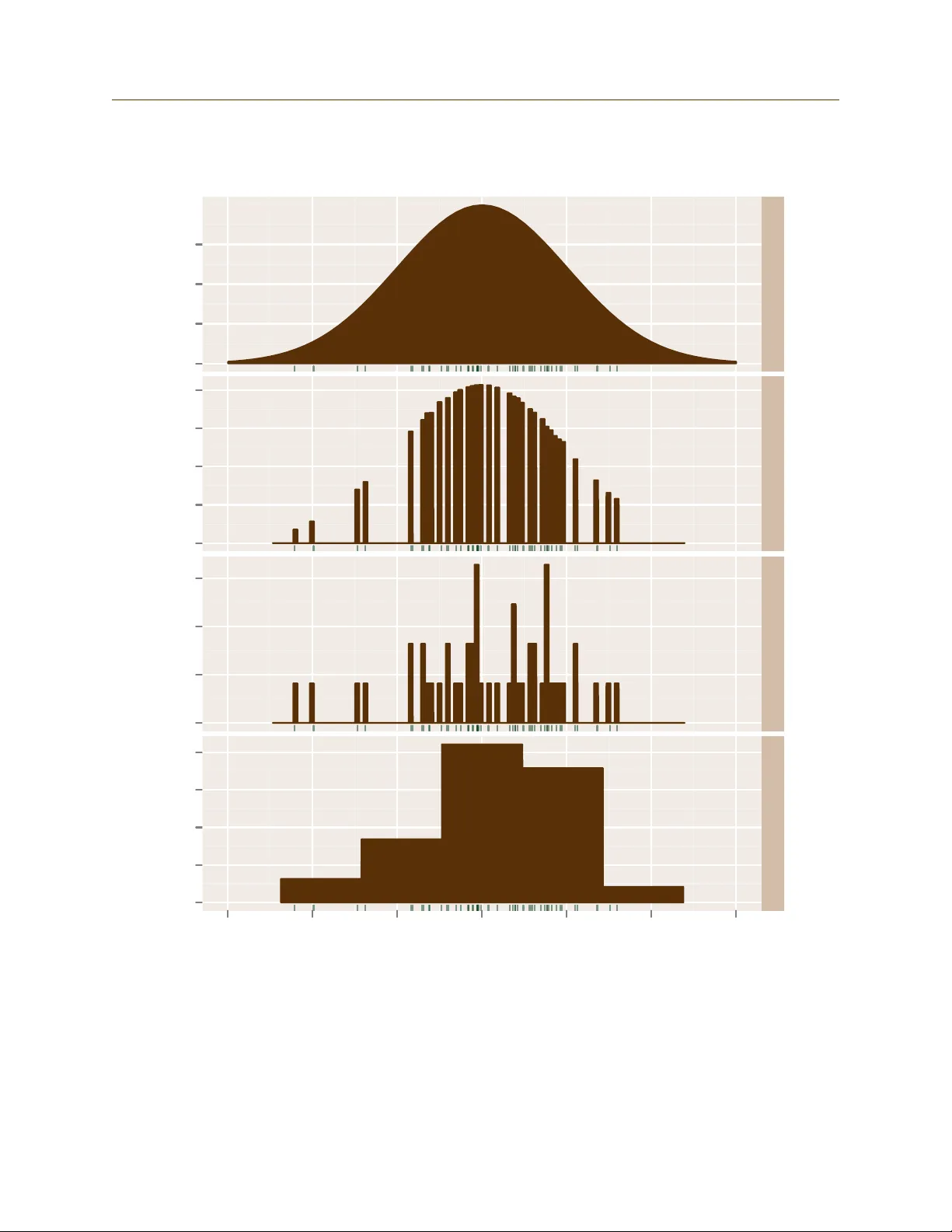
Marginal Lik eliho o d Estimation via Arrogance Sampling By Benedict Escoto Abstract This pap er describes a metho d for estimating the marginal lik eliho od or Bay es fac- tors of Ba y esian mo dels using non-paramet ric imp ortance sampling ( “arrogance sam- pling” ). This metho d can al so b e used to comp ute the normalizing constan t of probabil- it y distributions. Because the required inputs are samples from the distribution to b e normalized and the scaled densit y at those samples, this metho d may b e a conv enien t replacemen t for the harmonic mean estimator. The metho d has b een implemented in the open source R pac k age margLikArrogance . 1 In tro duction When a Ba y esian ev aluates t w o comp eting mo dels or theories, T 1 and T 2 , having observ ed a v ector of observ ation s x , Ba y es’ Theorem determines the p osterior ratio of the mo dels’ probabilities: p ( T 1 | x ) p ( T 2 | x ) = p ( x | T 1 ) p ( x | T 2 ) p ( T 1 ) p ( T 2 ) . (1) The quan tit y p ( x | T 1 ) p ( x | T 2 ) is called a Bayes factor and the quanti ties p ( x | T 1 ) and p ( x | T 2 ) are called the theories’ mar ginal likeliho o ds . The t yp es of Bay esian models considered in this paper ha ve a fixed finite num b er of parameters, each with their o wn probability function. If θ are parameters for a mo del T , then p ( x | T ) = Z p ( x | θ , T ) p ( θ | T ) d θ = Z p ( x ∧ θ | T ) d θ (2) Unfortunately , this integral is difficult to compute in practice. The purp ose of this pap er is to describ e one metho d for estimating it. Ev aluating in tegral (2) is sometimes called the problem of computing normalizing con- stan ts. The follo wing formula sho ws ho w p ( x | T ) is a normalizing constan t. p ( θ | x , T ) = p ( θ ∧ x | T ) p ( x | T ) (3) Th us the marginal lik eliho od p ( x | T ) is also the normalizing constan t of the p osterior pa- rameter distribution p ( θ | x , T ) assuming we are giv en the density p ( θ ∧ x | T ) whic h is often easy to compute in Ba y esian mo dels. F urthermore, Ba yesian statisticians t ypically pro duce samples from the posterior parameter distribution p ( θ | x , T ) even when not concerned with theory c hoice. In these case, computing the marginal likelihoo d is equiv alen t to computing 1 2 REVIEW OF LITERA TURE the normalizing constant of a distribution from which samples and the scaled density at these samples are a v ailable. The metho d describ ed in this pap er tak es this approac h. 2 Review of Literature Giv en ho w basic (1) is, it is p erhaps surprising that there is no easy and definitiv e wa y of applying it, ev en for si mple models. F urthermore, as the dimensionalit y and complexit y of probability distributions increase, the difficulty of appro ximation also increases. The follo wing three tec hniques for computing bay es factors or marginal likelihoo ds are imp ortan t but will not b e mentioned further here. 1. Analytic asymptotic approximatio ns suc h as Laplace’s metho d, see for instance Kass and Raftery (1995), 2. Bridge sampling/path sampling/thermodynamic in tegration (Gelman and Meng, 1998), and 3. Chib’s MCMC appro ximation (Chib, 1995; Chib and Jeliazk o v, 2005). Kass and Raftery (1995) is a p opular ov erview of the earlier literature on Bay es factor computation. All these metho ds can b e v ery successful in the righ t circumstances, and can often handle problems to o complex for the metho d describ ed here. Ho wev er, the metho d of this pap er may still b e useful due to its conv enience. The rest of section 2 describ es three approac hes that are relev an t to this paper. 2.1 Imp ortance Sampl ing Imp ortance sampling is a techni que for reducing th e v ariance of monte carlo in tegration. This section will note some general facts; see Ow en and Zhou (1998) for more information. Supp ose we are trying to compute the (p ossibly m ultidimensional) integral I of a w ell- b eha v ed function f ( θ ). Then I = Z f ( θ ) d θ = Z f ( θ ) g ( θ ) g ( θ ) d ( θ ) so if g ( θ ) is a probabilit y densit y function and θ i are indep enden t samples from it, then I = E g [ f ( θ ) /g ( θ )] ≈ 1 n n X i =1 f ( θ i ) g ( θ i ) = I n . (4) I n is an unbiased appro ximation to I and by the cen tral limit theorem will tend to a normal distribution. It has v ariance 2 2.2 Nonparametric Imp ortance Sampling 2 REVIEW OF LITERA TURE V ar[ I n ] = 1 n Z  f ( θ ) g ( θ ) − I  2 g ( θ ) d θ = 1 n Z ( f ( θ ) − I g ( θ )) 2 g ( θ ) d θ (5) Sometimes f is called the tar get and g is called the pr op osal distri bution. Assuming that f is non-negative, then minim um v ariance (of 0!) is ach iev ed when g = f /I —in other w ords when g is just the normalized version of f . This cannot b e done in practice b ecause normalizing f requires kno wing the quantit y I that we w an ted to approxi- mate; how ev er (5) is still imp ortan t b ecause it means that the more similar the proposal is to the target, the b etter our estimator I n b ecomes. In particular, f m ust go to 0 faster than g or the estimator will ha ve infinite v ariance. T o summarize this section: 1. Imp ortance sampling is a mon te carlo in tegration technique whic h ev aluates the target using samples from a proposal distribution. 2. The estimator is unbi ased, normally distributed, and its v ariance (if not 0 or infinit y) decreases as O ( n − 1 ) (using big- O notation). 3. The closer the prop osal is to the target, the b etter the estimator. The prop osal also needs to ha ve longer tails than the target. 2.2 Nonparametric Importance Sampling A difficulty with imp ortance sampling is that it is often difficult to choose a prop osal dis- tribution g . Not enough is known ab out f to choose an optimal distribution, and if a bad distribution is ch osen the result can ha v e large or ev en infinite v ariance. One approach to the selection of prop osal g is to use non-parametric techniques to build g from samples of f . I call this class of tec hniques self-imp ortance sampling, or arrogance sampling for short, b ecause they attempt to sample f from itself without using any external information. (And also isn’t it a bit arrogant to try to ev aluate a complex, multidimension al integral using only the v alues at a few p oin ts?) The metho d of this pap er falls in to this class and particularly deserv es the name because the target and prop osal (when they are b oth non-zero) ha v e exactly the same v alues up to a m ultiplicativ e constan t. Tw o pap ers whic h apply nonparametric imp ortance sampling to the problem of marginal lik eliho o d computati on (or computation of normalizing constan ts) are Zhang (1996) a nd Neddermey er (2009). Although both authors apply t heir m etho ds to more general situatio ns, here I will use the framew ork suggested b y (3) and assume that w e can comp ute p ( θ ∧ x | T ) for arbitrary θ and also that we can sample from the posterior parameter distribution p ( θ | x , T ). The goal is to estimate the normalizing constan t, the marginal lik eliho od p ( x | T ). Zhang’s approac h is to build the prop osal g using traditional k ernel densit y estimation. m samples are first dra wn from p ( θ | x , T ) and used to construct g . Then n samples are dra wn from g and used to ev aluate p ( x | T ) as in traditional imp ortance sampling. This approac h 3 2.3 Harmonic Mean Estimator 2 REVIEW OF LITERA TURE is quite intuit iv e b ecause k ernel estimation is a p opular w ay of appro ximating an unkno wn function. Zhang prov es that the v ariance of his estimator decreases as O ( m − 4 4+ d n − 1 ) where d is the dimensionalit y of θ , compared to O ( n − 1 ) for standard (parametric) importance sampling. There were, ho w ever, a few issues with Zhang’s metho d: 1. A k ernel densit y estim ate is equal to 0 at p oin ts far from the points the k ernel estimator w as built on. This is a problem b ecause imp ortance sampling requires the prop osal to ha ve longer tails than the target. This fact forces Zhang to mak e the restrictiv e assumption that p ( θ | x , T ) has compact support. 2. It is hard to compute the optimal kernel bandwidth. Zhang recommends using a plug-in estimator b ecause the function p ( θ ∧ x | T ) is av ailable, whic h is un usual for k ernel estimation problems. Sti ll, bandwidth selection app ears to require significan t additional analysis. 3. Finally , although the v ariance ma y decrease as O ( m − 4 4+ d n − 1 ) as m increases, the diffi- cult y of computing g ( θ ) also increases with m , b ecause it requires searc hing through the m basis p oin ts to find all the p oin ts close to θ . In m ultiple dimensions, this prob- lem is not trivial and may outw eigh the O ( m − 4 4+ d ) speedup (in the w orst case, practical ev aluation of g ( θ ) at a single p oin t may b e O ( m )). See Zlo c hin and Baram (2002) for some discussion of these issues. Neddermey er (2009) uses a similar approac h to Zhang and also ac hieves a v ariance of O ( m − 4 4+ d n − 1 ). It impro ves on Zhang’s approac h in tw o w ays relev an t to this pap er: 1. The supp ort of p ( θ | x , T ) is not required to b e compact. 2. Instead of using k ernel densit y estimators, linear blend frequency p olynomials (LBFPs) are used instead. LBFPs are basically histograms whose densit y is in terp olated b et w een adjacen t bins. As a result, the computation of g ( θ ) requires only finding which bin θ is in, and lo oking up the histogram v alue at that and adjacent bins (2 d bins in total). As we will see in section 3, the arrogance sampling described in this pap er is similar to the metho ds of Zhang and Neddermey er. 2.3 Harmonic Mean Estimator The harmonic mean estimator is a simple and notorious metho d for calculating marginal lik eliho o ds. It is a kind of imp ortance sampling, except the prop osal g is actually the distribution p ( θ | x , T ) = p ( θ ∧ x | T ) /p ( x | T ) to b e normalized and the target f is the kno wn distribution p ( θ | T ). Then if θ i are samples from p ( θ | x, T ), we apparen tly ha ve 4 3 DESCRIPTION OF TECHNIQUE 1 ≈ 1 n n X i =1 p ( θ i | T ) p ( θ i | x , T ) = 1 n n X i =1 p ( θ i | T ) p ( x | θ i , T ) p ( θ i | T ) /p ( x | T ) = 1 n n X i =1 1 p ( x | θ i , T ) /p ( x | T ) hence p ( x | T ) ? ≈ 1 n n X i =1 1 p ( x | θ i , T ) ! − 1 (6) Tw o adv an tages of the harmonic mean estimator are that it is simple to compute and only dep ends on samples from p ( θ | x, T ) and the likeli ho od p ( x | θ , T ) at those samples. The main dra wbac k of the harmonic mean estimator is that it do esn’t work—as mentioned earlier the imp ortance sampling prop osal distribution needs to hav e longer tails than the target. In this case the target p ( θ | T ) t ypically has longer tails than the prop osal p ( θ | x , T ) and th us (6) has infinite v ariance. Despite not working, the harmonic mean estimator contin ues to b e p opular (Neal, 2008). 3 Description of T ec hnique This pap er’s arrogance sampling technique is a simple method that applies the nonparametric imp ortance techni ques of Zhang and Neddermey er in an attempt to dev elop a metho d almost as conv enien t as the harmonic mean estimator. The only required inputs are samples θ i from p ( θ | x , T ) and the v alues p ( θ i ∧ x | T ) = p ( x | θ i , T ) p ( θ i | T ). This is similar to the harmonic mean estimator, but p erhaps sligh tly less con venien t because p ( θ i ∧ x | T ) is required instead of p ( x | θ i , T ). There are t wo basic steps: 1. T ake m samples from p ( θ | x , T ) and using mo dified histogram densit y estimation, con- struct probabilit y density function f ( θ ). 2. With n more samples from p ( θ | x , T ), estimate 1 /p ( x | T ) via importance sampling with target f and prop osal p ( θ | x , T ). These steps are describ ed in more detail below. 3.1 Construction of the Histogram Of the N total samples θ i from p ( θ | x , T ), the first m will b e used to mak e a histogram. The optimal c hoice of m will b e discussed b elo w, but in practice this seems difficult to determine. An arbitrary rule of min(0 . 2 N , 2 √ N ) can b e used in practice. 5 3.2 Imp ortance Sampling 3 DESCRIPTION OF TECHNIQUE With a traditional histogram, the only a v ailable information is the lo cation of the sampled p oin ts. In this case we also kno w the (scaled) heigh ts p ( θ ∧ x | T ) at eac h sampled p oin t. W e can use this extra information to impro v e the fit. Our “arrogan t” histogram f is constructed th e same as a regular hi stogram, except the bin heigh ts are not determined b y the n um b er of p oin ts in eac h bin, but rather by the minim um densit y o ver all points in the bin. If a bin con tains no sampled p oin ts, then f ( θ ) = 0 for θ in that bin. Then f is normalized so that R f ( θ ) d θ = 1. T o determine our bin width, w e can simply and somewhat arbitrarily set our bin width h so that the histogram is positive for 50% of the sampl ed points from the distribution p ( θ | x , T ). T o appro ximate h , w e can use a small num b er of samples (sa y , 40) from p ( θ | x , T ) and set h so that f ( θ ) > 0 for exactly half of these samples. Figure 1 compares the traditional and new histograms for a one dimensional normal distribution based on 50 samples. The green rug lines indicate the 50 sampled p oin ts whic h are the same for all. The arrogant histogram’s bin width is c hosen as ab o v e. The traditional histogram’s optimal bin width w as determined b y Scott’s rule to minimize mean squared error. As the figure shows, the modified histogram is muc h smoother for a given bin width, so a smaller bin width can b e used. On the other hand, f will either equal 0 or ha v e ab out twice the original densit y at each p oin t, while the traditional histogram’s densit y is n umerically close to the original densit y . 3.2 Imp ortance Sampl ing The remaining n = N − m − 40 sampled p oin ts can b e used for imp ortance sampling. Using equation (4) with histogram f as our target and p ( θ | x , T ) as the prop osal, we ha v e 1 ≈ I n = 1 n n X i =1 f ( θ i ) p ( θ i | x , T ) = 1 n n X i =1 f ( θ i ) p ( θ i ∧ x | T ) /p ( x | T ) hence p ( x | T ) ≈ p ( x | T ) /I n = 1 n n X i =1 f ( θ i ) p ( θ i ∧ x | T ) ! − 1 = A n (7) T o underscore the self-important/arrogan t nature of this approximat ion A n , we can rewrite (7) as p ( x | T ) ≈ H 1 n n X i =1 min { p ( θ j ∧ x | T ) : θ j and θ j are in the same bin } p ( θ i ∧ x | T ) ! − 1 where H is the histogram normalizing constan t. This equation shows that all the v alues in the n umerator and the denominator of our importance sampling are from the same distribution p ( θ ∧ x | T ). 6 3.2 Imp ortance Sampling 3 DESCRIPTION OF TECHNIQUE x Probability Density 0.0 0.1 0.2 0.3 0.0 0.2 0.4 0.6 0.8 0.0 0.5 1.0 1.5 0.0 0.1 0.2 0.3 0.4 −3 −2 −1 0 1 2 3 Density Arrogant Histogram T raditional Histogr am T rad Hist (Optim um BW) Figure 1: Histogra m Comparison 7 4 V ALIDITY OF METHOD Note that the histogram f is the target of the imp ortance sampling and p ( θ ∧ x | T ) is the prop osal. This is backw ards from the usual sc heme where the unknown distribution is the target and the kno wn distribution is the prop osal. Instead here the unkno wn distribution is the proposal, as in the harmonic mean estimator (see Rob ert and W raith (2009) for another example of this.) As in sectio n 2.1, our approxi mation of p ( x | T ) − 1 tends to a normal distribution as n → ∞ b y the cen tral limit theorem. This fact can be used to estimate a confidence in terv al around p ( x | T ). 4 V alidit y of Metho d This section will inv estigate the p erformance of the metho d. First, note that this metho d is just an implemen tation of imp ortance sampling, so A − 1 n should conv erge to p ( x | T ) − 1 with finite v ariance as long as the prop osal densit y p ( θ | x , T ) exists and is finite and p ositiv e on the compact region where the target histogram densit y is p ositiv e. T o calculate the sp eed of con v ergence we will use equation (5) where f is the histogram, g ( θ ) = p ( θ | x , T ), and I = 1 b ecause the histogram has b een normalized. Unless otherwise noted, we will assume b elo w that g : R d → R is finite, twice differen tiable and p ositiv e, and that R k∇· g ( θ ) k 2 g ( θ ) d θ is finite. 4.1 Histogram Bin Width One imp ortan t issue will b e ho w quick ly the d -dimensional histogram’s selected bin width h go es to 0 as the num b er of samples m → ∞ . This section will only offer an in tuitiv e argumen t. F or an y m , the histogram will enclose ab out the same probabilit y ( 1 2 ) and will ha ve ab out the same a v erage density in a fixed region. Eac h bin has volume h d , so if l is the n umber of bins then l h d = O (1) and h ∝ l − d . F urthermore, the distribution of the sampled p oin ts conv erges to the actual distribution g ( θ ). If m > O ( l ), an un b ounded num b er of sampled p oin ts w ould end up in each bin. If m < O ( l ), then some bins w ould ha ve no p oin ts in them. Neither of these is p ossible because exactly one sampled p oin t is necessary to establish eac h bin. Th us m ∝ l and h ∝ m − d . 4.2 Conditional V ariance Before estimating the conv ergence rate of A n w e will prov e something ab out the conditional v ariance of importance sampling. Let A = { θ : f ( θ ) > 0 } , 1 A b e the characteristic function of A , and q = R A g ( θ ) d θ . Define g A ( θ ) =  g ( θ ) /q if θ ∈ A 0 otherwise 8 4.3 Imp ortance Sampling Con v ergence 4 V ALIDITY OF METHOD Then g A is the density of g conditional on f > 0. Define V ar A and E A to mean the v ariance and exp ectation conditional on f ( θ ) > 0. Th us V ar( f ( θ ) /g ( θ )) = V ar(E( f ( θ ) /g ( θ ) | 1 A )) + E(V ar( f ( θ ) /g ( θ ) | 1 A )) = V ar  E A ( f ( θ ) /g ( θ )) if θ ∈ A 0 otherwise  + E  V ar A ( f ( θ ) /g ( θ )) if θ ∈ A 0 otherwise  = V ar  1 /q if θ ∈ A 0 otherwise  + q V ar A ( f ( θ ) /g ( θ )) = (1 /q ) 2 q (1 − q ) + 1 q V ar A ( f ( θ ) /q g ( θ )) = 1 − q q + 1 q V ar A ( f ( θ ) /g A ( θ )) W e will assume below that q = 1 2 , so that V ar( f ( θ ) /g ( θ )) = 1 + 2V ar A ( f ( θ ) /g A ( θ )) (8) 4.3 Imp ortance Sampl ing Con v ergence With f , g , and A as defined ab o v e, f and g A ha ve the same domain. Assuming errors in estimating q and normalization errors are of a lesser order of magnitude, we can treat the histogram heigh ts as b eing sampled from g A . Supp ose the histogram has l bins { B j } , each with width h and based around the p oin ts g A ( θ j ). Then b y equation (5), V ar A ( f ( θ ) /g A ( θ )) = l X j =1 Z B j ( f ( θ ) − g A ( θ )) 2 g A ( θ ) d θ = l X j =1 Z B j ( g A ( θ ) + ∇ g A ( θ ) · ( θ j − θ ) + O (( θ j − θ ) 2 ) − g A ( θ )) 2 g A ( θ ) d θ = l X j =1 Z B j ( ∇ g A ( θ ) · ( θ j − θ )) 2 + O (( θ j − θ ) 3 ) g A ( θ ) d θ ≤ l X j =1 Z B j k∇ · g A ( θ ) k 2 h 2 g A ( θ ) d θ = h 2 Z k∇ · g A ( θ ) k 2 g A ( θ ) d θ 9 5 IMPLEMENT A TION ISSUES Because h ∝ m − d where d is the n umber of dimensions, and m is the n um b er of samples used to mak e the histogram, V ar A ( f ( θ ) /g A ( θ )) ≤ C m − 2 /d where C ∝ R k∇· g A ( θ ) k 2 g A ( θ ) d θ . Putting this together with (8), we get V ar( I n ) = V a r( p ( x | T ) / A n ) = n − 1 (1 + O ( C m − 2 /d )) (9) 5 Implemen tation Issues 5.1 Sp eed of Con v ergence The v ariance of n − 1 (1 + O ( C m − 2 /d )) giv en b y (9) is asymptotically equal to n − 1 , which is the t ypical imp ortance sampling rate. In practice how ev er, the asymptotic results cannot distinguish useful from impractical estimators. If C m − 2 /d is small and V ar( p ( x | T ) / A n ) ≈ n − 1 , then p ( x | T ) can b e appro ximated in only 1000 samples to ab out 6% = 1 . 96 √ 1000 with 95% confidence. F or man y theor y c hoice purposes, this is quite sufficien t. Thus in t ypical problem cases the factor of C m − 2 /d will b e very significan t. If C m − 2 /d  1, then the conv ergence rate may in practice b e similar to n − 1 m − 2 /d . Compare this to the rate of n − 1 m − 4 / (4+ d ) for the metho ds prop osed by Zhang and Neddermey er. This metho d also uses simple histograms, instead of a more sophisticated density es- timation metho d (Zhang uses k ernel estimation, Neddermey er uses linear blend frequency p olynomial s). Although simple histograms conv erge slow er for large d as shown ab o v e, they are muc h faster to compute for large d . Neddermey er’s LBFP algorithm is quite efficient compared to Zhang’s, but its running time is O (2 d d 2 n d +5 d +4 ). d is a constant for any fixed problem, but if, sa y , d = 10, then the dimensionalit y constan t m ultiplies the running time b y 2 10 10 2 ≈ 10 5 . By con trast, this pap er’s metho d tak es only O ( dm log( m )) time to construct the initial histogram, and an additional O ( dn log( m )) time to do the imp ortance sampling. The main reason for the difference is that querying a simple histogram can be done in log( m ) time by computing the bin co ord inates and lo oking up the bin’s height in a tree structure. How ever, querying a LBFP requires blending all nearby bins and is thus exp onen tial in d . 5.2 When g = 0 Our discussion assumed that g ( θ ) = p ( θ | x , T ) w as alw ays p ositiv e. If g go es to 0 where the histogram is p ositiv e, the v ariance of A − 1 n will b e infinite. Ho wev er, this pap er’s metho d can still b e used if g ( θ ) is 0 o ver some well-defined area. 10 5.3 Bin Shap e 7 REFERENCES F or instance, supp ose one dimension θ k of p ( θ | T ) is defined b y a gamma distribution, so that p ( θ k | T ) = 0 if and only if θ k ≤ 0. Then we can ensure the v ariance is not infinite by c hec king that the histogram is only defined where θ k >  > 0 for some fixed  . The margLikArrogance pac k age con tains a simple mec hanism to do this. The user ma y sp ecify a range along eac h dimension of θ where it is kno wn that g > 0. If the histogram is non-zero outside of this range, the method ab orts with an error. Note that the v ariance of the estimator increases with R k∇· g A ( θ ) k 2 g A ( θ ) d θ . In practice the estimator will w ork well only when g do esn’t go to 0 to o quic kly where the histogram is p ositiv e. In these cases the histogram will b e defined w ell a wa y from any region where g = 0 and infinite v ariance w on’t b e an issue even if g = 0 somewhere. 5.3 Bin Shap e Cubic histogram bins were used ab o ve—their widths w ere fixed at h in eac h dimension. Al- though the asymptotic results aren’ t a ffected b y the shap e of eac h bin, for usable con vergence rates the bins’ dimensions need to compatible with the shap e of the high probabilit y region of p ( θ | x , T ). Unfortunately , it is difficult to determine the b est bin shap es. The margLikArrogance pack age contain s a simple work ar ound: b y default the distribu- tion is first scaled so that the sampled standard deviation along eac h dimension is constant. This is equiv alen t to setting each bin’s width b y dimension in prop ortion to that dimension’s standard deviati on. If thi s simple rule of thum b is insufficien t, the user ca n scale th e sampled v alues of p ( θ | x , T ) man ually (and make the corresp onding adjustmen t to the estimate A n ). 6 Conclusion This pap er has describ ed an “arrogance sampl ing” tec hnique for computing the marginal lik eliho o d or Bay es factor of a Ba y esian mo del. It in volv es using samples from the mo del’s p osterior parameter distribution along with the scaled v alues of the distribution’s density at those p oin ts. These samples are divided in to tw o main groups: m samples are used to build a histogram; n are used to imp ortance sample the histogram using the p osterior parameter distribution as the prop osal. This metho d is simple to implement and runs quickly in O ( d ( m + n )log( m )) time. Its asymptotic con v ergence rate, n − 1 (1 + O ( C m − 2 /d )), is not remark able, but in practice con- v ergence is fast for man y problems. Because the required inputs are similar to those of the harmonic mean estimator, it may b e a con venien t replacemen t for it. 7 References 1. S. Chib. “Marginal Lik eliho o d from the Gibbs Output” Journal of the Americ an Sta- tistic al Asso ciation . V ol 90, No 432. (1995) 11 7 REFERENCES 2. S. Chib and I. Jeliazk ov. “Accept-reject Metrop olis-Hastings sampling and marginal lik eliho o d estimation” Statistic a Ne erlandic a . V ol 59, No 1. (2005) 3. A. Gelman and X. Meng. “Simulating Normalizing Constants: F rom Importance Sam- pling to Bridge Sampling to P ath Sampling” Statistic al Scienc e . V ol 13, No 2. (1998) 4. R. Kass and A. Raftery . “Ba yes F actors” Journal of the Americ an Statistic al Asso cia- tion . V o l 90, No 430. (1995) 5. R. Neal. “The Harmonic Mean of the Lik eliho od: W orst Mon te Carlo Metho d Ever” . Blog p ost, http://radfordneal.wordpress.com/2008/08/17/the-harmonic-mean- of-the-likelihood-worst-monte-carl o-method-ever/ . (2008) 6. J. Neddermey er. “Computationally Efficient Nonparametric Imp ortance Sampling” Journal of the Americ an Statistic al Asso ciation . V ol 104, No 486. (2009) 7. A. Owen and Y. Zhou. “Safe and effective imp ortance sampling” Journal of the A mer- ic an Statistic al Asso ciation . V ol 95, No 449. (2000) 8. C. Robert and D. W rait h. “Computational metho ds for Ba y esian mo del choice” 9. P . Zhang. “Nonparametric Imp ortance Sampling” Journal of the Americ an Statistic al Asso ciation . V ol 91, No 435. (1996) 10. M. Zlo c hin and Y. Baram. “Efficien t Nonparametric Importance Sampling for Ba y esian Inference” Pr o c e e dings of the 2002 International Joint Confer enc e on Neur al Networks 2498–2502. (2002) 12