Valued Ties Tell Fewer Lies: Why Not To Dichotomize Network Edges With Thresholds

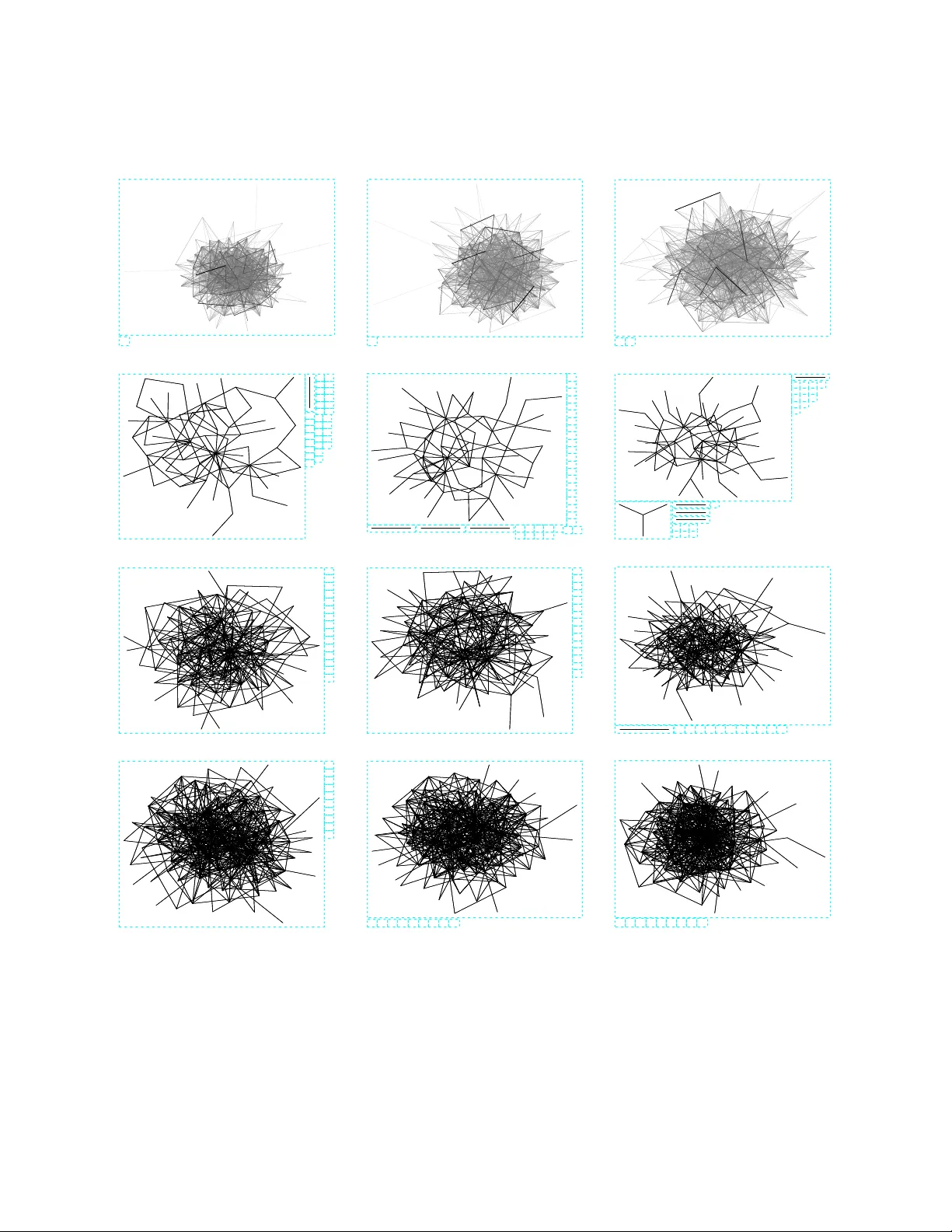
V alued Ties T ell F ew er Lies: Wh y Not T o Dic hotomize Net w ork Edges With Thresholds ∗ Andrew C. Thomas † Joseph K. Blitzstein ‡ Ma y 28, 2018 Abstract In order to conduct analyses of net work ed systems where connections b et ween individuals tak e on a range of v alues – counts, contin uous strengths or ordinal rankings – a common tec hnique is to dic hotomize the data according to their p ositions with respect to a threshold v alue. Ho wev er, there are t wo issues to consider: ho w the results of the analysis dep end on the choice of threshold, and what role the presence of noise has on a system with resp ect to a ﬁxed threshold v alue. W e show that while there are principled criteria of k eeping information from the v alued graph in the dichotomized version, they produce such a wide range of binary graphs that only a fraction of the relev ant information will be k ept. Additionally , while dic hotomization of predictors in linear models has a known asymptotic eﬃciency loss, the same pro cess applied to netw ork edges in a time series mo del will lead to an eﬃciency loss that grows larger as the netw ork increases in size. 1 In tro duction As the ma jority of publication in relational data and complex netw orks has deriv ed from the graph-theoretic framew ork, nearly all of the supp orting analytical to ols that ha ve been developed are meant to handle binary data input. As a result, there has b een a strong tendency to wards the transformation of v alued data in to the binary framework in order to conduct an analysis on the ensemble with particular attention to the individual no des. This is most often accomplished at the analysis stage through the dichotomization pro cedure: choose a threshold v alue, set all ties with equal or higher v alues to equal one, and all low er to equal zero. 1 ∗ Previous v ersions carried the title “The Thresholding Problem: Uncertain ties Due T o Dichotomization of V alued Ties”. † Visiting Assistan t Professor, Department of Statistics, Carnegie Mellon Universit y . Corresp onding author: email act@acthomas.ca. This w ork w as supp orted by gran t PO1-AG031093 from the NIA through the Christakis lab at Harv ard Medical Sc ho ol and D ARP A gran t 21845-1-1130102 through the CMU Statistics Departmen t. Thanks to attendees at the SAMSI Complex Net w orks W orkshop, the CMU CASOS Netw ork Science Group and the RAND Statistics Group for commen ts on earlier editions of this work. ‡ Assistan t Professor, Department of Statistics, Harv ard Universit y . 1 Dic hotomization is also kno wn as compression and slicing [Scott, 2000] throughout the literature, and across those disciplines that inv estigate netw orks. In previous versions of this work, we referred to the pro cedure as “thresholding”; we now use this term to refer only to the censoring of tie v alues b elow the threshold, and not the ﬁnal dichotomization. 1 The tendency to dichotomize has b een ab etted by the simplicity of working with binary out- comes, as w ell as the visualization metho ds curren tly av ailable for graphs. A threshold may also b e chosen for the sake of parsimon y of analysis, since examining only strong ties simpliﬁes their role in the system under study . Additionally , limiting an analysis to the strongest ties that hold a net work together is p erceived to b e a mechanism for reducing noise that is seen to b e caused b y a larger num b er of weak er connections. This is certainly true when using standard algorithms for plotting a net work; an excess of ties on the prin ted page, with resp ect to the nodes of the system, will obscure other ties that may ha ve more meaning for the dynamics of the system. If the goal of dichotomization is to learn ab out the underlying v alued system, the outcome may b e diﬃcult to quantify . In particular, if the goal is to c ho ose a cut-p oint that is in some sense “optimal”, the metho d for c ho osing the cut should reﬂect a minimum loss of information from the v alued system. But if the quantit y of interest is not meaningful in the v alued case – for example, that all edges are non-zero but most are very small, so that the edge-count diameter of the system is 1 – then it may pro ve diﬃcult to choose a condition for optimality . There are man y diﬀerent classes of input data in the literature that are sub jected to di- c hotomization: • Correlation or partial correlation as evidence of net w ork ties (Achard et al. [2006], Section 7.3.2 in Kolaczyk [2009], Hidalgo et al. [2009]). Net work ties are elicited b y measuring the outcomes b etw een tw o no des o ver time or rep etitions, and the strength of correlation determines the existence of an underlying tie. • Count-incidence data (suc h as the EIES message data in F reeman and F reeman [1980]), where a connection v alue is the n umber of times t w o individuals are counted together, b e it comm unication, collab oration or attendance. More classes of coun t data in volving directed transactions are found in the agriculture literature [Ortiz-Pelaez et al., 2006; Robinson and Christley, 2007]. Choudh ury et al. [2010] considers the thresholding problem on mo dern electronic communication data sets and attempts the same type of pro cedure we endorse, but with the prediction of future b eha viour as the optimality criterion. A sp ecial case of coun t-incidence is the pro jection of a binary bipartite net work, in whic h there are t w o classes of no des that only hav e ties across groups, not within. One example of this is the netw ork of mem b erships of individuals in organizations, which can b e pro jected in to an organization-only netw ork with tie strength represen ting the n um b er of common individuals. In the case of a low-densit y netw ork, it may suﬃce to set the threshold at 1; ho wev er, this ma y still result in a signiﬁcan t loss of information. An example of a coun t model with noise is Figure 1. In this case, the c hosen threshold is the minimum v alue that main tains a giant comp onent, and the resulting top ology of the binary net w ork is ring-lik e. Ho wev er, for another netw ork generated from the same 2 True Distances ● ● ● ● ● ● ● ● ● ● ● ● ● ● ● ● ● ● ● ● ● ● ● ● ● ● ● ● ● ● ● ● ● ● ● ● ● ● ● ● ● ● ● ● ● ● ● ● ● ● ● ● ● ● ● ● ● ● ● ● ● ● ● ● ● ● ● ● ● ● ● ● ● ● ● ● ● ● ● ● ● ● ● ● ● ● ● ● ● ● ● ● ● ● ● ● ● ● ● ● 1 2 3 4 5 6 7 8 9 10 11 12 13 14 15 16 17 18 19 20 21 22 23 24 25 26 27 28 29 30 31 32 33 34 35 36 37 38 39 40 41 42 43 44 45 46 47 48 49 50 51 52 53 54 55 56 57 58 59 60 61 62 63 64 65 66 67 68 69 70 71 72 73 74 75 76 77 78 79 80 81 82 83 84 85 86 87 88 89 90 91 92 93 94 95 96 97 98 99 100 ● ● ● ● ● ● ● ● ● ● ● ● ● ● ● ● ● ● ● ● ● ● ● ● ● ● ● ● ● ● ● ● ● ● ● ● ● ● ● ● ● ● ● ● ● ● ● ● ● ● ● ● ● ● ● ● ● ● ● ● ● ● ● ● ● ● ● ● ● ● ● ● ● ● ● ● ● 1 2 3 4 5 6 7 8 9 10 11 12 13 14 15 16 17 18 19 20 21 22 23 24 25 26 27 28 29 30 31 32 33 34 35 36 37 38 39 40 41 42 43 44 45 46 47 48 49 50 51 52 53 54 55 56 57 58 59 60 61 62 63 64 65 66 67 68 69 70 71 72 73 74 75 76 77 78 79 80 81 82 83 84 85 86 87 88 89 90 91 92 93 94 95 96 97 98 99 100 Observed Distances ● ● ● ● ● ● ● ● ● ● ● ● ● ● ● ● ● ● ● ● ● ● ● ● ● ● ● ● ● ● ● ● ● ● ● ● ● ● ● ● ● ● ● ● ● ● ● ● ● ● ● ● ● ● ● ● ● ● ● ● ● ● ● ● ● ● ● ● ● ● ● ● ● ● ● ● 1 2 3 4 5 6 7 8 9 10 11 12 13 14 15 16 17 18 19 20 21 22 23 24 25 26 27 28 29 30 31 32 33 34 35 36 37 38 39 40 41 42 43 44 45 46 47 48 49 50 51 52 53 54 55 56 57 58 59 60 61 62 63 64 65 66 67 68 69 70 71 72 73 74 75 76 77 78 79 80 81 82 83 84 85 86 87 88 89 90 91 92 93 94 95 96 97 98 99 100 Figure 1: A demonstration of when dic hotomization can give an extremely misleading picture of an underlying system. Upper left: a 100-no de netw ork with ring-t yp e top ology and integer- v alued ties, pro duced from a generative mo del with P oisson-type edge v alues. Upp er righ t: a dic hotomized v ersion of this graph with a cut-p oint c hosen to maintain the giant comp onen t. Belo w: a dic hotomized v ersion of a graph from the same generativ e family with the identical cut- p oin t v alue. Note that the top ological discrepancy , due to the underlying random pro cess go v erning the strengths of ties, can p oten tially mislead an in vestigator on the nature of the connected system. F or example, no de 18 is located on the ring in the ﬁrst case, and therefore considerably more cen tral, than in the second case while on the p eriphery . 3 underlying mo del, that same c hoice of threshold creates an line-lik e binary graph, which has v ery diﬀeren t topological properties – among others, it has double the diameter. This is mean t to illustrate that if the inten t of dichotomization is to reduce noise b y simplifying the structure of the system, the choice of threshold may ha ve exactly the opp osite eﬀect. • Categorical/ordinal data on relationship t yp e (the EIES acquaintance data in F reeman and F reeman [1980]). In this case, the ordinal data represent the strength of an asso ciation b et ween t wo p eople as rep orted in qualitative fashion, such as { “nev er heard of them”, “acquain tances”, “casual friends”, “b est friends” } and subsequent analysis is p erformed by forming tw o groups. • Rank data such as in [Newcom b, 1961], in which resp onden ts w ere asked to iden tify their order of preference for eac h other mem b er in the study o ver a p erio d of sev eral mon ths. This is diﬀeren t from the previous cases since the actual underlying relationships can v ary greatly; a p erson in a tight group of 4 likely has v ery diﬀerent feelings for their assignment of “third-b est friend” than someone in a tight group of 3, whose third choice lies outside their immediate so cial sphere. Thresholds can b e tak en on an individual’s preferences alone, or whether tw o individuals m utually ranked the other highly . (Note: the former is also another case of the degree- censoring problem, discussed in detail in ? .) W e b egin with a discussion of v arious motiv ations for dichotomizing a v alued data set, and then reviewing w ork on the consequences of dichotomizing data in the linear mo delling literature, and under what circumstances it is maximally eﬃcien t. F ollowing this background review, the eﬀect of dichotomization on the geometric summaries of the net work is discussed, ﬁrst through the simulation of v arious families of v alued tie strengths under the GLM framework, then on three real examples from the literature. This is follo wed by an in vestigation the c hoice of threshold on a no dal outcome when the tie is a part of a predictor in a linear mo del, demonstrate a considerable loss of eﬃciency as compared to the linear v alued case in simulated examples, and show that the co verage probabilities for conﬁdence/probabilit y interv als can b e considerably distorted. The c hapter concludes with a discussion on the use of dic hotomization in general, with recommendations regarding its use in net w ork problems. 2 Motiv ations for Dic hotomization There are several reasons wh y the dichotomization procedure is app ealing in an inv estigation aside from conv enience and simplicity . Here are several classes of motiv ation that are of particular in terest. 4 • Use of Exclusiv ely Binary Metho ds . Sev eral classes of mo dels hav e b een designed to incorp orate binary information directly , including the exp onen tial random graph mo del (ER GM or p-star; see ? for an introduction), whose inputs are often summary statistics of coun ts of top ological features, and the W atts-Strogatz small-world [ ? ] and Barabasi-Alb ert preferen tial attac hment mo dels [ ? ] whose generativ e mec hanisms are binary in nature, and also enjoy a large record of veriﬁcation across many disciplines. No less relev ant are our p erceptions on the degrees of separation betw een individuals in a connected system; a friend of a friend is a well-deﬁned notion, whereas a low-strength connection one step a wa y ma y not b e easy to compare to the inﬂuence of an individual tw o very short steps aw a y . While it ma y be possible to reﬁne these mec hanisms to incorp orate weigh ted data, these mo diﬁcations ha ve not y et been veriﬁed or published and cannot b e relied up on in real- w orld case studies. As a result, the thresholding mec hanism is seen as a reasonable wa y of extracting information from a v alued data set for use in empirically v eriﬁed metho ds. • Ease of Input and Data Collection . The need to classify con tin uously-v alued quan tities in to a set of discrete groups is widespread throughout all of science and tec hnology , par- ticularly b ecause of the asso ciated need to make clear decisions based on this information, whether or not there is a distinct change in the b ehaviour of a system at the threshold level. F or example, a p erson is considered ob ese if their the b o dy-mass index (BMI) exceeds 30 2 , though there is no dramatic diﬀerence for t wo otherwise iden tical p eople whose BMIs are 29.5 and 30.5; it serv es as a useful b enc hmark for making medical decisions b y preserving a large piece of the information. In this w ay , the act of dic hotomization is more similar to the rounding of decimal places. Ho wev er, b y rounding to o early in the op eration, the error in tro duced will hav e more opp or- tunities to propagate and magnify through an analysis if not prop erly track ed. • Ease of Output in Graphical Represen tations . The visual app eal of graphs and net- w orks has contributed to muc h of the ﬁeld’s attention in the past decade. When plotting a graphical structure, with n no des and  n 2  undirected edges, it can quickly b ecome diﬃcult to visually disco v er the most relev an t no des or connections. A clever choice of threshold can illuminate which nodes are most central, whic h connections the most vital. • Sparsity of Structure . In data where there are v ery few natural zero es (if any), di- c hotomization provides a wa y to select for a small num b er of connections whic h are though t to b e of the greatest imp ortance to the system, or to nominate a num b er of ties for more in-depth study . This use, in particular, exempliﬁes the diﬀerence b et ween a “structural” zero, in which no tie exists, from a “signal” zero, in which the transmission along or activit y across a known tie is so small as to render it redundant to the op eration of the netw ork. 2 Source: WHO w ebsite. h ttp://apps.who.int/bmi/index.jsp?in troPage=in tro 3.h tml, accessed July 21, 2009. 5 • Binning T o Address Nonlinearit y and Reduce Noise . A quan tit y that appears to ha ve a linear eﬀect on a short range of scale ma y behav e quite diﬀeren tly o ver larger scales. 3 If there is a nonlinear relationship in the data, binning the data in to distinct ordinal categories has man y adv an tages, namely , the reduction of total mean-squared error, and a corresp onding increase in p ow er for detecting a true non-zero relationship o ver an improp erly sp eciﬁed linear analysis. By restricting the n umber of bins to tw o, the in vestigator ma y b e imp osing a stricter condition on the data than is necessary . Eac h case has its merits. The ﬁrst is indisputable, in that binary-v alued metho ds require binary-v alued input. When dichotomization is conducted at the analysis stage, the data collection question is mo ot; how ever, if done at the design stage, as in a survey or sampling study , the impact is done and the eﬀect must b e considered in the analysis. It is diﬃcult to measure the app eal of a graphical displa y in quantitativ e terms, though there are visual characteristics that ma y b e apparent in statistical summaries that can b e discov ered. As for binning, it is one of a large num b er of data transformation metho ds that can b e p erformed to address nonlinearit y and noise, and a subset of general categorization, whic h is b eyond the scop e of this c hapter. 3 Bac kground on Dic hotomization Metho ds Dic hotomization of netw ork ties is often an ad ho c pro cedure. By exp erimen ting with v arious cutoﬀ p oin ts and examining the prop erties of the resulting net works, practitioners ma y choose an “appropriate” cut p oin t that purp ortedly captures the essence of a net work phenomenon. Here are metho ds that ha ve b een traditionally used to dichotomize data without the need for ad ho c standards. 3.1 Dic hotomization of Predictors in Linear Mo dels There are man y reasons why statistical practitioners might wish to take a quan titativ e or categor- ical v ariable and dichotomize it as an input for a standard linear regression. Principally is the ease of explanation and in terpretability of the diﬀerence b etw een a “high” and a “lo w” group, primarily for the ease of digestion for a la y audience. It is vitally imp ortan t to c ho ose an “optimal” cut-p oin t based on information provided by the predictor alone; to c ho ose a cut-p oin t that dep ends on the outcome leads to serious issues, the least of which b eing the inv alidity of the p-v alue for statisti- cal signiﬁcance [Royston et al., 2006] due to an innate m ultiple comparison b etw een all p ossible selections. It has b een noted for decades (see Kelley [1939] for a historical example) that by c ho osing a cut-p oin t at the middle, an in vestigator is selecting p oin ts for analysis near the cut-p oint that 3 An appropriate quote: “Money do esn’t alw ays buy happiness. P eople with ten million dollars are no happier than p eople with nine million dollars.” -Hobart Brown 6 are close together in the predictor but are radically separated as a result of dichotomization. It ma y make more sense to remov e the middle p oints from the analysis entirely; Gelman and P ark [2009] shows that c ho osing a trichotomization sc heme by k eeping those p oints in the upp er and lo wer thirds for a uniformly distributed co v ariate will maximize the resulting eﬃciency while still main taining in terpretability . Splitting the ties into three groups solves no problems for net work statistical measurement or for epidemiology . It may , how ever, pro ve to b e of some b eneﬁt in longitudinal mo del studies where the predictor is the lagged outcome of a neigh b ouring no de m ultiplied b y the tie strength; this is discussed in greater detail in Section 7. 3.2 Minimal “Gian t Comp onent” Metho ds The w ork of Erdos and Ren yi [1960] established the conditions under which an Erdos-Renyi random graph w ould con tain a “giant comp onent”, a subset of no des that are mutually reac hable through their connected edges; namely , that the probability of any particular edge existing multiplied b y the num b er of no des will tend to b e greater than 1. The sudden app earance of a gian t component with the adjustment of the allow ance threshold has b een lik ened to phase transition changes in matter, as well as p ercolation conditions on somewhat-regular lattices [Calla wa y et al., 2000]. The existence of a giant comp onen t in a graph has particular implications in epidemiological con texts; if no such comp onen t exists, there can b e no transmission along the graph. F rom this idea, the metho d of choosing a minimum threshold v alue for which a gian t comp onent emerges. If a net work is thought to b e minimally connected, it would pro vide a useful upp er b ound on the eﬀect of information transmission compared to lo wer thresholds. This cut-p oint is often taken where the net work is app earing to grow at its most rapid rate, meaning that the app earance of some nodes and edges o v er others ma y app ear to b e the product of an underlying noisy pro cess rather than the inclusion of links that are sp eciﬁcally resp onsible for the connectivit y of a system. How ev er, it also acts as a p oint of maxim um discrimination b etw een the full and empt y states, a natural t yp e of midp oin t b et w een extreme v alues, and therefore deserv es some attention. This metho d is also p opular for graphical purp oses as a wa y of presenting an uncluttered pro jection of the system in t wo dimensions (see Hidalgo et al. [2009, 2007] for examples). 4 Sim ulation Mo dels With the deﬁnition of Generalized Linear Models for v arious v alued net w ork c haracteristics, there is a basis for considering the eﬀect of dic hotomization, b oth at the selection of v arious cut p oints as well as across v arious instances of random v ariation. The following procedure is used for testing the eﬀect of dic hotomization: 7 • Select a generativ e family from the GLM to olkit where edges hav e nonnegativ e v alue: Y ij | µ ij ∼ 1 µ ij Gamma ( µ 2 ij ) and Y ij | µ ij ∼ P oisson ( µ ij ) are the tw o generativ e families used in this exp eriment. Note that the mean of the P oisson can v ary within a single run, leading to the ov erdisp ersion that c haracterizes the heterogeneity presen t in a Negative Binomial random v ariable. • Select a series of laten t parameters that deﬁne µ ij : – Sender/receiver eﬀects α i ∼ N (0 , σ 2 α ), where a larger σ α yields more heterogeneity b et ween no des. – Latent geometric structure: no des hav e p ositions ~ d i , and a co eﬃcient of distance vs. connectivit y γ . Nodes can lie equally spaced on a ring of unit radius, or in a single cloud from a biv ariate normal distribution. – Latent clusters. Each no de is assigned mem b ership in one of three clusters ( a i = k ), and prefer links either within their cluster or with those no des in other clusters with prop ensit y λ . In this sim ulation, only one of clusters and geometry can b e implemented at one time. – An assortativ e mixing factor χ equal to 0.5, 0 or -0.5 (the disassortativ e case). – The n umber of no des in the system. All together, this giv es an outcome parameter equal to µ ij = α i + α j + χα i α j − γ | ~ d i − ~ d j | + λ I ( a i = a j ); (1) a list of all options for the ab ov e parameters is sho wn in T able 1. T o keep the parameter v alues p ositiv e, their v alues are b ounded ab ov e zero with the trans- formation function µ pos = f ( µ ) = exp ( µ − 1) I ( µ < 1) + µ I ( µ ≥ 1), rather than setting all negativ e-parameter dra ws to zero; in execution, the diﬀerence is negligible when threshold v alues are ab ov e 1. 8 Quan tity V alues No des 50 100 200 300 400 500 600 P op/Greg Signal 0.1 0.5 1 2.5 10 100 Geometry None Ring Cloud Cluster + Cluster - Geo. Strength 0.25 3 Assortativ e Mixing 0 0.5 -0.5 F amily Gamma P oisson T able 1: Simulation parameters to inv estigate the eﬀects of dichotomization in v alued net works. F or the geometric measures, generated netw orks ha ve a maxim um size of 300; larger netw orks are implemen ted in Section 7, the consequences on linear mo dels using dic hotomized netw orks. • Select a “ladder” of threshold v alues, reﬂecting the c hanging density and connectivit y of the dic hotomized systems. These v alues may b e b est determined by ﬁrst considering the av erage n umber of edges p er no de and choosing the threshold that corresp onds to that fraction. • Given the selected generative mo del, pro duce a num b er of replicates of the v alued netw ork (10, for the purp oses of this analysis.) F or eac h replicate, create a series of binary net works using the threshold ladder. • Given c hosen conditions, compare prop erties of the sim ulated net w orks within a single v alued instance at all thresholds, taking the av erage across all instances at each threshold if p ossible (see Figure 2 for an example.) Giv en the run of these sim ulations, it remains to be demonstrated ho w to extract the maximum amoun t of information from a dic hotomized netw ork represen tation. Estimates obtained through the dichotomized net work must ha ve meaning in terms of the individuals within it. In the sections that follo w, three lev els of eﬀects are examined: static no de c haracteristics, net work diameter and dy adic causation. First, the problem of comparing quantities b et ween v alued graphs and their dic hotomized coun terparts in a physically v alid fashion is addressed. 4.1 V alid Estimation Through A Change of Units The v alues and weigh ts in relational data typically ha ve physical meaning. As a result, dic hotomiza- tion of data is essen tially a c hange of units from an observ ational measure into a friendship mea- sure, alb eit as a lossy many-to-one transformation. Quantities that are calculated under the dic hotomized structure will act as v alid estimators for the v alued quantities if units are accounted for. This is similar to the example set by Gelman and Park [2009], in which the eﬃciency of a predictor is compared b et ween the v alued and dichotomized cases. While the original measurement has its own scale in terms of a physical quantit y (n umber of comm unications, min utes in contact, etc.) there is rarely such a deﬁnition for the binary tie. In 9 ● ● ● ● ● ● ● ● ● ● ● ● ● ● ● ● ● ● ● ● ● ● ● ● ● ● ● ● ● ● ● ● ● ● ● ● ● ● ● ● ● ● ● ● ● ● ● ● ● ● ● ● ● ● ● ● ● ● ● ● ● ● ● ● ● ● ● ● ● ● ● ● ● ● ● ● ● ● ● ● ● ● ● ● ● ● ● ● ● ● ● ● ● ● ● ● ● ● ● ● 1 2 3 4 5 6 7 8 9 10 11 12 13 14 15 16 17 18 19 20 21 22 23 24 25 26 27 28 29 30 31 32 33 34 35 36 37 38 39 40 41 42 43 44 45 46 47 48 49 50 51 52 53 54 55 56 57 58 59 60 61 62 63 64 65 66 67 68 69 70 71 72 73 74 75 76 77 78 79 80 81 82 83 84 85 86 87 88 89 90 91 92 93 94 95 96 97 98 99 100 ● ● ● ● ● ● ● ● ● ● ● ● ● ● ● ● ● ● ● ● ● ● ● ● ● ● ● ● ● ● ● ● ● ● ● ● ● ● ● ● ● ● ● ● ● ● ● ● ● ● ● ● ● ● ● ● ● ● ● ● ● ● ● ● ● ● ● ● ● ● ● ● ● ● ● ● ● ● ● ● ● ● ● ● ● ● ● ● ● ● ● ● ● ● ● ● ● ● ● ● 1 2 3 4 5 6 7 8 9 10 11 12 13 14 15 16 17 18 19 20 21 22 23 24 25 26 27 28 29 30 31 32 33 34 35 36 37 38 39 40 41 42 43 44 45 46 47 48 49 50 51 52 53 54 55 56 57 58 59 60 61 62 63 64 65 66 67 68 69 70 71 72 73 74 75 76 77 78 79 80 81 82 83 84 85 86 87 88 89 90 91 92 93 94 95 96 97 98 99 100 ● ● ● ● ● ● ● ● ● ● ● ● ● ● ● ● ● ● ● ● ● ● ● ● ● ● ● ● ● ● ● ● ● ● ● ● ● ● ● ● ● ● ● ● ● ● ● ● ● ● ● ● ● ● ● ● ● ● ● ● ● ● ● ● ● ● ● ● ● ● ● ● ● ● ● ● ● ● ● ● ● ● ● ● ● ● ● ● ● ● ● ● ● ● ● ● ● ● ● ● 1 2 3 4 5 6 7 8 9 10 11 12 13 14 15 16 17 18 19 20 21 22 23 24 25 26 27 28 29 30 31 32 33 34 35 36 37 38 39 40 41 42 43 44 45 46 47 48 49 50 51 52 53 54 55 56 57 58 59 60 61 62 63 64 65 66 67 68 69 70 71 72 73 74 75 76 77 78 79 80 81 82 83 84 85 86 87 88 89 90 91 92 93 94 95 96 97 98 99 100 ● ● ● ● ● ● ● ● ● ● ● ● ● ● ● ● ● ● ● ● ● ● ● ● ● ● ● ● ● ● ● ● ● ● ● ● ● ● ● ● ● ● ● ● ● ● ● ● ● ● ● ● ● ● ● ● ● ● ● ● ● ● ● ● ● ● ● ● ● ● ● ● ● ● ● ● ● ● ● ● ● ● ● ● ● ● ● ● ● ● ● ● ● ● ● ● ● ● ● ● 1 2 3 4 5 6 7 8 9 10 11 12 13 14 15 16 17 18 19 20 21 22 23 24 25 26 27 28 29 30 31 32 33 34 35 36 37 38 39 40 41 42 43 44 45 46 47 48 49 50 51 52 53 54 55 56 57 58 59 60 61 62 63 64 65 66 67 68 69 70 71 72 73 74 75 76 77 78 79 80 81 82 83 84 85 86 87 88 89 90 91 92 93 94 95 96 97 98 99 100 ● ● ● ● ● ● ● ● ● ● ● ● ● ● ● ● ● ● ● ● ● ● ● ● ● ● ● ● ● ● ● ● ● ● ● ● ● ● ● ● ● ● ● ● ● ● ● ● ● ● ● ● ● ● ● ● ● ● ● ● ● ● ● ● ● ● ● ● ● ● ● ● ● ● ● ● ● ● ● ● ● ● ● ● ● ● ● ● ● ● ● ● ● ● ● ● ● ● ● ● 1 2 3 4 5 6 7 8 9 10 11 12 13 14 15 16 17 18 19 20 21 22 23 24 25 26 27 28 29 30 31 32 33 34 35 36 37 38 39 40 41 42 43 44 45 46 47 48 49 50 51 52 53 54 55 56 57 58 59 60 61 62 63 64 65 66 67 68 69 70 71 72 73 74 75 76 77 78 79 80 81 82 83 84 85 86 87 88 89 90 91 92 93 94 95 96 97 98 99 100 ● ● ● ● ● ● ● ● ● ● ● ● ● ● ● ● ● ● ● ● ● ● ● ● ● ● ● ● ● ● ● ● ● ● ● ● ● ● ● ● ● ● ● ● ● ● ● ● ● ● ● ● ● ● ● ● ● ● ● ● ● ● ● ● ● ● ● ● ● ● ● ● ● ● ● ● ● ● ● ● ● ● ● ● ● ● ● ● ● ● ● ● ● ● ● ● ● ● ● ● 1 2 3 4 5 6 7 8 9 10 11 12 13 14 15 16 17 18 19 20 21 22 23 24 25 26 27 28 29 30 31 32 33 34 35 36 37 38 39 40 41 42 43 44 45 46 47 48 49 50 51 52 53 54 55 56 57 58 59 60 61 62 63 64 65 66 67 68 69 70 71 72 73 74 75 76 77 78 79 80 81 82 83 84 85 86 87 88 89 90 91 92 93 94 95 96 97 98 99 100 ● ● ● ● ● ● ● ● ● ● ● ● ● ● ● ● ● ● ● ● ● ● ● ● ● ● ● ● ● ● ● ● ● ● ● ● ● ● ● ● ● ● ● ● ● ● ● ● ● ● ● ● ● ● ● ● ● ● ● ● ● ● ● ● ● ● ● ● ● ● ● ● ● ● ● ● ● ● ● ● ● ● ● ● ● ● ● ● ● ● ● ● ● ● ● ● ● ● ● ● 1 2 3 4 5 6 7 8 9 10 11 12 13 14 15 16 17 18 19 20 21 22 23 24 25 26 27 28 29 30 31 32 33 34 35 36 37 38 39 40 41 42 43 44 45 46 47 48 49 50 51 52 53 54 55 56 57 58 59 60 61 62 63 64 65 66 67 68 69 70 71 72 73 74 75 76 77 78 79 80 81 82 83 84 85 86 87 88 89 90 91 92 93 94 95 96 97 98 99 100 ● ● ● ● ● ● ● ● ● ● ● ● ● ● ● ● ● ● ● ● ● ● ● ● ● ● ● ● ● ● ● ● ● ● ● ● ● ● ● ● ● ● ● ● ● ● ● ● ● ● ● ● ● ● ● ● ● ● ● ● ● ● ● ● ● ● ● ● ● ● ● ● ● ● ● ● ● ● ● ● ● ● ● ● ● ● ● ● ● ● ● ● ● ● ● ● ● ● ● ● 1 2 3 4 5 6 7 8 9 10 11 12 13 14 15 16 17 18 19 20 21 22 23 24 25 26 27 28 29 30 31 32 33 34 35 36 37 38 39 40 41 42 43 44 45 46 47 48 49 50 51 52 53 54 55 56 57 58 59 60 61 62 63 64 65 66 67 68 69 70 71 72 73 74 75 76 77 78 79 80 81 82 83 84 85 86 87 88 89 90 91 92 93 94 95 96 97 98 99 100 ● ● ● ● ● ● ● ● ● ● ● ● ● ● ● ● ● ● ● ● ● ● ● ● ● ● ● ● ● ● ● ● ● ● ● ● ● ● ● ● ● ● ● ● ● ● ● ● ● ● ● ● ● ● ● ● ● ● ● ● ● ● ● ● ● ● ● ● ● ● ● ● ● ● ● ● ● ● ● ● ● ● ● ● ● ● ● ● ● ● ● ● ● ● ● ● ● ● ● ● 1 2 3 4 5 6 7 8 9 10 11 12 13 14 15 16 17 18 19 20 21 22 23 24 25 26 27 28 29 30 31 32 33 34 35 36 37 38 39 40 41 42 43 44 45 46 47 48 49 50 51 52 53 54 55 56 57 58 59 60 61 62 63 64 65 66 67 68 69 70 71 72 73 74 75 76 77 78 79 80 81 82 83 84 85 86 87 88 89 90 91 92 93 94 95 96 97 98 99 100 ● ● ● ● ● ● ● ● ● ● ● ● ● ● ● ● ● ● ● ● ● ● ● ● ● ● ● ● ● ● ● ● ● ● ● ● ● ● ● ● ● ● ● ● ● ● ● ● ● ● ● ● ● ● ● ● ● ● ● ● ● ● ● ● ● ● ● ● ● ● ● ● ● ● ● ● ● ● ● ● ● ● ● ● ● ● ● ● ● ● ● ● ● ● ● ● ● ● ● ● 1 2 3 4 5 6 7 8 9 10 11 12 13 14 15 16 17 18 19 20 21 22 23 24 25 26 27 28 29 30 31 32 33 34 35 36 37 38 39 40 41 42 43 44 45 46 47 48 49 50 51 52 53 54 55 56 57 58 59 60 61 62 63 64 65 66 67 68 69 70 71 72 73 74 75 76 77 78 79 80 81 82 83 84 85 86 87 88 89 90 91 92 93 94 95 96 97 98 99 100 ● ● ● ● ● ● ● ● ● ● ● ● ● ● ● ● ● ● ● ● ● ● ● ● ● ● ● ● ● ● ● ● ● ● ● ● ● ● ● ● ● ● ● ● ● ● ● ● ● ● ● ● ● ● ● ● ● ● ● ● ● ● ● ● ● ● ● ● ● ● ● ● ● ● ● ● ● ● ● ● ● ● ● ● ● ● ● ● ● ● ● ● ● ● ● ● ● ● ● ● 1 2 3 4 5 6 7 8 9 10 11 12 13 14 15 16 17 18 19 20 21 22 23 24 25 26 27 28 29 30 31 32 33 34 35 36 37 38 39 40 41 42 43 44 45 46 47 48 49 50 51 52 53 54 55 56 57 58 59 60 61 62 63 64 65 66 67 68 69 70 71 72 73 74 75 76 77 78 79 80 81 82 83 84 85 86 87 88 89 90 91 92 93 94 95 96 97 98 99 100 ● ● ● ● ● ● ● ● ● ● ● ● ● ● ● ● ● ● ● ● ● ● ● ● ● ● ● ● ● ● ● ● ● ● ● ● ● ● ● ● ● ● ● ● ● ● ● ● ● ● ● ● ● ● ● ● ● ● ● ● ● ● ● ● ● ● ● ● ● ● ● ● ● ● ● ● ● ● ● ● ● ● ● ● ● ● ● ● ● ● ● ● ● ● ● ● ● ● ● ● 1 2 3 4 5 6 7 8 9 10 11 12 13 14 15 16 17 18 19 20 21 22 23 24 25 26 27 28 29 30 31 32 33 34 35 36 37 38 39 40 41 42 43 44 45 46 47 48 49 50 51 52 53 54 55 56 57 58 59 60 61 62 63 64 65 66 67 68 69 70 71 72 73 74 75 76 77 78 79 80 81 82 83 84 85 86 87 88 89 90 91 92 93 94 95 96 97 98 99 100 Figure 2: F rom left to right, three v alued net works with the same underlying generative param- eters; from top to b ottom, the v alued graph, plus three dichotomized versions at three diﬀerent thresholds. Eac h analysis compares the graphs in each direction, v ertical “within” analyses for a single v alued graph, and a veraging o ver all v alued graphs at each threshold v alue. 10 order to distinguish the ph ysical quantit y from the mo del quantit y , we deﬁne (with an admitted degree of cheek) the unit of a binary so cial tie, [ binar y ], to b e the Phil . 4 As an example, consider the electronic messages sen t b etw een participants in F reeman and F reeman [1980] (whic h is sho wn in greater detail in Section 6.1), where the unit of in terest, [ v alued ], is a message. F or a threshold v alue of 21, all message counts of that v alue or higher are assigned to b e a so cial tie and set as equal to 1 Phil ; all b elow are set to zero. The con version factor b et w een the t wo is equal to the diﬀerence in means b et ween the high and lo w groups: [ v al ued ] [ binar y ] = ¯ X hig h − ¯ X low 1 − 0 = 76 . 7 − 2 . 2 messag es 1 P hil = 74 . 5 messag es/P hil. Since the binary mo del is constructed to learn something ab out the v alued system that gener- ated it, the estimated quantit y can b e conv erted back to the units of the original measurement; ev en though muc h information is lost in the transfer, the relative scale b etw een the t wo remains. In the case of geo desic closeness, the v alued and binary equations are each equal to C 1 /C ( k ) = X i 1 d ( k , i ) , where d ( k , i ) is the shortest path from no de k to i and hav e units equal to the original tie strength measure (under the transformation that the path length of a tie is the in verse of its strength) . An estimate of the v alued harmonic closeness from the binary is then equal to C 1 /C ( k , v al ued ) = C 1 /C ( k , binar y ) [ v al ued ] [ binar y ] = C 1 /C ( k , binar y ) ∗ 74 . 5 messag es/P hil. As in the rest of this work, distance is treated as a measure of inv erse connectivity . As a result, calculations of the geo desic shortest-path lengths in the binary case are in units of inv erse Phil : d ( i, j ) v alued = d ( i, j ) binary [ binar y ] [ v al ued ] = d ( i, j ) binary ∗ 1 . 34 × 10 − 2 P hil /messag e. This c hange of v ariables will b e used when necessary to compute the deviation of the binary- deriv ed estimate from the v alued estimate, noting that the choice of threshold, along with the distribution of the v alued co eﬃcien t, determines the conv ersion factor. 4.2 Comparison Measures and T rial Thresholds Tw o options presen t themselv es for c ho osing an “optimal” threshold. One criterion suggests a “cen troid” threshold v alue; that is, working only with a set of dichotomized graphs from the same 4 An throp ology deﬁnes tw o blo o d relations to b e “aﬃne”, suggesting it might b e a reasonable unit name as w ell; ho wev er, as mathematics reserves the word for a class of linear transformation of data, it would simply b e to o confusing to adopt it in this context. 11 v alued graph, the ideal threshold minimizes the sum of rank discrepancies with resp ect to all others in the set. How ev er, this has an immediate ﬂa w: this measure is sensitive to irrelev ant alternatives. F or example, consider a series of threshold v alues that pro duces a large n um b er of empty graphs. The centroid v alue will most lik ely lie in the empty graph set purely due to their multiplicit y . Ev en clev erly constructed alternativ es, suc h as those based on the quantiles of tie strengths in the system, may suﬀer from this problem if not carefully considered. Therefore, the only comparisons considered are b etw een the v alued graph and each dic hotomized v ersion resp ectively , rather than an y comparisons among dic hotomized v ersions, and prop ose that if an y threshold must b e c hosen, it should b e that v alue that minimizes the deviation of the chosen measure from the original v alued graph. 5 Eﬀects on Geometry: No de Characteristics and Net- w ork Diameters This section examines the results of 212 simulations sampled from the prop osed space of generativ e parameters 5 and compare them according to a series of summary statistics. Eac h simulation consists of 10 replicates from the underlying structure tak en across 30 threshold v alues, where eac h threshold is c hosen to pro duce a graph of a sp eciﬁc underlying density . The optimal threshold for eac h statistic, for each family , is that with the lo west total sum across all 10 replicates. The statistical measures we consider are based on t w o families of distance measures on graphs: • Geo desic measures, whic h are based on the shortest path distance d ( i, j ) b etw een t wo no des i and j (see ? for an excellent o verview of these methods). The recipro cal of this is the closeness 1 /d ( i, j ) whic h has the prop erty that t wo no des in separate comp onen ts ha ve zero closeness, rather than inﬁnite distance. • Ohmic measures, whic h are based on the interpretation of so cial ties as resistors (or, more appropriately , conductors) in an electrical grid, so that the distance d Ω ( i, j ) b et ween t wo no des i and j is equiv alen t to the resistance of the circuit formed by connecting no des i and j (with symbol 1 /G eq ij , so that G eq ij is the so cial equiv alent of electrical conductance). The notion is useful in physical chemistry [ ?? ] but is also ﬁnding new uses in complex netw ork analysis due to its connections with random w alks and eigen v alue decompositions [ ? ]. ? giv es a more thorough analysis of these measures and their comparisons with their geo desic equiv alents; what is most relev an t is that these are more sensitive to the total length of all paths that connect tw o p oin ts, to whic h geo desic measures, concerned only with the shortest single path, are largely indiﬀeren t. 5 This is 212 of a p ossible 1296 combinations. Additionally , smaller net work sizes take far less time to run, lea ving 52 of these 212 netw orks with 200 or 300 no des, giv en that larger net works take a considerably longer time to analyze for b oth geo desic and Ohmic prop erties. 12 F or eac h netw ork, v alued or binary , there is a collection of graph statistics based on geo desic and Ohmic measures that apply to the individuals within. The choice of threshold aﬀects the node statistics b oth in absolute terms and relative to each other, and the inherent uncertaint y in the measuremen t of tie v alues suggests that these statistics v ary b etw een diﬀerent iterations at the same threshold level, hence the increased reliabilit y of using a num b er of replicates. F or this analysis, three measures of netw ork cen tralit y are considered: • Harmonic geo desic closeness, C 1 /C ( i ) = P j  1 d ( i,j ) + 1 d ( j,i )  ; • Ohmic closeness, C Ω ( i ) = P j G eq ij ; • Fixed-p ow er Ohmic b etw eenness, C P ( i ) = P a P b 6 = a 1 √ G eq ab P j 6 = i I ab ij , as describ ed in ? 6 (rela- tiv e rank only) Considering the absolute measures of no de c haracteristics, it is simply a matter of calculating the statistic for each no de, at each threshold, within each replicate, and conv erting the estimate in to the units of the v alued graph. The optimal threshold for that measure is chosen to b e that whic h giv es the lo west squared deviation of the statistic for that starting graph. It may also b e preferable to consider only the relative imp ortance of no des, thereby removing the concern of a change in units. As a frequen tly asked question of net work ed systems is “Who is the most imp ortan t individual?” by some set of criteria, rank-order statistics are a logical choice to measure the change of imp ortance of individuals b et ween tw o instances of a graph. Since there is also far more interest in the more imp ortan t individuals (those with rank R i closer to 1) than the less imp ortan t ones (with rank R i closer to N ), a rank discrepancy statistic of the form D ab = 1 N X i ( R ai − R bi ) 2 √ R ai R bi is used, where R ai and R bi are the ranks of individual i in instances labelled a and b . Ties in rank are randomly assorted so that, among other factors, an empt y or complete graph is uninformative as to the supremacy of one no de ov er another. A single dic hotomizing pro cedure is giv en in Figure 3, for a 50-no de net work with mild hetero- geneit y in popularity b etw een individuals and generated by a weak ring structure. The measure of c hoice is the minimum rank discrepancy b etw een the v alued graph and eac h dichotomized v ersion; these p oints are highlighted in the ﬁgure. All three p oints are w ell ab o ve one edge p er no de, the t ypical p oint at which a gian t comp onent app ears (in the case of the theory of Erdos and Renyi [1959]). 6 In brief: for all pairs of no des ( a, b ), a ﬁxed p ow er of 1 W att is applied across the terminals corresp onding to the no des, which hav e an Ohmic inv erse distance G eg ab . The measured current through no de i , P j 6 = i I ab ij determines the imp ortance of the no de to current ﬂow b etw een a and b . 13 0 10 20 30 40 0 200 400 600 800 1000 Thresholding Test: Gamma−distributed Edges, Within Instances Edges per node Rank discrepancy from Valued ● ● ● Figure 3: The eﬀect of thresholding on imp ortance ranks of individuals for a single generativ e mo del class. Each line represen ts the a verage rank discrepancy within instances of a v alued net work from the generative mo del. Filled circles represen t “ideal” choices of threshold as compared to the v alued case, for harmonic geo desic closeness (blac k), Ohmic closeness (red) and ﬁxed-p o wer cen trality (blue). With the addition of a change in units, a direct v alue comparison can b e made b et ween a dic hotomized graph and the original v alued mo del. This brings the v alues of geo desic and Ohmic closeness in to pla y as fair comparisons. As w ell, b ecause distances are measured in terms of the in verse unit of friendship, the geo desic and Ohmic diameters for the graph can also b e con verted from their original v alues so as to eﬀect a comparison; how ev er, it may prov e more sensible to ﬁrst deﬁne inv erse geo desic and Ohmic diameter as the minim um non-zero connectivit y in a system, so that the units are iden tical to those for closeness measures (units of Phil ). Sev eral scatterplots of results are sho wn in Figure 4. The ﬁrst compares geo desic closeness to its Ohmic counterpart, and the diﬀerences are apparent. Minimizing the discrepancy for Ohmic closeness requires a higher density binary graph, and hence a lo wer threshold; this is consisten t with the existence of more parallel paths b et w een no des as an important factor in Ohmic closeness. Additionally , there is a v ery noticeable eﬀect of netw ork size, suc h that larger graphs require a higher num b er of edges p er no de, but only on Ohmic closeness; if there is an eﬀect for geo desic closeness rank, it is far less pronounced. The optimal thresholds by v alue are a far more unusual story . Man y of the ideal p oints are clustered around 0.5 edges p er no de, in the region of nearly empt y graphs, or roughly one-half the total possible edges per no de, in those graphs tending to w ard full completeness. There are a n umber that collect at roughly 1 edge p er no de, the t ypical minimum for a giant comp onent to app ear, 14 ● ● ● ● ● ● ● ● ● ● ● ● ● ● ● ● ● ● ● ● ● ● ● ● ● ● ● ● ● ● ● ● ● ● ● ● ● ● ● ● ● ● ● ● ● ● ● ● ● ● ● ● ● ● ● ● ● ● ● ● ● ● ● ● ● ● ● ● ● ● ● ● ● ● ● ● ● ● ● ● ● ● ● ● ● ● ● ● ● ● ● ● ● ● ● ● ● ● ● ● ● ● ● ● ● ● ● ● ● ● ● ● ● ● ● ● ● ● ● ● ● ● ● ● ● ● ● ● ● ● ● ● ● ● ● ● ● ● ● ● ● ● ● ● ● ● ● ● ● ● ● ● ● ● ● ● ● ● ● ● ● ● ● ● ● ● ● ● ● ● ● ● ● ● ● ● ● ● ● ● ● ● ● ● ● ● ● ● ● ● ● ● ● ● ● ● ● ● ● ● ● ● ● ● ● ● ● ● ● ● ● ● 0.2 0.5 1.0 2.0 5.0 10.0 50.0 200.0 0.2 0.5 1.0 2.0 5.0 20.0 50.0 200.0 Optimal Cut: Geodesic vs. Ohmic Centrality, By Rank Geodesic Rank Ideal Cut Ohmic Closeness Ideal Cut ● ● ● ● ● ● ● ● ● ● ● ● ● ● ● ● ● ● ● ● ● ● ● ● ● ● ● ● ● ● ● ● ● ● ● ● ● ● ● ● ● ● ● ● ● ● ● ● ● ● ● ● ● ● ● ● ● ● ● ● ● ● ● ● ● ● ● ● ● ● ● ● ● ● ● ● ● ● ● ● ● ● ● ● ● ● ● ● ● ● ● ● ● ● ● ● ● ● ● ● ● ● ● ● ● ● ● ● ● ● ● ● ● ● ● ● ● ● ● ● ● ● ● ● ● ● ● ● ● ● ● ● ● ● ● ● ● ● ● ● ● ● ● ● ● ● ● ● ● ● ● ● ● ● ● ● ● ● ● ● ● ● ● ● ● ● ● ● ● ● ● ● ● ● ● ● ● ● ● ● ● ● ● ● ● ● ● ● ● ● ● ● ● ● ● ● ● ● ● ● ● ● ● ● ● ● ● ● ● ● ● ● 0.2 0.5 1.0 2.0 5.0 10.0 50.0 200.0 0.2 0.5 1.0 2.0 5.0 20.0 50.0 200.0 Optimal Cut: Ohmic Centrality vs. Betweenness, By Rank Ohmic Closeness Ideal Cut Ohmic Betweenness Ideal Cut ● ● ● ● ● ● ● ● ● ● ● ● ● ● ● ● ● ● ● ● ● ● ● ● ● ● ● ● ● ● ● ● ● ● ● ● ● ● ● ● ● ● ● ● ● ● ● ● ● ● ● ● ● ● ● ● ● ● ● ● ● ● ● ● ● ● ● ● ● ● ● ● ● ● ● ● ● ● ● ● ● ● ● ● ● ● ● ● ● ● ● ● ● ● ● ● ● ● ● ● ● ● ● ● ● ● ● ● ● ● ● ● ● ● ● ● ● ● ● ● ● ● ● ● ● ● ● ● ● ● ● ● ● ● ● ● ● ● ● ● ● ● ● ● ● ● ● ● ● ● ● ● ● ● ● ● ● ● ● ● ● ● ● ● ● ● ● ● ● ● ● ● ● ● ● ● ● ● ● ● ● ● ● ● ● ● ● ● ● ● ● ● ● ● ● ● ● ● ● ● ● ● ● ● ● ● ● ● ● ● ● ● 0.2 0.5 1.0 2.0 5.0 10.0 50.0 200.0 0.2 0.5 1.0 2.0 5.0 20.0 50.0 200.0 Optimal Cut: Geodesic vs. Ohmic Centrality, by Value Geodesic Value Ideal Cut Ohmic Closeness Value Ideal Cut Figure 4: Scatterplot of ideal threshold p oints based on rank discrepancy statistics for harmonic geo desic cen trality , Ohmic closeness and Ohmic b etw eenness, as well as a comparison of absolute v alues on closeness statistics. Each p oin t represen ts a single generative mo del family; its lo cation is the av erage edges p er no de for the optimal threshold across 10 replications. Black, blue, red and pink dots represent sim ulated net works of size 50, 100, 200 and 300 resp ectively . F or rank-based geo desic or Ohmic statistics, the v ast ma jority of cut p oin ts are noticeably ab o v e the level of one edge p er no de, suggesting that the netw orks pro duced are far from trivial. This is not necessarily the case of v alue-based con versions, where the optimal threshold v alues pro duce 15 but there are v ery few in the mid-densit y range of 2 to 5 edges p er no de, a signiﬁcantly diﬀerent result from the rank statistics. Whether this is a consequence of the linearity of the underlying system, or the failure of the unit transformation to prop erly accoun t for the change in scale, is a sub ject for later debate; neither are situations that are present in the ranked in terpretations, whic h delinearize the data as a matter of course. The same situation is present when examining diameter, though to a lesser exten t. Figure 5 summarizes the optimal thresholds for each sim ulation in terms of geo desic and Ohmic diameter. There is a considerable concentration of p oin ts at very sparse and v ery dense graphs, though there are man y more in termediate cutp oin ts for b oth geo desic and Ohmic diameter. The cutp oints for Ohmic diameter are often at low er densities, with higher thresholds, than in the geo desic case; this is the opp osite of the ﬁndings for rank-based statistics for centralit y , though the num b er of points that are in this region is a small fraction of the total. 5.1 Results b y Generativ e P arameter Eac h of the generativ e parameters for the sim ulations ha ve some impact on the optimal threshold p oin ts for one of the statistics of interest. One is the eﬀect of assortative mixing by p opularit y on diameter, as seen in Figure 5. In cases where there is signiﬁcantly strong additional disassortativ e mixing – that is, in the case where high-degree no des are more lik ely to connect to lo w-degree no des – the required threshold for diameter is considerably higher, so that the n umber of edges p er no de is muc h smaller and a less dense graph is required than in cases with nonnegative assortativity on p opularity . This suggests that the base structure for the net work is captured b y a “hub and sp ok e”-type mo del, so that most no des are captured with a minimal n um b er of edges, whic h then form the backbone of the netw ork. Tw o other eﬀects of generativ e parameters on the optimal threshold p oints are demonstrated in Figure 6. First is the eﬀect of heterogeneit y of p opularit y , or the standard deviation of the un- derlying parameter α i in Equation 1. The optimal threshold rises with the degree of heterogeneity in no de p opularit y , suggesting that in cases of extreme discrimination b etw een no de p opularity , more ties are needed to accurately represen t the v alued net work in binary terms. Second is the eﬀect of laten t geometry on the optimal threshold. F or the nine suggested geome- tries presen ted (4 geometries, t w o levels of eﬀect, plus “none”), one shows a strong discrepancy from the others: the situation where no des are lo cated in clusters and show a high preference for ties within their o wn cluster. In this situation a higher density is necessary , and hence a low er threshold, likely b ecause the ties betw een clusters tend to b e b oth weak er and essential for the full connectivit y of the system (in a situation reminiscen t of the “strength of weak ties” h yp othesis of Grano vetter [1973]). 16 ● ● ● ● ● ● ● ● ● ● ● ● ● ● ● ● ● ● ● ● ● ● ● ● ● ● ● ● ● ● ● ● ● ● ● ● ● ● ● ● ● ● ● ● ● ● ● ● ● ● ● ● ● ● ● ● ● ● ● ● ● ● ● ● ● ● ● ● ● ● ● ● ● ● ● ● ● ● ● ● ● ● ● ● ● ● ● ● ● ● ● ● ● ● ● ● ● ● ● ● ● ● ● ● ● ● ● ● ● ● ● ● ● ● ● ● ● ● ● ● ● ● ● ● ● ● ● ● ● ● ● ● ● ● ● ● ● ● ● ● ● ● ● ● ● ● ● ● ● ● ● ● ● ● ● ● ● ● ● ● ● ● ● ● ● ● ● ● ● ● ● ● ● ● ● ● ● ● ● ● ● ● ● ● ● ● ● ● ● ● ● ● ● ● ● ● ● ● ● ● ● ● ● ● ● ● ● ● ● ● ● ● 0.2 0.5 1.0 2.0 5.0 10.0 50.0 200.0 0.2 0.5 1.0 2.0 5.0 20.0 50.0 200.0 Ideal Edges Per Node: Geodesic vs. Ohmic Distances Geodesic Diameter Ideal Cut Ohmic Diameter Ideal Cut 0.2 0.5 1.0 2.0 5.0 10.0 20.0 50.0 0.000 0.005 0.010 0.015 Disassortative Mixing Yields Lower Thresholds For Geodesic Diameter Assortative Mixing Factor Density 0.2 0.5 1.0 2.0 5.0 10.0 20.0 50.0 0.000 0.005 0.010 0.015 0.020 0.025 Disassortative Mixing Yields Lower Thresholds For Ohmic Diameter Assortative Mixing Factor Density Figure 5: T op: Optimal threshold v alues for geo desic and Ohmic diameter resp ectively . Bottom: Kernel density plots for the optimal threshold for geo desic and Ohmic diameter group ed b y the assortativ e mixing constant. The solid blac k line in each case is for additional disassortative mixing and has higher density for lo wer threshold v alues; red and blue represent no adjustment and additional assortative mixing resp ectively . 17 ● ● ● ● ● ● ● ● ● ● ● ● ● ● ● ● ● ● ● ● ● ● ● ● ● ● ● ● ● ● ● ● ● ● ● ● ● ● ● ● ● ● ● ● ● ● ● ● ● ● ● ● ● ● ● ● ● ● ● ● ● ● ● ● ● ● ● ● ● ● ● ● ● ● ● ● ● ● ● ● ● ● ● ● ● ● ● ● ● ● ● ● ● ● ● ● ● ● ● ● ● ● ● ● ● ● ● ● ● ● ● ● ● ● ● ● ● ● ● ● ● ● ● ● ● ● ● ● ● ● ● ● ● ● ● ● ● ● ● ● ● ● ● ● ● ● ● ● ● ● ● ● ● ● ● ● ● ● ● ● ● ● ● ● ● ● ● ● ● ● ● ● ● ● ● ● ● ● ● ● ● ● ● ● ● ● ● ● ● ● ● ● ● ● ● ● ● ● ● ● ● ● ● ● ● ● ● ● ● ● ● ● Optimal Threshold for Geodesic Centrality Rank by Heterogeneity Heterogeneity Optimal Threshold 2 5 10 20 50 100 0.1 0.4 1 4 10 100 ● ● ● ● ● ● ● ● ● ● ● ● ● ● ● ● ● ● ● ● ● ● ● ● ● ● ● ● ● ● ● ● ● ● ● ● ● ● ● ● ● ● ● ● ● ● ● ● ● ● ● ● ● ● ● ● ● ● ● ● ● ● ● ● ● ● ● ● ● ● ● ● ● ● ● ● ● ● ● ● ● ● ● ● ● ● ● ● ● ● ● ● ● ● ● ● ● ● ● ● ● ● ● ● ● ● ● ● ● ● ● ● ● ● ● ● ● ● ● ● ● ● ● ● ● ● ● ● ● ● ● ● ● ● ● ● ● ● ● ● ● ● ● ● ● ● ● ● ● ● ● ● ● ● ● ● ● ● ● ● ● ● ● ● ● ● ● ● ● ● ● ● ● ● ● ● ● ● ● ● ● ● ● ● ● ● ● ● ● ● ● ● ● ● ● ● ● ● ● ● ● ● ● ● ● ● ● ● ● ● ● ● Optimal Threshold for Geodesic Centrality by Latent Geometry Geometry Optimal Threshold 0.5 1.0 2.0 5.0 20.0 50.0 Low Ring Low Gaussian Low Strong Clusters Low Repulsive High Ring High Gaussian High Strong Clusters High Repulsive None Figure 6: Two examples of how an input parameter can aﬀect the optimal threshold level; x- co ordinates represen t v arious v alues of the input parameter, while eac h column within a parameter v alue represents the net work size. T op: Increased heterogeneit y in no de p opularity raises the optimal density for geo desic centralit y rank. Bottom: Of the latent geometries proposed, only systems with (relativ ely) strongly self-connected clusters require high densities to retain geo desic cen trality v alues. 18 6 The Consequences of Dic hotomization on the Geometry of Previously Published Examples Ha ving simulated and analyzed a wide range of syn thetic netw orks, it is worth while to in vestigate the consequences of dic hotomization on three real v alued netw orks. 6.1 F reeman and F reeman’s EIES Comm unications The EIES comm unications data set [F reeman and F reeman, 1980] contains a record of the num b er of times a group of 32 so cial netw ork researchers communicated electronically with one another o ver a p erio d of time, using a precursor of mo dern email. There is a high degree of heterogeneit y in the link v alues; more than half, 532 of a total of 992, are v alued at zero; more than one quarter (258) are v alued at more than 10, and 33 are v alued at more than 100. A full proﬁle of threshold trials can b e seen in Figure 7. There is no one clearly preferred ratio of arcs to no des, though a v alue b etw een 3 and 3.5 is satisfactory to preserve closeness, and a m uch higher 8.5 arcs p er no de to preserve b etw eenness. T o minimize the distortion in diameter, the “b est” estimate is visually bimo dal; the global minimum is found at 7.5-8.5 arcs p er no de, though there is also a signiﬁcan t minim um at 1 arc p er no de, corresp onding to a subgraph of 9 highly proliﬁc p eople from the total 32. 6.2 Ac hard’s Brain W a ve Correlations Ac hard et al. [2006] measure the correlation structure of fMRI data in the brains of v arious sub jects. T o produce a netw ork structure, a partial correlation metho d is used. Sev eral simulated replicates of this set are sub jected to dichotomization; T able 8 lists the optimal threshold p oints for eac h of the statistical measures considered. It is in teresting to note that the cutp oin ts that preserv e relativ e rank (b etw een 0.22 and 0.26) are far higher than those that preserve distance (one at 0.17, three at 0.056 or few er). 6.3 New com b’s F raternit y The observ ations of Newcom b [1961] form a time series at w eekly in terv als of the mutually ranked preferences for members of a fraternity , previously unacquainted, ov er 15 weeks. The data are transformed from their original preferences (1 through 16) to fractions ( 16 16 , 15 16 , ..., 1 16 ) in order to construct a v alued scale; no ties were p ermitted in the original surv eys. It is in teresting to note that b ecause each ro w of the so ciomatrix con tains the same elemen ts and evenly spaced, the con version factor in each non-trivial case is equal to 1 / 2, meaning that there is no length distortion b et ween c hoices of threshold v alue. 19 2 4 6 8 10 0.0 0.2 0.4 0.6 0.8 1.0 Freeman−Freeman (1979) Data Subject To Thresholding Arcs Per Node Relative Discrepancy ● Geodesic Rank ● Ohmic Rank ● Betweenness Rank ● Geodesic Value ● Ohmic Value ● Geo. Diameter ● Ohmic Diameter Figure 7: F or the directed-arc message data set of F reeman and F reeman [1980], rank discrepancies and mean-squared errors (relative to the maximum in eac h case) for the thresholding pro cedure across sev en conditions for 20 threshold v alues: geo desic, Ohmic and p ow er-b et w eenness centralit y in rank; geo desic and Ohmic centralit y in v alue, and geo desic and Ohmic diameter. There is no clear consensus ab out which threshold is preferable if any , giv en the wide range of preferred cutp oin ts. 20 0 5 10 15 20 0.0 0.2 0.4 0.6 0.8 1.0 Achard (2006) Brain Data Subject To Thresholding Edges Per Node Relative Discrepancy ● Geodesic Rank ● Ohmic Rank ● Betweenness Rank ● Geodesic Value ● Ohmic Value ● Geo. Diameter ● Ohmic Diameter Figure 8: F or a version of the data set of Achard et al. [2006], rank discrepancies and mean- squared errors (relativ e to the maximum in each case) for the thresholding pro cedure, av eraged o ver 10 generated replicates. Threshold v alues b etw een 0.22 and 0.26, corresp onding to 7 to 11 mean ties p er no de, produce dichotomized versions that b est preserve the relativ e ranks of the no des. Accoun ting for the unit transformation of the ties, a low er threshold app ears to preserv e distances to a greater degree. 21 Optimal Thresholds By Statistic, By Week Week Arcs Per Node 1 2 3 4 5 6 7 8 9 10 11 12 13 14 15 16 15 14 13 12 11 10 9 8 7 6 5 4 3 2 1 Geo Rank Ohm Rank Between Rank Geo/Ohm Value Geo Diam Ohm Diam Figure 9: The optimal threshold for seven statistics, week by week, in New comb’s fraternity rank preference data. The v alues v ary across statistics of c hoice; in particular, optimal thresholds for Ohmic diameter and v alue-based geo desic and Ohmic cen trality are all at lev els near to the p oint where the complete graph app ears. 22 The optimal thresholds for the statistics of interest are sho wn in Figure 9. There is considerable v ariability across the w eeks within the statistics, suggesting that a single choice of threshold across all weeks w ould b e sub optimal if the underlying linearity is in fact v alid. 7 Eﬀects on Tie Co eﬃcien ts in Linear Mo dels One of the prime reasons for mo delling systems as netw orks is the conv enience of an explanation for the ev olution of a system: phenomena tra v el b et ween individuals along net work ties. This is the essence of the study of so cial inﬂuence on a net w ork. A linear mo del construction of this inﬂuence suggests that a qualit y p ossessed b y one individual at a particular time will aﬀect the lev el of the same qualit y in a neighbour at some later time. While there is no need to threshold in the immediate context of a neigh b our, there is a par- ticular interest in creating a system where remo ved degree is a measure of interest. Among other studies, Christakis and F o wler [2007] inv estigate the epidemic prop erties of ob esit y in a p opulation b y separating the inﬂuence of an individual’s friends b y radius – that is, radii 1 through 3 repre- sen t an immediate friend, a friend-of-a-friend, and a friend-of-a-friend-of-a-friend resp ectiv ely . By c ho osing a cut-p oint for where friendship b egins, rather than to construct a distance metric for all individuals, this decomp osition can distinguish betw een v arious so cial relationships and establish the eﬀective degree of inﬂuence for an y one individual. 7 It ma y , ho w ever, pro v e to b e fo olish to begin in vestigating a system with netw ork eﬀ ects beyond direct connection without examining the simplest cases. Therefore, the remainder of this section is dedicated to one suc h simple case: the one-step time evolution of a net work ed system where no de b ehaviour is determined by an auto correlation term as w ell as a “tie” eﬀect. F ollo wing the deﬁnition of the mo del, the full simulation pro cedure for each mo del considered is given. Three outcomes are examined: the optimal cut p oin t pro duced b y the mo del, the relativ e mean squared error of the thresholded system with resp ect to the original, and the cov erage probabilities of the estimators for the tie co eﬃcient. 7.1 Setup Consider the prop erty of a no de at tw o time p oin ts, time 0 ( Y i 0 ) and time 1 ( Y i 1 ), or the past/presen t no de prop erties resp ectiv ely . A t ypical linear mo del setup for measuring the eﬀects of ties on the evolution of no de prop erties tak es the form Y i 1 = µ + γ Y i 0 + β X j X ij 0 Y j 0 + ε i 1 (2) 7 In vestigations based on the F ramingham Heart Study , suc h as Christakis and F owler [2007], do not actually use thresholded v alued data in their assessments, but instead hav e censored out-degree for friendship counts due to the construction of the study; see ? for more information. 23 so that γ represents the auto-time-lag dep endence for each unit, and β represents the “net w ork” cross-unit-time-lag as mitigated by a connection of strength X ij 0 in the past. This mo delling framew ork extends b ey ond the simple case of t wo time p oin ts, as a series of N − 1 equations can mo del a system at N time ep o c hs. Unlik e previous dic hotomization analyses such as Gelman and Park [2009], the eﬀect of di- c hotomizing the netw ork do es not lead to a simple bisection; the past prop erty Y j ( t − 1) pla ys a role that cannot b e ignored. In particular, if there is an y kind of relationship betw een the net w ork conﬁguration and the previous outcome of in terest – for example, if p opular people are also happier than the unp opular, then there is a correlation b etw een in-degree and past prop erty – it is p ossible that the thresholding mec hanism will distort the relationship in other unexp ected wa ys. In order to test the eﬀect of dichotomization, the v alued netw orks are sim ulated and hypothet- ical no dal attributes are created, which are passed both autoregressiv ely and through the netw ork at each time p oin t. The metho d is as follows: • Generate an autoregressive parameter γ and a netw ork parameter β from a random distri- bution (in this case, a p ositiv e v alue w ell b elow 1. Cho ose a v ariance σ 2 for the error term ε it . • Generate a h yp othetical correlation b et ween the indegree of a no de X .j and the past property Y j . • Given the correlation, c ho ose a mean v alue for the past prop ert y , µ Y , and generate a past prop ert y for each unit, marginally Y j 0 ∼ N ( µ Y , 1). • Generate the error term to pro duce the presen t prop ert y and outcome Y 1 . • At each threshold, compute the con version factor, ¯ X hig h − ¯ X low , that represen ts the change in unit/dimension from the v alued to the binary system. • Solve the linear mo del problem for the true v alue of X ij as w ell as at eac h c hosen threshold; that is, determine the estimates of the parameters γ and β and their resp ectiv e v ariances. • Compare the estimates of the parameters γ and β , to the underlying true v alues; in the case of β , dividing by the unit con version factor to adjust for the c hange in scale in the net w ork. The goal is to then choose the threshold v alue that b est approximate the v alued case for the linear mo del. There are sev eral p ossibilities that present themselv es for a “b est” approximation, namely the threshold c hoices that give the smallest mean squared error for the autoregressiv e parameter γ or the cross-unit eﬀect β , or the best ﬁt to the present-time property Y 1 as determined b y R 2 , whic h is directly comparable b etw een analyses as the equations are identical except for the form of X . 24 Tie Coefficients by Threshold Threshold Coefficient Size 4.8 4.1 3.6 3.4 3.2 2.9 2.8 2.6 2.5 2.4 2.3 1.9 1.6 1.3 1.1 0.89 0.71 0.55 0.39 0.22 0.17 0.076 0.005 1.2e−06 2.9e−18 4e−95 0.0 0.5 1.0 ● ● ● ● ● ● ● ● ● ● ● ● ● ● ● ● ● ● ● ● ● ● ● ● ● ● ● ● ● ● Normalized Tie Coefficients by Threshold Threshold Normalized Coefficient 4.8 4.1 3.6 3.4 3.2 2.9 2.8 2.6 2.5 2.4 2.3 1.9 1.6 1.3 1.1 0.89 0.71 0.55 0.39 0.22 0.17 0.076 0.005 1.2e−06 2.9e−18 4e−95 0.00 0.05 0.10 0.15 0.20 0.25 ● ● ● ● ● ● ● ● ● ● ● ● ● ● ● ● ● ● ● ● ● ● ● ● ● ● ● ● ● ● ● Log Mean Squared Error: network beta = 0.0822, degree−prior correlation = 0.28 Edges Per Node log MLE 4.8 4.1 3.6 3.4 3.2 2.9 2.8 2.6 2.5 2.4 2.3 1.9 1.6 1.3 1.1 0.89 0.71 0.55 0.39 0.22 0.17 0.076 0.005 1.2e−06 2.9e−18 4e−95 1e−08 1e−06 1e−04 1e−02 ● ● ● ● ● ● ● ● ● ● ● ● ● ● ● ● ● ● ● ● ● ● ● ● ● ● ● ● ● ● ● Figure 10: A comparison of tie co eﬃcients in a linear mo del across c hoices of threshold for a ﬁxed underlying to y mo del. As the c hoice of threshold increases, the measure of the v alue of a friendship decreases in absolute terms but remains relativ ely close to the generation v alue when accounting for the c hange in scale. The relative eﬃciency of the dichotomized mo dels is at least a factor of 1000 b elow that for the v alued mo del. Con trast with Figure 11. 25 Tie Coefficients by Threshold Threshold Coefficient Size 4.8 4.1 3.6 3.4 3.2 2.9 2.8 2.6 2.5 2.4 2.3 1.9 1.6 1.3 1.1 0.89 0.71 0.55 0.39 0.22 0.17 0.076 0.005 1.2e−06 2.9e−18 4e−95 −1.0 −0.8 −0.6 −0.4 −0.2 0.0 ● ● ● ● ● ● ● ● ● ● ● ● ● ● ● ● ● ● ● ● ● ● ● ● ● ● ● ● ● ● Normalized Tie Coefficients by Threshold Threshold Normalized Coefficient 4.8 4.1 3.6 3.4 3.2 2.9 2.8 2.6 2.5 2.4 2.3 1.9 1.6 1.3 1.1 0.89 0.71 0.55 0.39 0.22 0.17 0.076 0.005 1.2e−06 2.9e−18 4e−95 −0.20 −0.15 −0.10 −0.05 0.00 ● ● ● ● ● ● ● ● ● ● ● ● ● ● ● ● ● ● ● ● ● ● ● ● ● ● ● ● ● ● ● Log Mean Squared Error: network beta = −0.0535, degree−prior correlation = −0.415 Edges Per Node log MLE 4.8 4.1 3.6 3.4 3.2 2.9 2.8 2.6 2.5 2.4 2.3 1.9 1.6 1.3 1.1 0.89 0.71 0.55 0.39 0.22 0.17 0.076 0.005 1.2e−06 2.9e−18 4e−95 1e−07 1e−06 1e−05 1e−04 1e−03 ● ● ● ● ● ● ● ● ● ● ● ● ● ● ● ● ● ● ● ● ● ● ● ● ● ● ● ● ● ● ● Figure 11: A comparison of tie coeﬃcients in a linear model across c hoices of threshold for a ﬁxed underlying toy mo del, using the same underlying net work as in Figure 10 but with diﬀerent generativ e parameters, including a negative correlation b etw een an individual’s indegree. As the c hoice of threshold increases, the measure of the v alue of a friendship decreases in absolute terms but remains relatively close to the generation v alue when accounting for the c hange in scale. The relativ e eﬃciency of the dic hotomized mo dels is at least a factor of 1000 b elow that for the v alued mo del. 26 Input Criteria/Condition Output Heterogeneit y σ α Min γ MSE Edges Per No de (cutp oint) Assortativit y χ Min β MSE MSE for γ Size n Max R 2 MSE for β Geometry Co verage for γ Auto correlation γ Co verage for β Net work Eﬀect β Outcome R 2 Indegree/Prop ert y Correlation ρ Prop ert y Mean µ T able 2: The p ossible com binations of inputs and outputs for studying the eﬀects of thresholding on linear model parameters. There are 8 p ossible inputs, 3 optimization conditions and 6 outputs of interest for a total of 144 1-on-1 comparisons. Tw o instances of this pro cedure are demonstrated in Figures 10 and 11, using the same un- derlying graph structure but using tw o diﬀeren t underlying time ev olutions, wherein the target ob jective is to minimize the mean squared error of the netw ork eﬀect parameter β . In Figure 10, the apparent eﬀect of a tie on a unit’s outcome decreases as the n umber of connections increases, whic h is to b e expected since w e are essen tially lo wering the share of inﬂuence that each no de has o ver a target no de. How ever, the 95% interv als for the scale-adjusted estimates only cov er the true parameters in ﬁve cases, and the b est threshold choice giv es a mean squared error nearly 10,000 times greater than the v alued mo del gives for the same analysis. Figure 11 giv es a similar pattern, though the signs are ﬂipp ed as the true b eta is negative in this case. The absolute v alue for β is once again inﬂated with resp ect to the true v alue, and the optimal threshold giv es a mean squared error roughly 1000 times greater than the v alued mo del analysis. 7.2 Ov erall Results: Optimal Cutp oin t A total of 282 GLM netw ork families w ere sim ulated, so that each family has 40 instances of a past-presen t linear mo del for a total of 11,280 linear mo dels. F or this stage, net works of size 300- 600 no des w ere added to the analysis, as the analysis of a one-step mo del is considerably quic k er than the geometric and top ological decomp ositions used in Section 5. A summary of simulation inputs, selection criteria and outputs is giv en in T able 2. T o examine the ideal density as a factor of input prop erties, Figure 12 giv es a series of k ernel densit y plots for each of the netw ork generation factors; size, heterogeneit y , assortativity and geometry . In the top panel, the ideal n umber of edges p er no de increases with netw ork size; ho wev er, as seen in the second panel, when scaling as a function of net work densit y , or the total n umber of edges as a fraction of all possible n ( n − 1) edges, the diﬀerences betw een the net work sizes diminishes. There is no apparen t linear progression in ideal size by increasing no de heterogeneit y 27 alone (third), or b y (dis)assortativ e mixing (fourth). Of the latent geometries used to simulate the system, t wo app ear to ha ve a distinct eﬀect on the ideal netw ork size: when no des are arranged in clusters that prefer external connections, the densit y ma y b e low er; when no des are in clusters that prefer internal connections, a higher density is required to b est approximate the v alued system. A quic k insp ection of graphs showing v arious linear mo del parameter v alues demonstrated that none of the parameters appreciably aﬀect the optimal cut p oin t. 7.3 Ov erall Results: Mean Squared Error Ratio One measure of eﬃciency of an estimator is the mean squared error from the true v alue, equal to the square of the estimator’s bias plus its v ariance. Giv en that the true v alues of the underlying parameters are known, the MSE can b e quickly computed for eac h thresholded v alue as well as that estimated by the v alued mo del. Figure 13 contains ker nel densit y estimates for the (log) ratio of the optimal threshold for a v alued mo del against the v alued mo del itself, as it v aries b y generativ e parameter. First, there is some diﬀerentiation b etw een the MSE ratio as brok en down by net work size, though with the exception of the smaller graphs (50 or 100 no des), there is no highly suggestive pattern or trend to indicate that larger net w orks ha ve a higher av erage MSE than their smaller counterparts. There is, ho wev er, considerable separation b etw een classes of heterogeneit y on p opularity . As heterogeneit y increases betw een nodes in a netw ork, the optimal MSE ratio rises considerably . Disassortativ e mixing also app ears to low er the optimal MSE ratio. This is lik ely due to the remo v al of less p opular nodes in the thresholded systems under assortatively mixed systems (where less p opular nodes connect to each other, rather than to the system as a whole) or heterogeneous systems (where less p opular no des connect to far fewer no des in total.) A quic k insp ection of graphs showing v arious linear mo del parameter v alues demonstrated that none of the parameters appreciably aﬀect the MSE ratio. 7.4 Ov erall Results: Cov erage Characteristics This section examines the eﬀect that input parameters ha ve on the cov erage for estimates of the autoregressive and net work eﬀects. One is immediately apparen t in Figure 14, as there is a considerable bias in the estimate of the netw ork eﬀect depending on its sign. Eﬀects are measured to b e considerably greater in magnitude than their true v alues – more p ositive in the p ositiv e case, more negativ e in the negative case. Moreov er, this eﬀect is inv ariant in the t -statistics with respect to the scale of the co eﬃcient, suggesting that the bias on the co eﬃcien t scales with the underlying true v alue, and is hence a multiplicativ e eﬀect. The results are then broken do wn by generativ e parameter, keeping only p ositive true v alues of β are included. Using this breakdo wn, Figure 15 explains m uch of the additional bias presen t in the 28 0 2 4 6 0.0 0.2 0.4 0.6 0.8 1.0 Kernel Density Plot: Optimal Cut by Network Size log(Ideal Edges Per Node) Density 100 200 300 50 400 500 600 0 2 4 6 0.0 0.1 0.2 0.3 0.4 0.5 0.6 Kernel Density Plot: Optimal Cut by Node Heterogeneity log(Ideal Edges Per Node) Density 0.1 0.4 100 10 1 4 0 2 4 6 0.0 0.1 0.2 0.3 0.4 Kernel Density Plot: Optimal Cut by Assortativity log(Ideal Edges Per Node) Density 0.5 −0.5 0 0 2 4 6 0.0 0.1 0.2 0.3 0.4 0.5 Kernel Density Plot: Optimal Cut by Latent Geometry log(Ideal Edges Per Node) Density Low Gaussian High Strong Clusters Low Ring Low Strong Clusters Low Repulsive High Ring High Repulsive None High Gaussian Figure 12: Ideal thresholds for linear mo delling, as divided by net work size, with resp ect to minimizing the MSE for the net work comp onen t β (results are similar for other criteria.) Net work size raises the ideal edges p er no de (top), but the relativ e densities in the optimal cases are roughly iden tical (second from top). There is no apparen t linear progression in ideal size by increasing node heterogeneit y alone (third), or by (dis)assortativ e mixing (fourth). Two geometries app ear to hav e a distinct eﬀect on the ideal netw ork size: when no des are arranged in clusters that prefer external connections (grey), the density ma y b e low er; when no des are in clusters that prefer in ternal connections (solid red), a higher density is required. 29 0 10 20 30 40 0.00 0.04 0.08 Kernel Density Plot: Optimal Cut by Network Size log(Thresholded MSE / True MSE) Density 100 200 300 50 400 500 600 0 10 20 30 40 0.00 0.05 0.10 0.15 Kernel Density Plot: Optimal Cut by Node Heterogeneity log(Thresholded MSE / True MSE) Density 0.1 0.4 100 10 1 4 0 10 20 30 40 0.00 0.04 0.08 0.12 Kernel Density Plot: Optimal Cut by Assortativity log(Thresholded MSE / True MSE) Density 0.5 −0.5 0 0 10 20 30 40 0.00 0.04 0.08 0.12 Kernel Density Plot: Optimal Cut by Latent Geometry log(Thresholded MSE / True MSE) Density Low Gaussian High Strong Clusters Low Ring Low Strong Clusters Low Repulsive High Ring High Repulsive None High Gaussian Figure 13: Comparing the minimum mean squared error for the estimate of β with resp ect to the underlying v alued mo del. T op: dichotomizing larger netw orks tends to pro duce a larger mean squared error in the estimate, though the eﬀect is small compared to the distortion caused by node heterogeneit y (second from top) or assortative mixing (third). There is minimal discrimination b et ween graphs due to their latent geometry (b ottom). 30 Figure 14: The diﬀerences b etw een the estimated β co eﬃcient and the generated true v alue expressed as t-statistics, after correction for the change in units. There is a sharp c hange at zero, as seen in closeup in the middle image; for negative true v alues, the inferences are biased more negativ ely , and for p ositive v alues, the inferences are biased more p ositively , suggesting strongly that the netw ork co eﬃcient estimate is inﬂated in magnitude. The righ tmost image is a kernel densit y plot when the true b eta is separated b y sign, supp orting this con tention. system. While there app ear to b e diﬀerences in the co verage by netw ork size and laten t geometry , it is no de heterogeneity and assortativ e mixing that pro duce the highest biases in co eﬃcien t v alue, in a fashion similar to these v ariables’ eﬀect on netw ork geometry . The co v erage prop erties of homogeneous net work systems are the only ones that are empirically to o large, with the cen tral 95% region of a 50-plus-degree t distribution carrying 99% and 96% of the observ ed outcomes for no de heterogeneity of 0.1 and 0.4; all other cases yield dramatically w orse co v erage. In terestingly , as demonstrated in Figure 12, the underlying density at the optimal cut p oin t is not appreciably bigger for highly heterogeneous systems; this suggests instead that the bias is caused by an unequal representation of the most p opular no des in the system driving the resp onse, similar to a standard horizontal outlier having disprop ortionate lev erage ov er a simple linear mo del. There is also a considerable diﬀerence in co verage b et ween disassortatively mixed systems and their neutral or assortativ e coun terparts. In the geometric case, the inclusion of disassortativ e c haracteristics allow ed for a lo w er density (higher threshold) graph; in the linear mo del case, the inclusion of links b etw een high- and low-popularity individuals ensures that more units are prop erly represented in the co eﬃcien t estimate, similar to the net w orks with lo w heterogeneity in p opularit y . 31 −5 0 5 10 0.00 0.05 0.10 0.15 0.20 0.25 Coverage by Network Size t−statistic Density 100, Mn=3.2, 95%Cov=0.48 200, Mn=6, 95%Cov=0.44 300, Mn=7, 95%Cov=0.39 50, Mn=2, 95%Cov=0.62 400, Mn=4.8, 95%Cov=0.68 500, Mn=4.7, 95%Cov=0.59 600, Mn=4.4, 95%Cov=0.67 −5 0 5 10 0.0 0.2 0.4 0.6 0.8 Coverage by Node Heterogeneity t−statistic Density 0.1, Mn=−0.024, 95%Cov=0.99 0.4, Mn=−0.033, 95%Cov=0.96 100, Mn=11, 95%Cov=0.12 10, Mn=8.6, 95%Cov=0.19 1, Mn=3.2, 95%Cov=0.47 4, Mn=7.6, 95%Cov=0.26 −5 0 5 10 0.0 0.1 0.2 0.3 0.4 Coverage by Assortative Mixing t−statistic Density 0.5, Mn=4.4, 95%Cov=0.42 −0.5, Mn=1.7, 95%Cov=0.72 0, Mn=5.8, 95%Cov=0.45 −5 0 5 10 0.00 0.05 0.10 0.15 0.20 0.25 Coverage by Latent Geometry t−statistic Density Low Gaussian, Mn=3.6, 95%Cov=0.59 High Strong Clusters, Mn=5.5, 95%Cov=0.44 Low Ring, Mn=5.2, 95%Cov=0.48 Low Strong Clusters, Mn=3.7, 95%Cov=0.51 Low Repulsive, Mn=4.8, 95%Cov=0.47 High Ring, Mn=2.8, 95%Cov=0.61 High Repulsive, Mn=3.6, 95%Cov=0.55 None, Mn=2.8, 95%Cov=0.61 High Gaussian, Mn=3.3, 95%Cov=0.54 Figure 15: F or only positive v alues of the true β , the diﬀerences b etw een the estimated coeﬃcient and the generated true v alue expressed as t-statistics across v alues of the net work generative parameters. The dash-dot line in each plot represen ts the densit y of a t -distribution with 50 degrees of freedom and is given for reference. 32 8 Conclusions W e ha ve co vered a n umber of diﬀerent issues with dichotomization, a commonly used metho d of simplifying a data set by compression into a binary framew ork. It prov es problematic to match the geometric characteristics of a dic hotomized graph to the original v alued graph, since diﬀeren t statistical summaries are optimized at diﬀerent threshold v alues. Estimating the parameters in linear mo dels b ecomes more problematic, as there is a p ersistent inﬂationary bias in the v alue of the netw ork coeﬃcient when adjusting for the diﬀerence in scale using the metho ds most common in the standard linear mo del framew ork, and the probability and conﬁdence in terv als pro duced as a result hav e remark ably low er cov erage than as adv ertised. This exploration of the eﬀects of dic hotomizing v alued data is by deﬁnition incomplete. The n umber of complex netw ork systems appearing in the literature go es far past the range of the syn- thetic deﬁnitions presen ted herein, and ev en then, the deﬁnition of “optimal” is alw ays debatable. By c ho osing a simple standard – that the optimal threshold for dichotomizing a v alued graph is that whic h b est preserves the features of interest – it is with some hop e that this will contribute to a decrease in the ad ho c dic hotomization of data purely for conv enience. 8.1 Is dic hotomization necessary? The motiv ations for dic hotomization in Section 2 must b e revisited in order to fully appreciate its v alue as a scientiﬁc instrumen t. • F or use in exclusiv ely binary metho ds , there is little doubt that it is necessary to choose a threshold v alue in order to put them to use. The appropriateness of sho ehorning this data in to these mo dels, how ever, is questionable if the data are already fully formed. F or example, the W atts-Strogatz and Barabasi-Alb ert mo dels are b oth attempts at pro ducing b oth ev olution stories and replication mo dels for binary systems. The classiﬁcation of a v alued net work according to a binary standard ma y not b e particularly useful in light of b etter quantities already a v ailable for v alued data. • F or ease of input and data collection , there remains the risk of error propagation when dic hotomization is conducted to o early in the inv estigation. Surv ey metho dology provides b etter alternatives when it comes to reliable data collection than premature bifurcation. • F or ease of graphical output , there is no statistical issue to debate; producing informative graphics is a question for aesthetics and the exp erimen ter. The only issue to consider in this case is the distortion of distance; for example, whether it w ould b e b etter to consider distan tly connected no des as isolates rather than accurately try to demonstrate their p ositions. • The issue of nonlinearity , particularly in the case of linear mo delling, is mo ot in the case of dic hotomization, as it represents only one of a set of transformations that can apply in this 33 case. Additionally , the dramatic loss of eﬃciency , 100-fold or more in sim ulations, mak es dic hotomization extremely unwise unless there truly is a threshold eﬀect in the system to b e studied. 8.2 Impro ving Dimensional T ransformation Estimation Because the end eﬀect of this sort of netw ork compression is lossy and unpredictably non-linear, the approximation provided by the transformation of units is by no means a p erfect mechanism for comparing v alued graphs to their dichotomized counterparts. Whether there is a more sophis- ticated wa y to compare netw ork eﬀects under data compression schemes is a matter of additional researc h. Ho w ever, b ecause the motiv ations for the pro cedure do not app ear to hold up under scrutin y , the v alue of suc h an inv estigation seems to b e purely academic. 8.3 P ossibilities of In tegrated Multiple-Graph Approac hes It is of course p ossible to choose a threshold ladder and pro duce a series of analyses at eac h threshold c hoice; this “multiple slice” metho d app ears to b e a reasonable path to tak e if a single threshold w ould b e to o uncertain. How ever, the dep endence b et w een dichotomized v alues means that any uncertain ties in the estimation pro cess cannot b e added as indep endent quan tities, so that losses in eﬃciency cannot easily b e reclaimed b y stac king a series of dichotomized netw orks. F or analysis of a system, the problem of com bining analyses from a threshold ladder is still op en. F or graphical display , there is a reasonable metho d for using m ultiple thresholds for graphical purp oses, called the “w edding cake” mo del and describ ed in greater detail in the ElectroGraph pac k age for R. The pro cedure b egins by solving for the p ositions of the no des in tw o dimensions for the v alued graph, then b y sequen tially plotting the ties visible at each threshold. I n this w a y , the co ordinates for eac h plot remain the same as each la yer of the system is visually examined. 8 8.4 Alternativ e Dic hotomization Pro cedures As inspired by the acciden tal censoring of outb ound binary net w ork edges to an upp er limit of k [ ? ], one p ossibility is the delib erate limitation of outgoing edges corresp onding to the k -highest v alued ties. Thomas and Blitzstein [2011] show that this p erforms w orse that the standard thresholding criterion in terms of preserving known features of the graph or linear mo del co eﬃcient estimates. Keeping the goal of maintaining the inherent structural prop erties of a v alued net w ork in its dic hotomized form do esn’t require the thresholding to ol to p erform it. How ev er, it do es provide an excellen t starting p oint from which to b egin a search of binary graphs that b etter corresp ond 8 This act of multiple slicing is similar to what w ould b e known as tomographic analysis. How ever, the term “net work tomography” is already in use as a term for inferring the properties of a netw ork b y examining its path structure [V ardi, 1996], and so we use the term “wedding cake” for its visual interpretation. 34 to their v alued coun terp oints. A simple sim ulated annealing pro cedure, for example, is one in whic h an edge is added or subtracted from the dic hotomized version and compared to the v alued graph; the “energy” can b e expressed as a function of the v alue or rank discrepancy in the preser- v ation criterion, and edges can b e added or subtracted according to a Metropolis-style acceptance pro cedure until the global minimum is found. References A chard, S. , Sal v ador, R. , Whitcher, B. , Suckling, J. and Bullmore, E. (2006). A Re- silien t, Low-F requency , Small-W orld Human Brain F unctional Net work with Highly Connected Asso ciation Cortical Hubs. The Journal of Neur oscienc e , 26 63–72. URL http://www.jneurosci.org/cgi/content/full/26/1/63 . Calla w a y, D. , Newman, M. , Stroga tz, S. and W a tts, D. (2000). Net work Robustness and F ragility: Percolation on Random Graphs. Physic al R eview L etters , 85 5468–5471. Choudhur y, M. D. , Mason, W. A. , Hofman, J. M. and W a tts, D. J. (2010). Inferring Relev ant So cial Netw orks from Interpersonal Comm unication. WWW 2010 . Christ akis, N. A. and F owler, J. H. (2007). The Spread of Ob esit y in a Large So cial Net work o ver 32 Y ears. New England Journal of Me dicine , 357 370–379. Erdos, P. and Renyi, A. (1959). On Random Graphs. Public ations Mathematic ae , 6 290–297. Erdos, P. and Renyi, A. (1960). On the Evolution of Random Graphs. Public ations of the Mathematic al Institute - Hungarian A c ademy of Scienc e , 5 17. Freeman, L. and Freeman, S. (1980). A Semi-Visible College: Structural Eﬀects on a So cial Net works Group. In Ele ctr onic Communic ation: T e chnolo gy and Imp acts . W estview Press, 77– 85. Gelman, A. and P ark, D. K. (2009). Splitting a Predictor at the Upp er Quarter or Third and the Low er Quarter or Third. The Americ an Statistician , 63 1–8. Grano vetter, M. (1973). The Strength of W eak Ties. A meric an Journal of So ciolo gy , 78 1360–1380. Hid algo, C. , Blumm, N. , Barabasi, A.-L. and Christ akis, N. (2009). A Dynamic Net work Approac h for the Study of Human Phenotypes. PL oS Computational Biolo gy , 5 . Hid algo, C. A. , Klinger, B. , Barabasi, A.-L. and Hausmann, R. (2007). The Pro duct Space Conditions the Dev elopment of Nations. Scienc e , 317 482. 35 Kelley, T. L. (1939). The Selection of Upp er and Lo w er Groups for the V alidation of T est Items. Journal of Educ ational Psycholo gy , 30 17–24. K olaczyk, E. (2009). Statistic al A nalysis of Network Data . Springer. New comb, T. M. (1961). The A c quaintanc e Pr o c ess . Holt, Rinehart and Winston. Or tiz-Pelaez, A. , Pfeiffer, D. , Soares-Ma galhaes, R. and Guitian, F. (2006). Use of so cial net w ork analysis to characterize the pattern of animal mo vemen ts in the initial phases of the 2001 fo ot and mouth disease (FMD) epidemic in the UK. Pr eventive veterinary me dicine , 76 40–55. R obinson, S. and Christley, R. (2007). Exploring the Role of Auction Mark ets in Cattle Mo vemen ts Within Great Britain. Pr eventive veterinary me dicine , 81 21–37. R oyston, P. , Al tman, D. G. and Sauerbrei, W. (2006). Dic hotomizing Con tinuous Predic- tors in Multiple Regression: a Bad Idea. Statistics in Me dicine , 25 127–141. Scott, J. (2000). So cial Network Analysis: A Handb o ok . Sage. Thomas, A. C. (2010). Censoring Out-Degree Compromises Inferences of So cial Netw ork Con- tagion and Auto correlation. Submitted to Biometrik a, URL . Thomas, A. C. and Blitzstein, J. K. (2011). V alued Ties T ell F ew er Lies, I I: Wh y Not T o Dichotomize Netw ork Edges With Bounded Outdegrees. Submitted to Journal of So cial Structure. V ardi, Y. (1996). Netw ork T omograph y: Estimating Source-Destination T raﬃc Intensities from Link Data. Journal of the Americ an Statistic al Asso ciation , 91 365–377. 36

Valued Ties Tell Fewer Lies: Why Not To Dichotomize Network Edges With Thresholds

Original Paper

Comments & Academic Discussion

Leave a Comment

Original Paper

Related Papers

Comments & Academic Discussion

Leave a Comment