Estimation of low-rank tensors via convex optimization

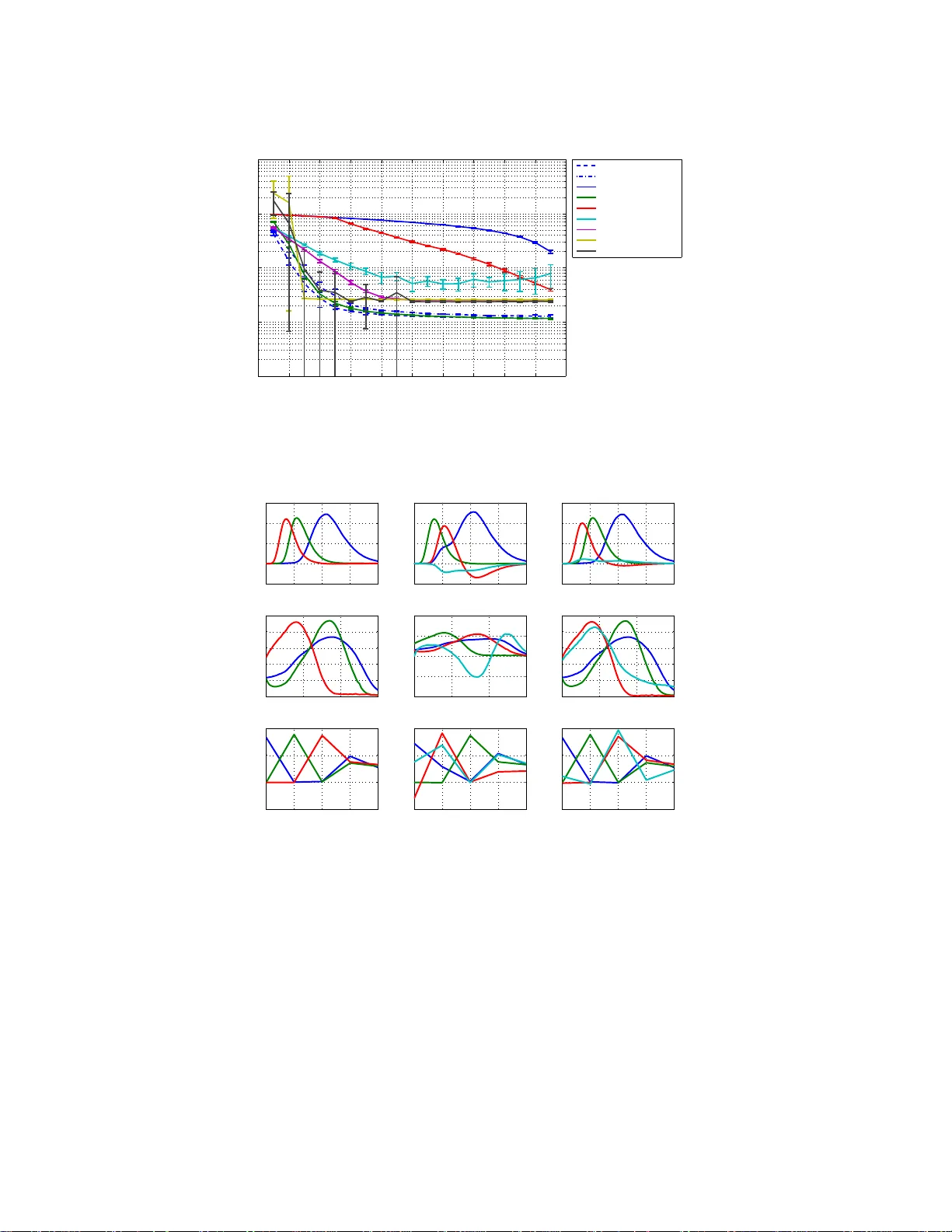
ESTIMA TION OF LO W-RANK TENSORS VIA CONVEX OPTIMIZA TION ∗ R YOT A TOMIOKA † , K OH EI HA Y ASHI ‡ , AND HISASHI KASHIMA † Abstract. In this paper, we propose three approac hes f or the estimation of the T uck er decom- posi tion of m ulti- wa y arra ys (tensors) from partial observ ations. All app roac hes are formulated as con vex minimi zation problems. Therefore, the minimum is gu aran teed to b e unique. The proposed approac hes can automatically estimate the n umber of factors (rank) through the optimization. Thus, there is no need to sp ecify the rank b eforehand. The k ey tec hnique we emplo y is the trace norm regularization, which is a p opular approac h f or the estimation of low-rank matrices. In addition, we prop ose a simple heuristic to impr o v e the interpretab ility of the obtained f actorization. The adv an tages and disadv ant ages of three pr oposed approac hes are demonstrated through numerical experiments on b oth synt hetic and real world datasets. W e show that the pr oposed conv ex opti- mization based approaches are m ore accurate in predictiv e p erformance, faster, and more reli able in reco v ering a known multilinear structure than con v en tional approac hes. 1. In tro duction. Multi-wa y data analy sis ha ve recently become increasingly po pular suppor ted b y modern computational pow er [23, 37]. Originally dev elo pe d in the field of psychometrics and chemometrics, its applica tions can now also b e found in s ignal pro cessing (for exa mple, for indep endent comp onent a nalysis) [14], neuro- science [29], and data mining [28]. Decompos itio n of multi-w ay arrays (or tensors) into small num b er of fa c tors hav e b een o ne of the main co ncerns in multi-w ay data analysis, bec ause interpreting the original multi-w ay data is often imp os sible. There ar e tw o po pular mo dels fo r tenso r decomp os ition, namely the T uc ker decomp os ition [4 4, 1 3] and the CANDECOMP/ P ARAF A C (CP) decomp os ition [11, 19]. In both cases , con- ven tionally the estimation pr o cedures ha ve been formulated as non-conv e x o ptimiza- tion problems, which ar e in g eneral only g ua ranteed to con verge lo cally and could po tent ially suffer fr om p o or lo cal minima. Moreov er, a popula r approach for T uck er decomp osition kno wn as the higher order or thogonal itera tion (HOO I) ma y con verge to a stationary point that is not ev en a lo cal minimizer [15]. Recently , convex formulations for the estimation of low-rank matrix , which is a sp ecial case of tensor, have bee n intensiv ely studied. After the pioneering work of F az e l et al. [16], co n vex optimization has b een used for co llab orative filter ing [38], multi-task learning [3], and classific a tion ov er matr ices [40]. In a dditio n, there a re theoretica l developmen ts that (under some conditions) g uarantee p erfe ct r e c onstruction o f a low- rank matrix from partial measuremen ts via co nv ex estimation [10, 32]. The key idea here is to replace the r ank of a matrix ( a non-conv ex f unction) b y the so-called t race norm (also known as the nuclear norm) o f the matrix. One go a l of this pap er is to extend the tra ce-norm regula r ization for more than t wo dimensions. There have recently b een related w o rk by L iu et al. [27] and Signoretto et a l. [3 6], which co r resp ond to one of the prop ose d approaches in the cur rent pap er. In this paper , we prop ose three formulations fo r the estimation of low rank tensor s . The first approa ch is called “a s a matrix” and estimates the low-rank matrix that is obtained by unfolding (or ma tricizing) the tensor to b e estimated; thu s this approach ∗ This wo rk was supported by MEXT KAKENHI 22700138, 80545583, JST PR ESTO, and NTT Commun ication Science Laboratories. † Departmen t of Mathematical Informatics, The Universit y of T oky o, 7-3-1 Hongo, Bunkyo-ku, T okyo, 113-8656 , Japan ( { tomiok a,kashima } @mist.i.u-tokyo.ac.jp ) ‡ Graduate School of Information Science, Nara Institute of Science and T echnology , 8916-5 T ak a y ama, Ik oma, Nara, 630-0192, Japan ( kohei- h@is.nai st.jp ) , 1 basically treats the unknown tensor a s a ma tr ix and only works if the tenso r is low- rank in the mo de used for the estimation. The second approa ch called “constr aint” extends the first approach by incorp o rating the trace norm p ena lties with resp ect to all mo des simultaneously . Therefore, there is no arbitrar iness in c ho osing a single mo de to work with. How ever, a ll mo des b eing s im ultaneously low-rank mig h t b e a strong assumption. The third a pproach called “mixture” rela xes the as s umption by using a mixture of K tensors , where K is the num b er of mo des of the tensor. Each tensor is regularized t o be low-rank in each mode. W e apply the above three approa ches t o the reconstruction of partially observ ed tensors. In b oth sy nthetic and real-world datas e ts, we show the sup er ior predictive per formance of the propo sed appro aches against co n ven tional expectation maximiza- tion (E M) bas e d estimation of T uck er de c o mpo sition mo del. W e also demons trate the effectiveness of a heur istic to improve the in terpr etability of the core tensor obtained by the prop osed approaches on the amino acid fluo rescence dataset. This pa per is structured a s follows. In the next section, we first review the matrix ra nk and its r e lation to the tra ce norm. Then we review the definition of tensor mo de- k rank, which sugg ests that a low rank tenso r is a low rank matrix when appropria tely unfolded. In Section 3, we prop ose three appr oaches to extend the tr a ce-norm r egulariza tion for the estimatio n of low-rank tenso rs. In Section 4 , we show that the o ptimization problems as so ciated to the propo s ed extensions can be solved efficiently by the alternating direction metho d o f multipliers [17]. In Sec- tion 5, w e show t hrough n umerical exper iment s that one of the prop o sed a pproaches can recover a par tly observed low-rank tensor almos t p e r fectly from sma ller fraction of obs erv ations compared to the co nv entional EM-based T uck er decomp osition algo- rithm. The proposed algorithm shows a sharp thres hold b ehaviour fro m a po o r fit to a nea rly p erfect fit; we n umerically s how tha t the fractio n of samples at the thresh- old is roughly pro po rtional to the sum o f the k -ra nks of the under lying tensor when the tensor dimensio n is fixed. Finally we summarize the pa p e r in Section 6. Earlier version of this manuscript app ea red in NIPS2 010 workshop “T ensors, Kernels, and Machine Lear ning”. 2. Lo w rank matrix and tenso r. In this section, we firs t discuss the connec- tion betw een the r ank of a matrix a nd the trace-nor m regular ization. Then we r eview the CP and the T uck er dec omp osition and the notions o f tens or rank connected to them. 2.1. Rank of a matrix and the trace norm. The rank r of a n R × C matrix X can b e defined as the num ber of nonzero singular v a lues o f X . Here, the singular - v alue decompos itio n (SV D) of X is written as follo ws : X = U dia g ( σ 1 ( X ) , σ 2 ( X ) , . . . , σ r ( X )) V ⊤ , (2.1) where U ∈ R R × r and V ∈ R C × r are o rthogona l matr ices, and σ j ( X ) is the j th largest singular- v alue of X . The matrix X is called low-r ank if the rank r is less than min( R, C ). Unfortunately , the r a nk of a ma trix is a nonconv ex function, and the direct minimization of r ank or solving a rank-constr ained proble m is an NP-hard problem [32]. The trace norm is known to b e the tightest conv ex lower b ound of matrix r ank [32] 2 (see Fig. 2.1) a nd is defined as the linear sum of sing ular v a lues as fo llows: k X k ∗ = r X j =1 σ j ( X ) . Int uitiv ely , the trace norm plays the role of the ℓ 1 -norm in the subset selection pro b- lem [39], for the estimatio n of lo w-r ank matrix 1 . The convexit y of the above function follows from the fact that it is the dual norm o f the spe ctral norm k · k (see [6 , Section A.1.6]). Since it is a norm, the trace norm k · k ∗ is a conv ex function. The non- differentiabilit y o f the trace norm at the or igin promotes many singular v alues o f X to b e zero when used as a re g ularizatio n term. In fact, the following minimization problem has a n a nalytic solution known as the sp ectral soft-thr e sholding o pe r ator (see [8]): argmin X 1 2 k X − Y k 2 F ro + λ k X k ∗ , (2.2) where k · k F ro is the F r o b enius norm, and λ > 0 is a regula rization constant. The sp ectral soft-thresho lding oper a tion can be consider ed as a shrink age oper ation on the singular v alue s and is defined as follows: prox tr λ ( Y ) = U max( S − λ, 0 ) V ⊤ , (2.3) where Y = U S V ⊤ is the SVD of the input ma tr ix Y , and the max o p e ration is taken element-wise. W e can see that the spectral soft-thres holding operatio n truncates the singular-v a lues of the input matrix Y s maller than λ to zer o, thus the r esulting matrix X is usually lo w-rank. See also [42] fo r the deriv a tion. F or the recovery of partially observed low-rank ma trix, some theoretical guaran- tees hav e r ecently b een develop ed. Ca nd` es and Rech t [10] s how ed that in the noiseless case, O ( n 6 / 5 r log( n )) samples are eno ugh to per fectly r ecov er the ma trix under uni- form sampling if the rank r is not too la rge, where n = max( R, C ). 2.2. Rank of a tensor. F or higher or der tensors, there ar e several definitions of rank. Let X ∈ R n 1 × n 2 ×···× n K be a K -w ay tensor. The rank o f a tensor (see [2 4]) is defined as the minimum num b er r of comp onents required for r ank-one decomp osition of a giv en tensor X in analogy to SVD as follows: X = r X j =1 λ j a (1) j ◦ a (2) j ◦ · · · ◦ a ( K ) j , = Λ × 1 A (1) × 2 A (2) · · · × K A ( K ) (2.4) where ◦ denotes the outer pro duct, Λ ∈ R r ×···× r denotes a K -wa y diago nal matrix whose ( j, j, j )th elemen t is λ j , and × k denotes the k -mo de matrix pro duct (see Kolda & Bader [23]); in addition, w e define A ( k ) = [ a ( k ) 1 , . . . , a ( k ) r ]. The ab ov e decomp osition mo del is called CANDECOMP [11] or P ARAF A C [19]. It is worth noticing that finding the ab ov e decomp osition with the minimum r is a hard pr oblem; thus there is no straight forward algorithm for computing the rank for higher-order tensors [24]. 1 Note how ever that the absolute v al ue i s not taken here b ecause singular v alue is defined to b e posi tive. 3 −1.5 −1 −0.5 0 0.5 1 1.5 0 1 2 3 Singular value Penalty |x| 0.01 |x| 0.5 |x| |x| 2 Fig. 2.1 . Penalty funct ions | x | p over one singular value x ar e schematic al ly i l lustr ated for various p . The absolute p enalty function | x | is the tightest c onvex lower b ound o f the r ank ( p → 0 ) in the interval [ − 1 , 1 ] . W e c o nsider instead the mo de - k rank of tenso rs, which is the foundation of the T uck e r decomp osition [44, 13]. The mo de- k rank of X , denoted rank k ( X ), is the dimensionality of the space spa nned by the mode- k fib ers o f X . In other words, the mo de- k r ank of X is the rank of the mo de- k unfolding X ( k ) of X . The mo de- k unfolding X ( k ) is the n k × ¯ n \ k ( ¯ n \ k := Q k ′ 6 = k n k ′ ) matrix o bta ined b y concatenating the mo de- k fiber s of X as co lumn vectors. In MA TLAB this can b e obtained a s follows: X=perm ute(X ,[k:K,1:k-1]); X=X(:,: ); where the order of dimensions other than the first dimension k is not imp ortant as long as w e use a consisten t definition. W e say that a K -wa y tensor X is rank-( r 1 , . . . , r K ) if the mo de- k rank of X is r k ( k = 1 , . . . , K ). Unlik e the rank of the tensor , mode-k rank is clearly computable; the computation o f the mode- k r anks of a tensor boils down to the computation the rank of K matrice s . A rank-( r 1 , . . . , r K ) tensor X ∈ R n 1 ×···× n K can be written as X = G × 1 U 1 × 2 U 2 · · · × K U K , (2.5) where G ∈ R r 1 ×···× r K is called a c or e t ensor , and U k ∈ R n k × r k ( n = 1 , . . . , K ) are left s ingular-vectors from the SVD of the mode- k unfolding of X . The ab ove decomp osition is called the T uc ker decomp osition [44, 23]. The definition of a low-rank tensor (in the sense o f T uc k er deco mp os ition) implies that a lo w-r ank tensor i s a lo w-r ank matrix when unfolded appro priately . In order to see t his, we re c a ll that for the T uc ker model (2.5), the mode- k unfolding of X can b e written as follo ws (see e.g., [23]): X ( k ) = U k G ( k ) ( U k − 1 ⊗ · · · ⊗ U 1 ⊗ U K ⊗ · · · ⊗ U k +1 ) ⊤ . Therefore, if the tensor X is low-rank in the k th mode (i.e., r k < min( n k , ¯ n \ k )), its unfolding is a lo w-rank matrix . Con versely , if X ( k ) is a low-rank matrix (i.e., X ( k ) = U S V ⊤ ), we can set U k = U , G ( k ) = S V ⊤ , and other T uck er factors U k ′ ( k ′ 6 = k ) as identit y matrices, and w e obtain a T uck er decompos ition (2.5). 4 Note that if a given tensor X can b e written in the form o f CP decomp ositio n (2.4 ) with rank r , w e ca n always find a rank-( r, r, . . . , r ) T uc ker decomp osition (2.5 ) b y ortho-nor malizing each factor A ( k ) in Eq ua tion (2.4). Therefor e, the T uc ker decom- po sition is more general than the CP decompo sition. How ever, since the cor e tensor G that co rresp onds to singular -v alues in the ma- trix c a se (see E quation (2.1)) is not diagonal in ge ne r al, it is not s traightforw ard to generalize the trace norm fro m matrices to tensors . 3. Three strat egies to extend the trac e-norm regularization to tensors. In this section, we first consider a given tensor as a matr ix by unfolding it at a given mo de k and propo se to minimize the tr a ce nor m o f the unfolding X ( k ) . Next, we extend this to the minimization of the w eighted sum of the trace norms of the unfold- ings. Finally , relaxing the condition tha t the tensor is joi ntly lo w- rank in ev ery mo de in the s econd approach, we pr o p ose a mixture approa ch. F or so lving the o ptimization problems, we use the alternating direction metho d of mult ipliers (ADMM) [17] (also known as the split Bre g man itera tion [18]). The optimizatio n a lgorithms ar e discussed in Section 4. 3.1. T ensor as a matrix. If we assume that the tensor w e wish to estimate is (at least) low-rank in the k th mo de, we can conv er t the tensor estimation problem int o a matrix estimation pr oblem. E xtending the minimization problem (2.2) to accommo date mis s ing entries we hav e the following o ptimization pr oblem for the reconstructio n of partia lly o bserved tensor: minimize X ∈ R n 1 ×···× n K 1 2 λ k Ω( X ) − y k 2 + k X ( k ) k ∗ , (3.1) where X ( k ) is the mo de- k unfolding of X , y ∈ R M is the vector of obs erv ations, and Ω : R n 1 ×···× n K → R M is a linear op era tor that reshap es the prespec ified elements of the input tensor in to an M dimensional vector; M is the num b er of obser v ations. In E quation (3.1), the regular ization constant λ > 0 is mo ved to the denominator of the loss term fro m the numerator of the regularizatio n ter m in Equation (2.2); this equiv alent reformulation allows us to consider the nois eless cas e ( λ → 0) in the same framework. Note that λ can also b e in ter preted as th e v a riance of the Gaussian observ atio n noise model. Since the estimation pro cedure (3.1) is essentially a n estimation of a low-rank matrix X ( k ) , w e know that in the noiseless c a se O ( ˜ n 6 / 5 k r k log( ˜ n k )) samples are enough to p erfectly recover the unknown true tenso r X ∗ , where r k = rank k ( X ∗ ) and ˜ n k = max( n k , ¯ n \ k ), if the rank r k is not to o high [10]. This ho lds regardles s of whether the unknown tenso r X is low-rank in other mo de s k ′ 6 = k . Ther efore, when we can estimate the mo de- k unfolding of X ∗ per fectly , we c a n also recov er the whole X ∗ per fectly , including the ranks of the mo des we did not use during t he estimation. How ever, the success of the ab ov e pro cedure is conditio ne d on the choice of the mo de to unfold the tensor . If we choose a mo de with a larg e rank, even if there a re other mo des with sma lle r r anks, we ca nnot ho pe to recover the tensor from a small nu m be r of samples. V ario us adv anced metho ds [42, 43, 25, 2 2] for the estimation of low-rank matrices can b e used f or solving the minimization problem (3.1). Here we use ADMM to k e e p the presentation concise; see Section 4 for the details. 3.2. Constrained o ptimization of l o w rank tensors. In order to exploit the rank deficiency of mor e than o ne mo de, it is natural to consider the follo wing 5 extension of the estimation pro cedure (3.1) minimize X ∈ R n 1 ×···× n K 1 2 λ k Ω( X ) − y k 2 + K X k =1 γ k k X ( k ) k ∗ . (3.2) This is a convex optimization problem, beca use it can b e reformulated as follows: minimize x , Z 1 ,..., Z K 1 2 λ k Ω x − y k 2 + K X k =1 γ k k Z k k ∗ , (3.3) sub ject to P k x = z k ( k = 1 , . . . , K ) , (3.4) where x ∈ R N is the v ectorization of X ( N = Q K k =1 n k ), P k is the matrix representa- tion o f mo de- k unfolding (note tha t P k is a per mut ation matr ix ; th us P k ⊤ P k = I N ), Z k ∈ R n k × ¯ n \ k is an auxiliary matrix of the same size as the mo de- k unfolding of X , and z k is the v ectorization of Z k . With a sligh t abus e of notation Ω ∈ R M × N denotes the observ ation opera tor as a matrix. This approach was considered earlier b y Liu et al. [27] and Signo retto et a l. [36]. Liu et al. rela xed the co nstraints (3.4) into p enalty terms, ther efore the factor s o b- tained a s the left singular v ectors of Z k do es not equal the factors of the T uc ker decomp osition o f X . Signoretto et al. hav e discussed the gener al Shatten- { p, q } norms for tensors and the relationship betw een the regulariza tion term in E qua- tion (3.2) with γ k = 1 /K (which corresp onds to Sha tten- { 1 , 1 } no rm) and the function 1 K P K k =1 rank k ( X ). 3.3. Mixture of low-rank tensors. The optimization problem (3.3) p enalize s every mo de o f the tensor X to b e jointly low-rank, which might b e to o s tr ict to b e satisfied in practice. Thus we propo se to predict instead with a mixture of K tens o rs; each mixture comp onent is r egulariz e d by the trace norm to b e low-rank in ea ch mode. More specific a lly , we solve the following min imization problem: minimize Z 1 ,..., Z K 1 2 λ     Ω  X K k =1 P k ⊤ z k  − y     2 + K X k =1 γ k k Z k k ∗ . (3.5) Note that when z k = 1 K P k x for all k = 1 , . . . , K , the pro blem (3.5) reduces to the problem (3.3) with γ ′ k = γ k /K . 3.4. In terpretation. All three propose d approaches inherit the lack of unique- ness of the factors from the conv ent ional T uc ker decomposition [23]. Some heuristics to improv e the interpretability of the core tensor G are prop osed and implemented in the N -wa y to olb ox [2]. How e ver, these approaches are all re stricted to ortho g- onal transformations. Her e we present another simple heuristic, whic h is to a pply P ARAF A C decomp os ition on the cor e tensor G . This approach has the following adv antages o ver applying P ARAF A C directly to the or iginal data. Fir s t, the dimen- sionality of the core tensor ( r 1 , . . . , r K ) is automatica lly obtained from the prop o sed algorithms. Therefore, the ra nge o f the num ber of P ARAF A C comp onents that we need to lo ok for is muc h narr ow er than a pply ing P ARAF AC directly to the o riginal data. Second, the P ARAF AC pro blem do es not need to ta ke care of missing en- tries. In other w o r ds, we can separa te the prediction problem and the in terpr e ta tion problem, whic h are s e parately tackled by the pro po sed algor ithms and P ARAF AC, resp ectively . Finally , empirically the prop osed heuristic s e e ms to b e mor e robust in 6 recov ering the underlying factors co mpa red to applying P ARAF A C dir ectory when the rank is miss p ecified (see Section 5.2). More pr ecisely , let us consider the se cond “Co nstraint” approach. Let U 1 . . . , U K be the left sing ular vectors of the a uxiliary v ar iables Z 1 , . . . , Z K . F r om Equa tion (2.5) we can obtain the core tenso r G as follows: G = X × 1 U 1 ⊤ × 2 U 2 ⊤ · · · × K U K ⊤ . Let A (1) , . . . , A ( K ) be the factors obtained b y the P ARAF A C decomp osition of G a s follows: G = Λ × 1 A (1) × 2 A (2) · · · × K A ( K ) . Therefore, w e have the follo wing deco mpo sition X = Λ × 1 ( U 1 A (1) ) × 2 ( U 2 A (2) ) · · · × K ( U K A ( K ) ) , (3.6) which gives th e k th factor a s U k A ( k ) . 4. Optimization. In this section, we descr ib e the optimization algor ithms ba sed on the alternating directio n metho d o f multipliers (ADMM) for the pro blems (3.1), (3.3), and (3.5). 4.1. ADMM. The a lternating direction metho d o f m ultipliers [17] (see also [5 ]) can b e considered as an approximation of the metho d of m ultipliers [31, 2 1] ( see also [4, 3 0]). The metho d of mult ipliers generates a sequence of primal v ariables ( x t , z t ) and m ultipliers α t by iteratively minimizing the so called aug ment ed Lagr angian (AL) function with r esp ect to the pr imal v a riables ( x t , z t ) and updating the multip lier vector α t . Let us consider the following linear equality constra ined minimizatio n problem: minimize x ∈ R n , z ∈ R m f ( x ) + g ( z ) , (4.1) sub ject to Ax = z , (4.2) where f and g are bo th conv ex functions. The AL function L η ( x , z , α ) o f the above minimization problem is wr itten as follo ws : L η ( x , z , α ) = f ( x ) + g ( z ) + α ⊤ ( Ax − z ) + η 2 k Ax − z k 2 , where α ∈ R m is the Lag rangian multiplier vector. Note that when η = 0, the AL function reduces to the o rdinary Lagra ngian function. Intuitiv ely , the additional pena lty term enforces the equality constr a int to be satisfied. Ho wever, different from the p enalty metho d (whic h was used in [27]), there is no need to increase the penalty parameter η very large, whic h usually mak e s the problem po or ly conditioned. The o riginal metho d o f multipliers p er forms minimization of the AL function with resp ect to x a nd z jointly follow ed by a multiplier update as follows: ( x t +1 , z t +1 ) = a rgmin x ∈ R n , z ∈ R m L η ( x , z , α t ) , (4.3) α t +1 = α t + η ( A x t +1 − z t +1 ) . (4.4) Int uitiv ely s pea king, the mu ltiplier is upda ted prop ortiona lly to the violation of the equality co nstraint (4.2). In this sense, η can also b e regar ded as a s tep-size parameter . 7 Under fairly mild conditions, the abov e metho d co nv erg es sup er-linear ly to a so lution of the minimization problem (4.1); see [34, 41]. How ever, the joint minimization of the AL function (4 .3) is often ha rd (see [4 1] for an exception). The ADMM decouples the minimization with resp ect to x a nd z as follows: x t +1 = argmin x ∈ R n L η ( x , z t , α t ) , (4.5) z t +1 = argmin z ∈ R m L η ( x t +1 , z , α t ) , (4.6) α t +1 = α t + η ( A x t +1 − z t +1 ) . (4.7) Note that the new v alue o f x t +1 obtained in the first line is used in the upda te of z t +1 in the second line. The multiplier upda te step is identical to that of the ordinary method of multipliers (4.4). It can be shown that the abov e algor ithm is an application of firmly nonexpansive mapping a nd that it converges to a solutio n of the original pr oblem (4.1). Surprisingly , this is true for any p ositive p enalty pa rameter η [26]. This is in con trast to the fact that a rela ted appr oach c a lled fo rward-backw ar d splitting [26] ( which was us e d in [3 6]) con verges only when the step-size parameter η is c hos en appropriately . 4.2. Stopping criterio n. As a stopping criterion for terminating the ab ove ADMM algo rithm, we emplo y the relative duality gap criterion; that is, we stop the algorithm whe n the current primal ob jective v alue p ( x , z ) := f ( x ) + g ( z ) and the la rgest dual ob jective v alue ma x t ′ =1 ,...,t d ( ˜ α t ′ ) o btained in the past s atisfies the following equa lity ( p ( x t , z t ) − max t ′ =1 ,...,t d ( ˜ α t ′ )) /p ( x t , z t ) < ǫ. (4.8) Note that the multiplier vector α t computed in Equation (4.7) canno t be directly used in the co mputation of the dual ob jectiv e v a lue, b ecause typically α t violates the dual constraints. See App endix A for the details . The r eason we use the duality gap is that the criterion is inv ariant to the scale of the observed entries y a nd the s iz e of t he problem N . 4.3. ADMM for the “As a Matrix” approac h. W e c o nsider the following constrained reformulation of problem (3.1) minimize x ∈ R N , Z ∈ R n k × ¯ n \ k 1 2 λ k Ω x − y k 2 + k Z k ∗ , sub ject to P k x = z , (4.9) where x ∈ R N is a v ec torization of X , Z ∈ R n k × ¯ n \ k is an auxilia ry v a riable that corres p o nds to the mo de - k unfolding of X , and z ∈ R N is the vectorization o f Z . The AL function of the ab ov e constr ained minimizatio n pr oblem ca n be written as follows: L η ( x , Z , α ) = 1 2 λ k Ω x − y k 2 + k Z k ∗ + η α ⊤ ( P k x − z ) + η 2 k P k x − z k 2 , (4.10) where α ∈ R N is the Lagrangia n multiplier v ector that corres p o nds to the constraint P k x = z . No te that we rescaled the Lagra ngian m ultiplier vector α by the factor η for the sak e of notationa l simplicit y . 8 Starting from a n initial p oint ( x 0 , Z 0 , α 0 ), w e apply the ADMM explained in the previous section to the AL function (4.1 0). All the s teps (4.5)–(4.7 ) can be implemen ted in closed f orms. First, minimization with resp ect to x yields, x t +1 =  Ω ⊤ y + λη P k ⊤ ( z t − α t )  ./ ( 1 Ω + λη 1 N ) , (4.11) where 1 Ω is an N -dimensional v ector that has one for observed ele men ts and zero otherwise; 1 N is an N - dimensional vector filled with o nes; ./ denotes element-wise division. Note that when λ → 0 (no obse r v ational noise), the ab ov e e x pression can be simplified as follows: x t +1 i = ( ( Ω ⊤ y ) i , i ∈ Ω , ( P k ⊤ ( z t − α t )) i , i / ∈ Ω ( i = 1 , . . . , N ) . (4.12) Here the observed entries of x ar e ov erwr itten by the obser ved v alues y and the unob- served entries are filled with the mo de- k tensorization of the current prediction z t − α t . In the genera l cas e (4.11), the predicted v alues also affect the o bserved en trie s . The primal v ariable x t and the auxiliary v aria ble z t bec omes closer and closer as the opti- mization pro ceeds. This means tha t event ually the m ultiplier vector α t takes non-zero v alues only on t he observed entries when λ → 0. Next, the minimization with r esp ect to Z yields, Z t +1 = prox tr 1 /η  P k x t +1 + α t  , where prox tr 1 /η is the sp ectr al so ft-threshold oper ation (2 .3) in which the argument P k x t +1 + α t is considered as a n k × ¯ n \ k matrix. The last step is the mult iplier upda te (4.7), whic h can be written as follows: α t +1 = α t +  P k x t +1 − z t +1  . (4.13 ) Note that the step-size parameter η do es not appear in (4.1 3 ) due to the rescaling of α in (4.10). The sp eed of co n vergence of the algor ithm mildly dep ends o n the choice of the step-size η . Here as a guideline to choose η , we r equire that the algo r ithm is inv ariant to scala r multiplication of the ob jective (4.9). More precisely , when the input y a nd the re g ularizatio n co nstant λ are b oth m ultiplied b y a co nstant c , the s olution of the minimiza tion (4.9) (o r (3.1 )) s ho uld rema in essentially the sa me as the orig ina l problem, except that the solution x is also multiplied b y the constant c . In or der to make the algor ithm (see (4.11 )-(4.13)) follow the same path (except that x t , z t , and α t are a ll multiplied b y c ), we need to scale η inv ersely pr op ortiona l to c . W e can also see this in the A L function (4.10); in fact, t he first t wo terms scale linea rly to c , and also the la st t wo terms sca le linearly if η scales inv ers e ly to c . Therefo r e we c ho o s e η as η = η 0 / std( y ), where η 0 is a constant and std( y ) is the standard deviation of the observed v alues y . 4.4. ADMM for the “Constraint” approac h. The AL function of the con- strained minimization problem (3.3)-(3.4) ca n be written as follo w s : L η ( x , { Z k } K k =1 , { α k } K k =1 ) = 1 2 λ k Ω x − y k 2 + K X k =1 γ k k Z k k ∗ + K X k =1  η α k ⊤ ( P k x − z k ) + η 2 k P k x − z k k 2  . 9 Note that we r escaled the multiplier vector α by the factor η as in the previous subsection. Starting from an initial p oint ( x 0 , { Z 0 k } K k =1 , { α 0 k } K k =1 ), we tak e similar steps as in (4.11)-(4.13) except that the last tw o steps are p e rformed for all k = 1 , . . . , K . That is, x t +1 =  Ω ⊤ y + λη X K k =1 P k ⊤ ( z t k − α t k )  ./ ( 1 Ω + ληK 1 N ) , (4.14) Z t +1 k = prox tr γ k /η  P k x t +1 + α t k  ( k = 1 , . . . , K ) , (4.15 ) α t +1 k = α t k + ( P k x t +1 − z t +1 k ) ( k = 1 , . . . , K ) . (4.16) By c o nsidering the scale inv a riance o f the algorithm, we choose the step-size η as η = η 0 / std( y ) as in the previous subsection. 4.5. ADMM for the “Mixture” approac h. W e co ns ider the following dual problem of the mixture formulation (3.5): minimize α ∈ R M , W k ∈ R n k × ¯ n \ k λ 2 k α k 2 − α ⊤ y + K X k =1 δ γ k ( W k ) , (4.17) sub ject to w k = P k Ω ⊤ α ( k = 1 , . . . , K ) , where α ∈ R M is a dua l vector; W k ∈ R n k × ¯ n \ k is an a uxiliary v aria ble that cor re- sp onds to the mo de- k unfolding of Ω ⊤ α , and w k ∈ R N is the vectorization of W k ; the indicator function δ λ is defined a s δ λ ( W ) = 0, if k W k ≤ λ , and δ λ ( W ) = + ∞ , otherwise, where k · k is the spectral norm (maxim um singula r-v alue o f a matrix). The AL function for the problem (4.1 7) can b e written as follows: L η ( α , { W k } K k =1 , { z k } K k =1 ) = λ 2 k α k 2 − α ⊤ y + K X k =1 δ γ k ( W k ) + K X k =1  z k ⊤ ( P k Ω ⊤ α − w k ) + η 2 k P k Ω ⊤ α − w k k 2  Similar to the prev ious tw o a lgorithms, we star t from an initial point ( α 0 , { W 0 k } K k =1 , { z 0 k } K k =1 ), and compute the following steps: α t +1 = ar gmin α L η ( α , { W t k } K k =1 , { z t k } K k =1 ) W t +1 k = ar gmin W k L η ( α t +1 , { W k } K k =1 , { z t k } K k =1 ) z t +1 k = z t k + η ( P k Ω ⊤ α t +1 − w t +1 k ) . (4.18) The above steps can be computed in closed fo rms. In fact, α t +1 = 1 λ + η K  y − Ω X K k =1 P k ⊤ ( z t k − η w t k )  , (4.19) W t +1 k = pro j γ k ( P k Ω ⊤ α t +1 + z t k /η ) , (4.20) where the pro jection op era to r pro j λ is the pro jectio n onto a ra dius λ -sp ectral-nor m ball, as f ollows: pro j λ ( w ) := U min( S , λ ) V ⊤ , 10 where W = U S V ⊤ is the SVD of the matricization of the input v ector w . Mor eov er , combining the tw o steps (4.20) and (4.18 ), w e hav e (see [41]) z t +1 k = prox tr γ k η  z t k + η P k Ω ⊤ α t +1  . (4.21) Note that we recover the sp ectral soft-threshold op eration prox tr γ k η by co mb ining the t wo steps . Therefor e, we can simply iterate steps (4.19) and (4.21) (note that the term η w t k in (4.19) ca n be computed from (4.18) as η w t k = z t − 1 k + η P k Ω ⊤ α t − z t k .) In o r der to see that the m ultiplier vector z t k obtained in the ab ov e steps conv erges to the pr imal solution of the mixture formulation (3 .5), w e take the deriv ative of the ordinary La grang ian function L 0 with r e s pe ct to α and W k ( k = 1 , . . . , K ) a nd obtain the followin g optimalit y conditions: α = 1 λ  y − Ω X K k =1 P k ⊤ z k  , P k Ω ⊤ α ∈ ∂ γ k k Z k k ∗ ( k = 1 , . . . , K ) , where w e used the r elationship w k = P k Ω ⊤ α , and the fact that ∂ δ γ k ( W k ) ∋ z k implies w k ∈ ∂ γ k k Z k k ∗ bec ause the tw o functions δ γ k and γ k k · k ∗ are conjugate to each other; see [3 3, Cor. 2 3.5.1]. By combining the ab ove t wo equatio ns , we obtain the optimalit y condition for the mixture formulation (3.5 ) as follows: − 1 λ P k Ω ⊤  y − Ω X K k =1 P k ⊤ z k  + ∂ γ k k Z k k ∗ ∋ 0 ( k = 1 , . . . , K ) . As in the previous t wo s ubsections, we require that the alg orithm (4 .18)-(4.21) is inv a riant to scalar m ultiplica tio n of the input y and the r egulariza tion constant λ by the s ame consta n t c . Since z t k app ears in the fina l solution, z t k m ust sca le linea rly with resp ect to c . Th us from (4.18), if α t k and w t k are constants with resp ect to c , the step-size η must scale linearly . In fact, fr o m (4.19) and (4.20), we can see that these t wo dual v a riables rema in constant when y , z t k , and η a r e m ultiplied by c . Therefore, we choose η = std( y ) /η 0 . 5. Numerical exp e riment s. In this section, w e firs t present results on tw o synthetic datasets. Finally we apply the prop osed metho ds to the Amino acid fluo- rescence data published b y Bro and A ndersson [7]. 5.1. Syn thetic exp erim e n ts. W e randomly generated a rank-(7,8,9) tensor of dimensions (50,50,20) b y dr awing the cor e fro m the standard normal distribution and m ultiplying its each mode by an or thonormal factor r a ndomly drawn from the Haa r measure. W e rando mly s elected some elements o f the true tensor for training and kept the re maining elemen ts for tes ting. W e used the algorithms describ ed in the previous section with the tole r ance ǫ = 10 − 3 . W e choo se γ k = 1 for s implicity in the later t wo a pproaches. The step-size η is chosen a s η = η 0 / std( y ) for the first t wo approa ches and η = std( y ) /η 0 for the third appro ach with η 0 = 0 . 1. F o r the first tw o approaches, λ → 0 (zero observ ation er ror) was used; see (4 .1 2). F or the last approach, w e used λ = 0. The T ucker decompo sition algorithm tucker from the N -way toolb ox [2] is also included a s a baseline, for which we used the corre c t rank (“exact”) and the 20% higher r ank ( “large ”). Note that all prop osed approaches ca n find the rank automatically . The generalization error is defined as follows: error = k y pred − y test k k y test k , 11 0 0.1 0.2 0.3 0.4 0.5 0.6 0.7 0.8 0.9 1 10 −4 10 −3 10 −2 10 −1 10 0 Fraction of observed elements Generalization error As a Matrix (mode 1) As a Matrix (mode 2) As a Matrix (mode 3) Constraint Mixture Tucker (large) Tucker (exact) Optimization tolerance Fig. 5.1 . Comp arison of thr e e stra te gies, tensor as a matrix (“As a M atri x ”), c onstr aine d optimization (“Constr aint”), and mixtur e of low-r ank tensors (“Mixtur e”) on a synthetic r ank- (7 , 8 , 9) tensor (t he dim ensions ar e 50 × 50 × 20 ). Also t he T ucker de c omp osition with 20% higher r ank (“lar ge”) and with the c orr e ct r ank (“ex act”) implemente d in t he N -way to olb ox [2] ar e include d as ba selines. The gener alization erro r is plotte d against the fr action of observed elements of the underlying low-r ank tensor. Also the tol er anc e of optimization ( 10 − 3 ) is shown. 0 0.2 0.4 0.6 0.8 1 0 10 20 30 40 50 Fraction of observed elements Computation time (s) As a Matrix Constraint Mixture Tucker (large) Tucker (exact) Fig. 5.2 . Comp arison of c omputation times. where y test is the vectorization of the unobse r ved en tries a nd y pred is the prediction computed by the alg o rithms. F or the “As a Matrix” strategy , er r or for each mo de is re p o rted. All alg orithms were implemented in MA TLAB a nd ran on a co mputer with tw o 3.5GHz Xeon pro cessor s and 32GB of RAM. The exp eriment w a s repea ted 20 times and averaged. Figure 5.1 shows the re sult of tensor c ompletion using three stra tegies we pro - po sed a b ov e, a s well as the T uck er decomp os itio n. A t 35% o bs erv ation, the propo sed “Constraint” obtains nearly p erfect gene r alization. Interestingly ther e is a shar p tra n- sition from a p o or fit (generaliza tio n erro r > 1 ) to an almo st p er fect fit (generaliz a tion error ≃ 1 0 − 3 ). The “ As a Matrix” a pproach also show similar transitio n for mo de 1 and mo de 2 (ar ound 40%), and mo de 3 (around 8 0%), but even the first transition is slow er than the “Co nstraint” appro ach. The “Mixture” a pproach s hows a transition around 70% slightly faster than the mo de 3 in the “As A Matr ix” approach. T ucker shows early decr e ase in the gener alization er ror, but when the rank is misspecified (“large” ), the er ror remains almost constant; even when the correct r ank is k nown 12 0 20 40 60 80 0 0.1 0.2 0.3 0.4 0.5 0.6 0.7 0.8 0.9 1 [10 12 13] [10 12 9] [16 6 8] [17 13 15] [20 20 5] [20 3 2] [30 12 10] [32 3 4] [40 20 6] [40 3 2] [40 9 7] [4 42 3] [5 4 3] [7 8 15] [7 8 9] [8 5 6] Sum of true ranks Fraction required for perfect reconstruction Fig. 5.3 . F r action of observations at the thr eshold plotte d against the sum of true r anks. Numb ers in the bra ckets denote t he k - r ank of the underlying tensor. The dimension of the te nsor i s (50,50,20 ). (“exact”), the con vergence is slo w er th an the propo sed “Constraint ” a pproach. The prop osed con vex approaches a re not only a c curate but also fa st. Fig. 5.2 shows the computation time of the pro p o sed approa ches and EM-ba sed T uck er de- comp osition aga ins t the fra ction of obser ved ent ries. F or the “As a Matr ix” approach the total time for all mo des is plotted. W e can see that t he “As a Matrix” and “Con- straint” approa ches are roughly 4–1 0 times faster than the conv entional EM-base d tuc ker decomp osition. W e ha ve further investigated the condition fo r the threshold behaviour us ing the prop osed “Constra int” appro ach. Her e we genera ted different pro ble ms of different core dimensions ( r 1 , r 2 , r 3 ). The sum of mo de- k ranks is defined as min( r 1 , r 2 r 3 ) + min( r 2 , r 3 r 1 ) + min ( r 3 , r 1 r 2 ). F or eac h proble m, w e apply the “Constraint” a pproach for increasingly large fraction of o bserv ations and determine when the g eneralizatio n error falls b elow 0 . 01 . Fig. 5.3 shows the fraction of o bserv ations req uir ed to obtain generaliza tion e r ror b elow 0 . 01 (in other w o r ds, the fra c tio n at the thre s hold) aga inst the sum of mo de- k ra nks defined a bove. W e can see that the fraction at the threshold is r oughly pr o p ortional to the sum of the mo de- k ra nks of the underlying tensor. W e do not have any theoretical argument to support this o bserv ation. Acar et al [1] also empirically discussed condition f or successful recov e r y for the CP decomposition. Figure 5.4 show another synthetic exp eriment. W e ra ndo mly g e nerated a rank- (50 , 5 0 , 5 ) tenso r of the same dimens io ns as ab ov e . W e chose the same par ameter v alues γ k = 1, λ → 0, ǫ = 10 − 3 , and η 0 = 0 . 1. Here we can see that interestingly the “Constraint” appro ach per fo rm p o orly , wher eas the “mo de 3” and “Mixture ” perfor m clearly b etter than other algorithms. It is na tural that the “mo de 3” appro ach works well because the true tenso r is only lo w-rank in the third mo de. In co nt rast, the “Mixture” appr oach ca n automatica lly detect the rank-deficient mo de, because the regular iz ation t erm in the form ula tion (3.5) is a linear s um of three ( K = 3) penalty terms. The linear s um structure enfor ces spar sity acr o ss Z k . Therefore, in this case Z 1 and Z 2 were switched off, and “Mix ture” approa ch y ielded a lmost identical results to the “ mo de 3” approach. 5.2. Amino acid fluorescence data. The amino acid fluorescence data is a semi-realistic data contributed b y Br o and Andersson [7], in which they measured the fluorescence o f five lab o r atory- made solutions that each contain different a mounts of tyrosine, tryptopha n and phenylalanine. Since the “factors” are known to b e the 13 0 0.2 0.4 0.6 0.8 1 10 −3 10 −2 10 −1 10 0 Fraction of observed elements Generalization error As a Matrix (mode 1) As a Matrix (mode 2) As a Matrix (mode 3) Constraint Mixture Tucker (large) Tucker (exact) Optimization tolerance Fig. 5.4 . Synthetic exp eriment on a r ank- (50 , 50 , 5) tensor of dimensions 50 × 50 × 20 . Se e also Fig. 5.1. three amino acids , this is a perfect da ta for t esting whether the propos e d metho d can automatically find those factors. F or the exp er imen ts in this subsectio n, we chose the same parameter setting γ k = 1, λ → 0, ǫ = 10 − 3 , and η 0 = 0 . 1. Setting λ → 0 corr esp onds to assuming no obser v ational noise. This can b e justified by the fact that the origina l data is already appr oximately low-rank (ra nk-(3 , 3 , 3)) in the sense of T ucker decompo sition. The dimensionality of the o riginal tensor is 201 × 61 × 5, which corresp ond to emis- sion wa velength (25 0–45 0 nm), excitation wa velength (240–3 00 nm), and samples, resp ectively . Fig. 5.5 s how the gener alization err or obtained by the prop osed approaches a s well a s EM-base d T ucker a nd P ARAF A C decomp ositions. Her e P ARAF A C is included bec ause the dataset is orig inally des igned for P ARAF A C. W e can see that the prop osed “Constraint” approach show fast decrease in generalization er ror, which is compar able to the P ARAF AC mo del knowing the cor rect dimensio n. T uc ker decomp osition of rank-(3 , 3 , 3) p e rforms as go o d as P ARAF A C models when mo re than half the en tries are observed. How ever, a slightly lar ger rank-(4 , 4 , 4) T uck er decompo sition could not decrease the error below 0 . 0 5. Fig. 5 .6 show the factors obtained by fitting directly three-comp onent P ARAF A C mo del, four-co mpo nent P ARAF AC mo del, a nd a pplying a four comp onent P ARAF A C mo del to the core o btained by the prop osed “ Co nstraint” a pproach. The fraction of observed entries was 0 . 5. The t wo conv entional approaches used EM iteration for the estimatio n of missing v a lues . F or the prop osed mo del, the dimensio nality of the core was 4 × 4 × 5; this was obtained b y keeping the singular-v a lues of the auxiliar y v ariable Z k that a r e lar ger tha n 1% of its la rgest singula r-v alue for each k = 1 , . . . , K . Then we applied a fo ur -comp onent (fully-obser ved) P ARAF AC mo del to this core a nd obtained the factors as in E quation (3.6 ). Interestingly , a lthough the four comp onent- P ARAF AC mo del is r edundant for this pr oblem [7], the prop osed approach seem to be more robust than applying four- comp onent P ARAF A C directly to the data. W e can see tha t the shape of the ma jor three co mp one nts (blue, g reen, red) o btained b y the prop o s ed approa ch (the rig ht column) are mor e similar to the three-co mp one nt P ARAF AC model (the left column) than t he four-comp onent P ARAF A C model (the center column). 6. Summary . In this pap er we hav e prop osed three strategies to extend the framework of trace no rm re gularizatio n to the es tima tio n of partially o bserved low- rank tensors. The prop o sed approaches a r e form ulated in conv ex optimization prob- 14 0 0.1 0.2 0.3 0.4 0.5 0.6 0.7 0.8 0.9 1 10 −3 10 −2 10 −1 10 0 10 1 Fraction of observed elements Generalization error As a Matrix (mode 1) As a Matrix (mode 2) As a Matrix (mode 3) Constraint Mixture Tucker [4 4 4] Tucker [3 3 3] PARAFAC(3) PARAFAC(4) Fig. 5.5 . Genera lization p erformanc e of pr op ose d met ho ds on the amino acid fluor e sc enc e data is c omp ar e d to c onventional EM-b ase d T ucker de c omp osition and P ARAF AC. Se e also Figur es 5.1 and 5.4. 250 300 350 400 450 −2000 0 2000 4000 6000 Proposed(4) 240 260 280 300 0 0.05 0.1 0.15 0.2 0.25 1 2 3 4 5 −0.5 0 0.5 1 250 300 350 400 450 −2000 0 2000 4000 6000 PARAFAC(4) 240 260 280 300 −0.4 −0.2 0 0.2 0.4 1 2 3 4 5 −0.5 0 0.5 1 250 300 350 400 450 −2000 0 2000 4000 6000 PARAFAC(3) Emission loadings 240 260 280 300 0 0.05 0.1 0.15 0.2 0.25 Excitation loadings 1 2 3 4 5 −0.5 0 0.5 1 Sample loadings Fig. 5.6 . F actors obtaine d by thr ee-c omp onent P ARAF A C (left), four-c omp onent P ARAF AC (c enter), and the heuristic pr op ose d i n Se cti on 3.4 (right) at the fr action of observ ation 0 . 5 . Even when a r e dundant f our-co mp onent P ARAF AC is used in t he p ost- pr o c essing, the pr op ose d heuristic estimates the factors mor e r eliably t han dir e c tly a pplying the P ARAF A C mo del. lems a nd the ra nk of the tensor deco mpo sition is automatically determined through the optimization. In the sim ulated exp eriment, tenso r completion using the “Constraint” a pproach show ed nearly p erfect reco nstruction from only 35% observ ations . The prop osed ap- proach shows a sharp threshold behaviour a nd we hav e empirically found that the fraction of samples at the thres hold is ro ughly prop o rtional to the sum of mo de- k ranks of the under lying tensor. W e hav e als o shown the weakness o f the “Co nstraint” approach. When the un- 15 known tenso r is only lo w-rank in certain mo de, the assumption that the tenso r is low-rank in e very mo de, which under lies the “Cons traint” approach, is to o strong. W e hav e demonstrated that the “ Mixture” approach is more effective in this case. The “Mix ture” appr o ach can automatically detect the rank-defic ie n t mo de a nd lead to better p erformance. In the amino ac id fluorescence datas et, we hav e shown that the prop osed “Co n- straint” a pproach outp erforms conv entional E M-based T uc ker decomp ositio n and is comparable to P ARAF AC mo del with the correct n umber of compo nent s. More over, we have demonstrated a simple heuristic to obtain a P ARAF AC-style decomposition from the deco mp os ition obtained by the prop o sed method. Moreov e r , we hav e shown that the propo sed heuris tic ca n reliably recover the true facto r s even when the num b er of P ARAF AC facto rs is m issp ecified. The prop osed approaches can b e extended in man y w ays. F or exa mple, it w ould be imp orta nt to handle no n- Gaussian no ise mo del [12, 2 0]; for e xample a tensor version of robust PCA [9] would b e highly desirable. F or clas sification over tensors, extension o f the a pproach in [40] would b e mea ningful in applications including bra in- computer int erface; see also [35] for a nother recent appr oach. It is also imp ortant to extend the pro po sed a pproach to handle larg e s c ales tensors that ca nnot b e kept in the RAM. Combination of the first-order optimization prop osed by Aca r et al. [1] with our approach is a promising direction. Moreov er, in order to understa nd the threshold behaviour, further theoretical analysis is necessar y . App endix A. Computation of the dual o b jectiv e s. In this Appe ndix, we show how we co mpute the dua l ob jective v alues for the computation of the relative duality gap (4.8). A.1. Computation of dual ob jective for the “As a Matrix” approac h. The dual pro blem of the cons trained minimiza tio n problem (4 .9) can b e wr itten a s follows: maximize α ∈ R N − λ 2   Ω P k ⊤ α   2 + y ⊤ Ω P k ⊤ α (A.1) sub ject to ¯ Ω P k ⊤ α = 0 , k A k ≤ 1 . (A.2) Here ¯ Ω : R N → R N − M is the linear op erato r that r eshap es the elements of a given N dimensional vector that cor r esp ond to the unobser ved e n tries into an N − M dimensional vector. In addition, A ∈ R n k × ¯ n \ k is the matr ic iz ation o f α and k · k is the spectr a l norm (ma x im um singular v alue ). Note that the multiplier v ector α t obtained through ADMM does no t sa tis fy the ab ov e tw o co nstraints (A.2) . Therefor e, similar to the appr o ach used in [45, 41], we a pply the fo llowing transfor mations. First, we compute the pro jection ˆ α t by pro jecting α t to the equalit y constraint. This ca n b e done easily by s etting the elements o f α t that corres p o nd to unobserved ent ries to zer o . Seco nd, w e compute the maxim um singular v alue σ 1 of the ma tricization of ˆ α t and shrink ˆ α t as follo ws: ˜ α t = min(1 , 1 /σ 1 ) ˆ α t . Clearly this op er a tion do es not vio late with the equa lit y constra int . Finally we sub- stitute ˜ α t int o the dual ob jectiv e (A.1) to compute the relative dualit y gap as in Equation (4.8). 16 A.2. Computation of dual ob jective for the “Constraint” approac h. The dual pro blem of the cons trained minimiza tio n problem (3 .3) can b e wr itten a s follows: maximize { α k } K k =1 − λ 2     Ω K P k =1 P k ⊤ α k     2 + y ⊤ Ω K P k =1 P k ⊤ α k , (A.3) sub ject to ¯ Ω K P k =1 P k ⊤ α k = 0 , k A k k ≤ γ k ( k = 1 , . . . , K ) . Here the anti-observ ation op era to r ¯ Ω is defined as in the la st subse c tio n, and A k ∈ R n k × ¯ n \ k is the ma tricization of α k ( k = 1 , . . . , K ). In order to obtain a dual feasible point from the current multiplier vectors α t k ( k = 1 , . . . , K ), we apply similar transforma tio ns as in the last subse c tio n. Firs t, we compute the pro jection to the equality constr aint. This ca n b e done by computing the sum over α t 1 , . . . , α t K for each unobserved ent ry . Then the sum divided by K is subtracted from eac h corres po nding entry f or k = 1 , . . . , K . Let us denote b y ˆ α t k the m ultiplier vectors after the pro jection. Next, we compute the largest singular- v a lues σ k, 1 = σ 1 ( ˆ A t k ) where ˆ A t k is the matricization o f the pr o jected multiplier vector ˆ α t k for k = 1 , . . . , K . Now in or der to enforc e the inequality constr a ints, we define the shrinkage factor c as follo ws: c = min(1 , γ 1 /σ 1 , 1 , γ 2 /σ 2 , 1 , . . . , γ K /σ K, 1 ) . (A.4) Using the abov e shrink age factor, w e obtain a dual feasible p oint ˜ α t k as follo ws: ˜ α t k = c ˆ α t k ( k = 1 , . . . , K ) . Finally , we s ubstitute ˜ α t k int o the dual ob jectiv e (A.3) to c o mpute the relative duality gap as in Equa tio n (4.8). A.3. Computation of dual ob jective for the “Mixture” approac h. The dual problem of the mixture form ulation is a lready given in E quation (4.17). Making the implicit inequalit y constraints explicit, w e can rewrite this as follows: maximize α ∈ R M − λ 2 k α k 2 + α ⊤ y , sub ject to k P k Ω ⊤ α k ≤ γ k ( k = 1 , . . . , K ) . Note that the norm in the second line should b e in terpreted as the sp ectral norm of the matricizatio n of P k Ω ⊤ α . Although the ADMM pres ent ed in Section 4.5 was designed to s olve this dual formulation, we did not discuss how to ev alua te the dua l ob jective. Again the dual vector α t obtained through the ADMM do es not satisfy the inequalit y constraints. In or de r to obtain a dual feasible p o int, we co mpute the la rgest sing ular-v alues σ k, 1 = σ 1 ( P k Ω ⊤ α ) for k = 1 , . . . , K . F r om the singular-v alues σ k, 1 , w e can compute the shrink age factor c as in Equatio n (A.4) in the previous subs e ction. Finally , a dual feasible p oint can b e obtained as ˜ α = c α , which we use for the computatio n of the relative duality gap (4.8). REFERENCES 17 [1] E. Acar, D.M. Dunla vy, T.G. Kold a, and M. Mørup , Sc alable tensor fact orizations with missing data , tec h. rep ort, arXiv:1005.2197v1 [m ath.NA] , 2010. [2] C. A. Andersson and R. Bro , The N -way to olb ox for MA TLAB , Chemometrics & In telligen t Lab oratory Systems, 52 (2000), pp. 1–4. h ttp://www.models.l ife.ku.dk/source/n wa ytoolb ox/. [3] A. Argyriou, T. Evgeniou, and M. Pontil , Multi-task fe atur e le arning , in Adv ances in Neural Inform ation Pr ocessing Syste ms 19, B. Sc h¨ olkopf, J. Platt, and T. Hoffman, eds., MIT Press, Cam br i dge, MA , 2007, pp. 41–48. [4] D. P. Ber tsekas , Constr aine d Optimization and L agr ange Multiplier Metho ds , Academic Press, 1982. [5] S . Boyd, N. P arikh, E. Chu, B. Pelea to, and J. Eckstein , Distribute d Optimization and Statistic al Le arning via the A lternating Dir e ction Metho d of Multipliers , 2011. Unfinished wo rking draft. [6] S . Boyd and L. V andenbe rghe , Convex Optimization , Cambridge Univ er s ity Pr ess, 2004. [7] R. Bro , P ARAF AC. T utorial and applic ations , Chemometrics and In tell i gen t Lab oratory Sys- tems, 38 (1997), pp. 149–171. [8] J .-F. Cai, E. J. Candes, and Z. S hen , A singular value thr esholding algorithm for matrix c ompletion , tec h. rep ort, arXiv:0810.3286, 2008. [9] E. J . Candes, X. Li, Y. Ma, an d J . Wright , R obust princip al c omp onent analysis? , tec h. repor t, arXiv:0912.3599, 2009. [10] E. J. Candes and B. R echt , Exact matrix c ompletion via c onvex optimization , F oundations of Computational M athematics, 9 (2009), pp. 717–772 . [11] J.D. Carroll and J.J. Chang , Analysis of individual diffe renc es i n multidimensional sc aling via an n-way gener alization of “Eckart-Y oung” de c omp osition , Psyc hometrik a, 35 (1970), pp. 283–319 . [12] E. C. Chi and T. G. Kold a , Making tensor factorizations r obust to non-gaussian noise , tec h. repor t, arXiv: 1010.3043v1, 2010. [13] L. De La thauwer, B. De Moor, and J. V a ndew alle , On the b est r ank-1 and r ank- ( R 1 , R 2 , . . . , R N ) appr oximation of higher-or der tensors , SIAM Journal on Matrix Analysi s and Applications, 21 (2000), pp. 1324– 1342. [14] L. De La thauwer and J. V andew alle , Dimensionality r e duction in higher-or der signal pr o- c essing and r ank-( r 1 , r 2 , . . . , r n ) r e duction in multiline ar algebr a , Li near Algebra and its Applications, 391 (2004), pp. 31–55. [15] L. Eld ´ en and B. Sa v as , A Newton–Gr assmann metho d for c omputing the b est multiline ar r ank- ( r 1 , r 2 , r 3 ) appr oximation of a tensor, , SIAM J. Matrix Anal. Appl., 31 (2009), pp. 248–271. [16] M. F azel, H. Hindi, and S. P. Boyd , A R ank Minimization Heuristic with Applic ation to Minimum Or der System Appr oximation , in Pr oc. of the American Control Conference, 2001. [17] D. Gab a y and B. Mercier , A dual algorithm for the solution of nonline ar variational pr oblems via finite element appr oximation , Comput. Math. Appl., 2 (1976), pp. 17–40. [18] T. Goldst ein and S. Osher , The split Br e gman metho d for L1 r egula rize d pr oblems , SIAM Journal on Imaging Sciences, 2 (2009 ), pp. 323–343. [19] R.A. Ha rshman , F ounda tions of the P ARAF AC pr o c e dur e: Mo dels and c onditions for an “explanatory” multi-mo dal factor analysis , UCLA working papers in phonetics, 16 (1970), pp. 1–84. [20] K. Ha y ashi, T. T a kenouchi, T. Shiba t a, Y. Kamiy a, D. Ka to, K. Kunieda, K. Y am ada, and K. Ikeda , Exp onent i al family tensor factorization for missing-values pr e dicti on and anomaly dete ction , in 2010 IEEE Internationa l Conference on Data Mini ng, 2010, pp. 216– 225. [21] M. R. Hestenes , Multiplier and gr adient met ho ds , J. Optim. Theory Appl., 4 (1969), pp. 303– 320. [22] S. Ji and J. Ye , An ac c ele ra te d gr adient metho d for tr ac e norm m inimization , i n Pr o ceedings of the 26th In ternational Conference on Mac hine Learning (ICML2009), New Y ork, NY, 2009, ACM, pp. 457–464. [23] T. G. Kold a and B. W. Bader , T ensor de c omp ositions and applic ations , SIAM Review, 51 (2009), pp. 455–500. [24] J. B. Kruskal , R ank, de c omp osition, and uniqueness for 3- way and n-way arr ays , in Multiwa y data analysis, R. Coppi and S. Bolasco, eds., Elsevier, North-Holl and, Amsterdam, 19 89, pp. 7–18. [25] Z. Lin, M. Chen, L. Wu, and Y. Ma , The Augmente d L agr ange Multiplier M e tho d for Exact R e co very of Co rrupte d L ow-R ank Matric es , M athematical Programming, (2009). submit- ted. 18 [26] P. L. Lions and B. Mercier , Splitting algorithms for the sum of t wo nonline ar op er ators , SIAM Journal on Numerical Analysis, 16 (1979), pp. 964–979 . [27] J. Liu, P. Musialski, P. Wonka, and J. Ye , T ensor c ompletion for estimating missing values in visual da ta , in Prof. ICCV, 2009. [28] M. Mørup , Applic ations of tensor (multiway arr ay) factorizations and de c omp ositions in data mining , Wiley Inte rdisciplinary Reviews: Data M ining and Kno wledge Discov ery , 1 (2011), pp. 24–40. [29] M. Mørup, L.K. Hansen, C.S. Herrmann, J. P arna s, and S.M. Arnfred , Par al lel factor analysis as an explor atory to ol for wavelet tr ansforme d eve nt-r elate d EEG , NeuroImage, 29 (200 6), pp. 938–947 . [30] J. Noced al and S . Wright , Numeric al Optimization , Springer, 1999. [31] M. J. D. Pow ell , A metho d for nonline ar co nstr aints in minimization pr oblems , in Optimiza- tion, R. Fletcher, ed., Academic Press, London, N ew Y ork, 1969, pp. 283–298. [32] B. Recht, M. F azel, and P.A. P arrilo , Guar ante ed minimum-r ank solutions of linea r matrix e quations via nucle ar no rm minimization , SIAM Review, 52 (2010), pp. 471–50 1. [33] R. T. R ockafellar , Convex Analysis , Pr inceton University Press, 1970. [34] R. T. Rockafellar , Augmente d L agr angians and applic ations of the pr oximal p oint algorithm in c onvex pr o gr amming , Math. of Oper. Res., 1 (197 6), pp. 97–116. [35] M. S ignoretto, L. De La thauwer, and J .A.K. Su ykens , Convex multiline ar esti mation and op er atorial r epr esentations , in NIPS2010 W orkshop: T ensors, Ker nels and Mac hine Learning (TKML), 2010. [36] , Nucle ar norms for tensors and their use for c onvex multiline ar est imation , T ech . Rep ort 10-186, ESA T-SIST A, K.U.Leuve n, 2010. [37] A.K. Smilde, R. Br o, a nd P. Geladi , Multi-way analysis with applic ations in the chemic al scienc es , Wiley , 2004. [38] N. Srebro, J . D. M. Rennie, an d T. S. Jaakkola , Maximum-mar gin matrix factorization , in Adv ances in Neural Information Processing Systems 17, Lawrence K . Saul, Y air W eiss, and L ´ eon Bottou, eds., MIT Press, Cambridge, MA, 2005, pp. 1329–1336. [39] R. Tibshirani , R e gr ession shrinkage and sele ction via the lasso , J. Ro y . Stat. Soc. B, 58 (1996), pp. 267–288 . [40] R. Tomioka and K. Aihara , Classifying matric es with a sp e ctr al r e g ularization , in Pro ceedings of the 24th In ternational Conference on M achine Learning (ICML2007), ACM Press, 2007, pp. 895–902 . [41] R. Tomioka, T. Suzuki, and M. Sugiy am a , Sup er-line ar c onver genc e of dual augmente d- L agr angian algo rithm for sp arsity r e gularize d estimation , tec h. report, 2009. [42] R. Tomioka, T. Suzuki, and M. Su g iy ama , Augmente d La gr angian metho ds for le arning, sele cting, and c ombining fe atur es , i n Optimization for Mac hi ne Learning, Suvrit Sra, Se- bastian No wo zin, and Stephen J. W r i gh t, eds., MIT Press, 2011. [43] R. Tomioka, T. Suzuki, M . Sugiy ama, and H. Kashima , A fast augmente d l agr angian algo - rithm for le arning low-r ank matric es , in Proceedings of the 27 th Annual In ternational Con- ference on Mac hine Learning (ICML2010), Johannes F ¨ urnkranz a nd Thorsten Joac hims, eds., Omnipress, 2010. [44] L. R. Tucker , Some mathematic al notes on thr e e-mo de factor analysis , Psychometrik a, 31 (1966), pp. 279–311. [45] S. J. Wright, R. D. Now a k, and M. A. T. Figueiredo , Sp arse r ec onstruction by sep ar able appr oximation , IEEE T rans. Signal Pro cess., 57 (2009), pp. 2479–2493 . 19