A Simple Data-Adaptive Probabilistic Variant Calling Model

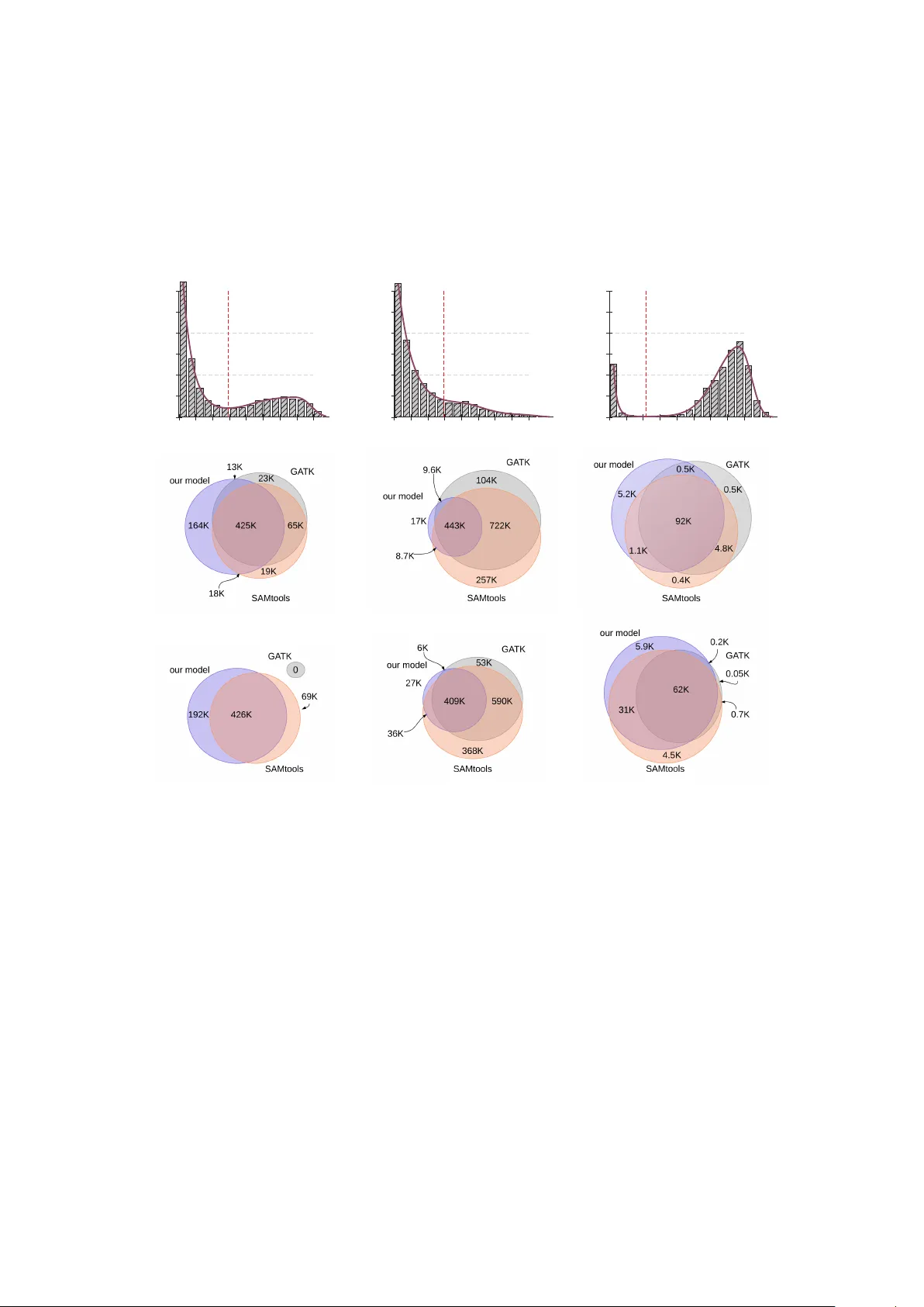
A Simple Data-Adaptive Pr obabilistic V ariant Calling Model Steve Hoffmann 1,2,3 ∗ , Peter F . Stadler 2 − 8 , and Korbinian Strimmer 9,10 19 May 2014; revised 10 January 2015 1 Junior Research Gr oup T ranscriptome Bioinformatics, University Leipzig, Härtelstraße 16-18, Leipzig, Germany 2 Interdisciplinary Center for Bioinformatics and Bioinformatics Group, University Leipzig, Här- telstraße 16-18, Leipzig, Germany 3 LIFE Research Center for Civilization Diseases, University Leipzig, Härtelstraße 16-18, Leipzig, Germany 4 Department of Theoretical Chemistry , University V ienna, Währinger Straße 17, V ienna, Austria 5 RNomics Group, Fraunhofer Institute for Cell Therapy and Immunology – IZI, Perlickstraße 1, Leipzig, Germany 6 Max-Planck-Institute for Mathematics in the Sciences, Inselstraße 22, Leipzig, Germany 7 Center for non-coding RNA in T echnology and Health, University of Copenhagen, Grøn- negårdsvej 3, Fr ederiksberg, Denmark 8 Santa Fe Institute, 1399 Hyde Park Road, Santa Fe, USA 9 Institute for Medical Informatics, Statistics and Epidemiology , University of Leipzig, Härtel- straße 16–18, D-04107 Leipzig, Germany 10 Dept. of Epidemiology and Biostatistics, Imperial College London, Norfolk Place, London W2 1PG, UK. ∗ T o whom corr espondence should be addressed. Email: steve@bioinf.uni-leipzig.de 1 Abstract Background: Several sources of noise obfuscate the identification of single nu- cleotide variation (SNV) in next generation sequencing data. For instance, err ors may be introduced during library construction and sequencing steps. In addition, the reference genome and the algorithms used for the alignment of the reads are further critical factors determining the ef ficacy of variant calling methods. It is crucial to account for these factors in individual sequencing experiments. Results: W e introduce a simple data-adaptive model for variant calling. This model automatically adjusts to specific factors such as alignment errors. T o achieve this, several characteristics are sampled from sites with low mismatch rates, and these are used to estimate empirical log-likelihoods. These likelihoods are then combined to a scor e that typically gives rise to a mixtur e distribution. From these we determine a decision threshold to separate potentially variant sites from the noisy background. Conclusions: In simulations we show that our simple pr oposed model is compet- itive with frequently used much more complex SNV calling algorithms in terms of sensitivity and specificity . It performs specifically well in cases with low allele frequencies. The application to next-generation sequencing data reveals stark differ - ences of the score distributions indicating a strong influence of data specific sources of noise. The proposed model is specifically designed to adjust to these dif ferences. 2 Background Recent studies report a strikingly low concordance of currently available methods and pipelines for identification of single nucleotide variation (SNV), both somatic and germline, indicating that both computational methods as well as sequencing pr otocols have a major impact on the sensitivity and specificity of the variation calling tool (O’Rawe et al., 2013). Specifically , the allelic fraction as well as the coverage of the variant allele are crucial determinants for the statistical benchmarks (Xu et al., 2014; Y u and Sun, 2013). Practical guidelines of SNV callers such as GA TK (McKenna et al., 2010) or SAMtools (Li et al., 2009) suggest to apply rigorous postprocessing filters to reduce the number of false positive calls. Other studies indicate that the application of these filters leads to a substantial impr ovement of the concordance of the callers (Liu et al., 2013). Nevertheless, applying stringent thresholds for variables such as the strand bias, the coverage or read start variation bears the risk of losing important information (Pabinger et al., 2014). These authors emphasize that the differ ent algorithmic and statistical components of a variant caller have to be evaluated as a whole and cannot not be meaningfully judged as single components. If DNA library preparation pr otocols and sequencing machines were able to produce error -free and unbiased sequences of sufficient length the task of variant calling would be easy . Due to various error sources and technical limitations of library preparation, sequencing, and alignment, however , a substantial level of noise complicates the analysis. Since these factors can not be totally controlled during the experiment it seems reasonable to adjust the thresholds for calling a variant depending on the separability of noise and signal, i.e. the true variants. During amplification incorrect nucleotides are incorporated with some error rate e f and during the sequencing step incorrect nucleotides ar e called with the rate e g . After the alignment of the reads to a refer ence sequence we may observe these errors as mismatches or indels. Additional mismatches and indels ar e caused by these refer ence and alignment errors ( e a ). The mismatch rate of a genomic site can be assumed to be the sum δ = e + β , wher e β repr esents the biological variation and e is the compound effect of the technical err ors e f , e g , and e a . Fig. 1 summarizes this situation. The two most commonly used tools for SNV calling methods, SAMtools and GA TK, employ probabilistic models for variant calling. Specifically , the algorithm used by SAMtools (Li, 2011) is based on the likelihood of a genotype which is computed as L ( g ) = 1 m k l ∏ j = 1 [ ( m − g ) ζ j + g ( 1 − ζ j ) ] k ∏ j = l + 1 [ ( m − g ) ( 1 − ζ j ) + g ζ j ] , (1) where g denotes the number of refer ence alleles, m the ploidy , k the number of reads seen at a site, and ζ the error pr obability delivered by the sequencer . Eq. 1 assumes that the first l bases are identical to the r eference, the subsequent bases are not. Subsequently , from this a likelihood for the allele count L ( c ) is obtained. Using the observed allele frequency spectr um φ c as prior information a posterior probability Pr { c } = φ c L ( c ) ∑ c 0 φ c 0 L ( c 0 ) (2) 3 is computed, and a variant is called if Pr { c > 1 } exceeds a certain specified threshold. The GA TK pipeline uses a related probabilistic model for calling variants (DePristo et al., 2011). Similar to SAMtools, the probability Pr { D j | A } of observing the base D j under the hypothesis that A is the true base is calculated by Pr { D j | A } = ( 1 − ζ j D j = A ζ j Pr { A is true | D j is miscalled } otherwise, (3) where Pr { A is true | D j is miscalled } is a pr ecomputed, sequencer specific lookup table. Using prior information based on precomputed heter ozygosity estimations GA TK eval- uates the posterior probabilities of a site to be variant. As with SAMtools calls are determined using fixed preselected thr esholds. Here, we propose a simple probabilistic model for variant calling using a data adaptive threshold on the scale of log-odd-ratios computed from empirical distributions of certain site characteristics. Our appr oach allows to optimally separate simulated SNVs from the noisy background without specification of a threshold for posterior probabilities. In brief, our model starts out by evaluating the mismatch frequencies δ in a data set. Subsequently , we sample several characteristics of the sites with small δ to serve as empirical r eference model. The fundamental idea used her e is that the vast majority of sites is invariant and thus allows to capture the features of the data specific error model. These characteristics ar e then used to form empirical log-likelihoods that are combined to a log-odds type score. T ypically , we observe a mixtur e distribution of two score populations, which we may then separate by a decision thr eshold. Next, we discuss the details of our approach and the pr oposed data-adaptive variant calling algorithm. Subsequently , we apply our method to both synthetic and next generation sequencing data from various species. A refer ence implementation in C99 of our method called haarz is available at http://www.bioinf.uni- leipzig.de/ Software/ . Methods Notation W e denote the position of a site in the refer ence genome by i ∈ [ 1, . . . , n ] where n is the genome length. After aligning the reads to a genome each refer ence base typically has several nucleotides aligned to it. W e refer to the set of all aligned nucleotides as the cross section C i at position i . The coverage at position i is the size | C i | of this set. W e use the index j ∈ [ 1, . . . , | C i | ] to refer to a specific read. The length of read j aligned to site i is denoted by m i j , and the position of a nucleotide in a read is denoted by k i j ∈ { 1, . . . , m i j } . For simplicity , we occasionally leave out the index i when there is no danger of ambiguity . The nucleotide in a cross section can be partitioned into sets of match ( M ) and mismatch ( M ) nuc leotides so that C i = M i ∪ M i . The variant calling algorithm described 4 genome β fragmentation PCR x cycles ǫ f sequencing ǫ g reference alignment ǫ a SNV PCR error sequencing error alignment error Figure 1: Accumulation and sources of errors in next generation sequencing reads. The identification of single nucleotide variations (green dashes) is complicated by various sources of err or . PCR errors accumulate during the amplification and sequencing step. After fragmentation single fragments under go several amplification cycles. Errors are introduced with a rate δ f (red dashes). Further errors are accumulated during sequencing ( δ g ). During the alignment to the r eference further mismatches and indels are introduced ( δ a ). 5 below uses the partition { M i , M i } at each position i to compute an overall score for this particular site. Biological versus technical variation The mismatch rate δ i = | M i | / | C i | is the observed number of mismatches divided by the coverage. The mismatch rate δ i = β i + e i may be decomposed into biological and technical variation, where e i denotes the technical error that accumulated during the preparation, sequencing and alignment steps and β i denotes the biological nucleotide variation at site i . W e aim to distinguish biologically variant positions ( β i > 0) from non-variant positions ( β i = 0), based on the observed mismatch rates δ i and site characteristic scores derived from sequence data or pr oduced during sequencing. Cross sections with high mismatch rates ar e indicative of biological variation in the sample, whereas in cr oss sections with small mismatch rate the mismatches are more likely due to technical err ors. Conversely , in the overwhelming majority of cr oss sections C i we may assume that there is no biological variation pr esent, i.e. β i = 0, and thus mismatches are only caused by technical err ors. For use in the variant calling score we estimate for each δ i the corresponding empiri- cal quantile q ( δ i ) . The motivation for using the quantile rather than the actual value is that it implements a simple normalization of the error . The empirical quantile q ( δ i ) is estimated by tabulating the cumulative fr equencies of δ i across the genome and then reading of f the quantile from the resulting empirical distribution function (ECDF). T o ascertain the probabilities of certain site characteristics, discussed further below , we uniformly sample from sites with 0 < δ i < 0.5. Informally , these characteristics then reflect “backgr ound distributions” of non-variant sites and thus are estimated from sites with less than 50% of mismatches. The degree of biological variation depends on the type of genome. For heterozygous genomes one expects to find predominantly SNP alleles with β i = 0.5 or β i = 1.0, whereas cancer tissues may show mutations with 0 < β i ≤ 1 depending on the het- erogeneity and cancer cell content of the sample. Similarly , arbitrary values of β i will appear in whole population sequencing data. Accordingly , we expect differ ent values of β i for mixtures of sequencing data fr om differ ent individuals. The variant calling algorithm introduced in the following makes no assumptions concerning the presence of diploid genomes, knowledge about the ploidy , homo- or heter ozygosity . Site characteristics In addition to the partitioning of nucleotides at a given site into match and mismatch sets, our algorithm uses the following information, which is typically reported by the sequencer or the read mapper for every site i and read j : • the nucleotide qualities ( Q ), • r elative read position ( P ), 6 • err ors in the alignment ( R ), and • the number of multiple hits ( H ). The nucleotide qualities take on values between 0 and 1 and are given as Q = 1 − ζ , i.e., as probability of a base being corr ect, with values close to 1 corresponding to optimally accurate sequencing. W e dir ectly use Q in computing the variant calling score. The relative r ead position is given by P = k i j / m i j . For the construction of our variant calling score we employ the probability Pr ( M | P ) of a match at a given read position, along with the maximum P M = max P Pr ( M | P ) . The probability of a mismatch is then given by Pr ( M | P ) = 1 − Pr ( M | P ) , and its maximum P M = max P Pr ( M | P ) . W e estimate the probability Pr ( M | P ) empirically , i.e., by appropriately counting matches and mismatches over all sites and reads. The number of errors in the alignment is an integer value gr eater or equal to zer o, and denoted here by R . Finally , the number of multiple hits H describes the number of alignments for each read. The multiplicity of an alignment yields information on the repetitiveness of a genomic r egion. As above for the r elative read position, we tabulate the occurrence of matches for each value of R and and H and correspondingly obtain estimates of the probabilities Pr ( M | R ) and Pr ( M | H ) . Scores for distinguishing variant and non-variant sites Informally , in a non-variant cross section ( β i = 0) we expect that the probability of a match base increases with high nucleotide qualities (good sequencing), low read error rates, few multiple hits and good read positions. Conversely , the probability of mismatching bases in non-variant cross sections incr eases with low nucleotide qualities (poor sequencing), high read error rates, multiple hits and error -prone read positions. For variant sites with β > 0 we expect to have high nucleotide qualities, good read positions and few multiple hits also for the mismatch bases. Consequently , for distinguishing variant from non-variant sites only the mismatching bases ar e relevant. W e introduce four log-odds ratios to formalize and summarize the evidence for a variant over a non-variant based on the above four site characteristics. ∆ Q = 1 | C | ∑ x ∈ M log Q x 1 − Q x for base qualities, ∆ P = 1 | C | ∑ x ∈ M  log Pr ( M | P x ) 1 − Pr ( M | P x ) + log P M P M  for read positions, which ar e rescaled by their r espective maximally attained values P M and P M , ∆ R = 1 | C | ∑ x ∈ M log Pr ( M | R x ) 1 − Pr ( M | R x ) 7 for read err ors, and ∆ H = 1 | C | ∑ x ∈ M log Pr ( M | H x ) 1 − Pr ( M | H x ) for multiple matches. Note that only reads with mismatching bases in a cr oss-section are used for estimation, i.e. match bases ar e ignored. If there ar e only match bases in a cross-section , i.e. if | M | = 0 then the cr oss-section is not consider ed in any component of our model . V ariant calling with adaptive threshold From these log-odds ratios we now construct a total scor e for variant calling by comput- ing, at any position i , S i = ∆ P i + ∆ Q i + ∆ R i + ∆ H i + log q ( δ i ) . This score comprises the four summaries of the site characteristics, as well as the log- quantile of the observed mismatch rate δ i , i.e. the observed number of changes at position normalized by coverage. A low quantile for δ i thus strongly penalizes the overall score. For variant calling we now proceed as follows. W e assume that the majority of the sites ar e non-variant, and only a smaller part is variant, with S i > 0. Thus, the observed distribution of S i will be a mixture distribution, consisting of a null distribution corresponding to the invariant sites and an alternative “contamination” component corresponding to the variant sites. In order to find an optimal adaptive cut-off separating the background from potential variants we estimate the densities by fitting a natural spline using Poisson-regression to the histogram, following the procedur e described by Efron and T ibshirani (1996). Subsequently , we numerically find the location with the minimum density and use it as threshold for separating the two score populations. Specifically , we fit natural splines to the histogram for S i > 0 and numerically determine the local minimum. If there ar e multiple minima the leftmost minimum is used. The corresponding threshold is denoted by S ∗ . In some cases there is no minimum in the histogram of the empirical scores. In this case we use as fall-back solution the upper 95% quantile as threshold. A missing minimum might indicate that the score model does not suf fi ce to r eliably call the variants. Once the threshold S ∗ is established, we declare all sites S i > S ∗ to be variant. In Fig. 2 this pr ocedure is illustrated using data fr om A. thaliana . W e note that by construction of the scor e S i we assume independence of the site characteristics. However , in practice ther e will be correlation, and as alternative one may also consider a fully multivariate construction of the scor e S i . However , this is not without its own drawbacks, as the corr elation among site characteristics may be hard to estimate r eliably . Moreover , as is well known fr om classification and “naive Bayes” analysis, independence models ar e typically rather r obust and often even outperform more complex parameter -rich multivariate models. 8 Score Density 0 2 4 6 8 0.0 0.1 0.2 0.3 0.4 0.5 0.6 Figure 2: Adaptive cutoff determination. The figure shows the distribution of the empirical scores S i > 0 (red continuous line) and the cutoff S ∗ (dotted blue vertical line). The threshold separates potential variants fr om background signal. Results and Discussion Simulation study T o evaluate the reference implementation “ haarz ” of our adaptive model we compared it with the two frequently used SNV callers GA TK (McKenna et al., 2010) and SAMtools (Li et al., 2009). The precise command line settings are summarized in the Appendix. W e simulated next generation sequencing data for the human chromosome 21 using GemSIM (version 1.6) (McElroy et al., 2012) with the default model and coverages ranging from 10, 20, 30, 50, 100, to 200-fold. The simulated content of the variant allele was either 0.2 or 0.5. Simulated r ead length was 100. For mapping we used the aligners that ar e r ecommended for each method. Specifically , we used BW A (Li and Durbin, 2009) to generate the alignments for GA TK and SAMtools. For the refer ence implementation of our model we used segemehl (Hoffmann et al., 2009). After mapping and variant calling we collected for each combination of coverage and variant allele frequencies the number of false positives (FP), true positives (TP), false negatives (FN), and true negatives (TN). From this we computed the r ecall (sensitivity) S E N S = T P / ( T P + F N ) and the positive predictive value P P V = T P / ( F P + T P ) , i.e. the true discovery rate. For the pr oposed data adaptive model we investigated the scor e distribution for all 12 9 experiments (Fig. 3 ). Except for the combination of low coverage (10x) and low variant allele content (20%) we observe the presence of two populations. The separability of these score populations improves with incr easing coverage and variant allele content. In each case, the minimum score for variant calls was automatically set to the value where the density of scores > 0 attains its first first local minimum. Subsequently all positions with a score equal or gr eater were called as SNV and compared to the other callers. All of the tested programs show a good recall and positive predictive value in all 12 simulations. For low allele contents in conjunction with low coverages, however , SAMtools attains comparably low positive predictive values. Surprisingly , after r eaching a maximum recall for the coverage of 100, the recall drops substantially for coverage 200. For the simulations with 50% allele content, all tools show high recalls and good positive predictive values. Again, SAMtools achieves only a comparably low positive predictive value for poorly covered SNVs (Fig. 4 ). Except for the lowest coverage, all tools performed well on these data sets. In Fig. 5 we show results for the challenging case of small minor allele frequencies of 5% and 10%. Our approach compar es well in these rather difficult cases, in contrast to SAMtools and GA TK. For the low coverages, our algorithm does not find a clear cutof f and thus r esorts to the 95% criteria. Since there ar e very few sites with high scores, i.e. S > 0, the recall is low and the positive predictive value is high. As soon as higher coverages are r eached and a minimum is found, the recall is increases substantially . W e note that for low SNP fr equencies in conjunction with low coverages the sample sizes for sampling site characteristics (default sample size: 100000; see Appendix) need to be increased to calculate the distribution of scor es S > 0. Application to data sets The good overlap between the differ ent methods in our simulation study as well as the small number of false positives is in stark contrast to the experience of greatly differing variant calls in r eal life data (e.g. O’Rawe et al., 2013). W e therefor e applied our model to diverse real data fr om both diploid and haploid organisms. Paired end next generation sequencing data for Arabidopsis thaliana (SRR519713), Escherichia coli (ERR163894) and Drosophila melanogaster (SRR1177123) was downloaded under the respective accession numbers from the Short Read Archive ( www.ncbi.nlm. nih.gov/sra ). The Arabidopsis data was aligned to the refer ence genome version 10.5. W ith the data set SRR519713 we obtained a coverage of ∼ 30-fold. The E. coli data set was aligned to the refer ence genome E. coli k12 assembly v1.16. W ith ERR163894 we obtained a coverage of ∼ 60-fold. Finally , SRR1177123 was aligned to the D. melanogaster reference version dm3. The coverage was ∼ 25-fold. For the alignments, calling and filtering we used standard parameters. Precise settings ar e given in the Appendix. The score distributions are shown in first line of Fig. 6 . In the case of the plant A. thaliana and the pr ocaryote E. coli , a clear separation of two populations is observable. On the other hand, the separation of the score populations in D. melanogaster data set is less pronounced. 10 0.0 0.25 0.50 0.75 1.00 -10 -8 -6 -4 -2 0 2 4 6 8 score density 0.0 0.5 1.0 1.5 2.0 0.0 2 4 0.0 0.25 0.50 0.75 1.00 -10 -8 -6 -4 -2 0 2 4 6 8 score density 0.0 0.5 1.0 1.5 2.0 0.0 2 4 6 8 0.0 0.25 0.50 0.75 1.00 -10 -8 -6 -4 -2 0 2 4 6 8 score density 0.0 0.5 1.0 1.5 2.0 0.0 2 4 0.0 0.25 0.50 0.75 1.00 -10 -8 -6 -4 -2 0 2 4 6 8 score density 0.0 0.5 1.0 1.5 2.0 0.0 2 4 6 8 0.0 0.25 0.50 0.75 1.00 -10 -8 -6 -4 -2 0 2 4 6 8 score density 0.0 0.5 1.0 1.5 2.0 0.0 2 4 0.0 0.25 0.50 0.75 1.00 -10 -8 -6 -4 -2 0 2 4 6 8 score density 0.0 0.5 1.0 1.5 2.0 0.0 2 4 6 8 Figure 3: Score distributions of simulated SNV data . The left (right) column shows the score distributions of simulated SNVs with 20% (50%) variant allele content for 20-fold (top), 50-fold (middle) and 100-fold(bottom) coverage. The insets show the density of scores > 0. W ith the incr ease of coverage a population of scores > 0 is clearly distinguishable from the backgr ound. 11 0.0 0.1 0.2 0.3 0.4 0.5 0.6 0.7 0.8 0.9 recall b b b b b b u t u t u t u t u t u t r s r s r s r s r s r s b b b b b b u t u t u t u t u t u t r s r s r s r s r s r s 0.90 0.92 0.94 0.96 0.98 0 20 40 60 80 100 120 140 160 180 200 coverage po sitive predictive value b b b b b b u t u t u t u t u t u t r s r s r s r s r s r s 0 20 40 60 80 100 120 140 160 180 200 coverage b b b b b b u t u t u t u t u t u t r s r s r s r s r s r s b b u t u t r s r s haarz gatk samtools 20% SNP frequency 50% SNP frequency Figure 4: Statistical performance measures on simulated data sets. The data adaptive model implemented in haarz was compared to SAMtools and GA TK in terms of recall and positive predictive value. SNV calling was performed on twelve dif ferent data sets varying in the content of the variant allele (20% and 50%) as well as the simulated coverage (10-200). In all of these scenarios the data adaptive model is at par with both alternative callers. 12 0.0 0.1 0.2 0.3 0.4 0.5 0.6 0.7 0.8 0.9 recall b b b b b b u t u t u t u t u t u t r s r s r s r s r s b b b b b b u t u t u t u t u t u t r s r s r s r s r s r s 0.6 0.7 0.8 0.9 0 20 40 60 80 100 120 140 160 180 200 coverage p ositive p redictive value b b b b b b u t u t u t u t u t u t r s r s r s r s r s 0 20 40 60 80 100 120 140 160 180 200 coverage b b b b b b u t u t u t u t u t u t r s r s r s r s r s r s b b u t u t r s r s haarz gatk samtools 5% SNP frequency 10% SNP frequency Figure 5: Statistical performance measures on simulated data sets with small variant allele frequency . As in Fig. 4 we compare our approach with SAMtools and GA TK with 10% and 5% of minor allele frequencies. 13 In the lower part of Fig. 6 we show the concordance of variant calls of three investi- gated methods for the thr ee data sets. For the well separable cases, the number of calls made by the data adaptive model is equal or higher as compared to the two competing callers. For the D. melanogaster data set our approach is more conservative and reports fewer variants. Most of these, however , are also found by SAMtools and GA TK. About 92% percent of the calls from our model are also supported by both of the other callers and only 4% are not supported by any of the two alternative appr oaches. Fr om the score distributions for D. melanogaster it is clear that there is a large overlap of the two score populations and hence the choice of S ∗ necessarily depends on the desired specificity and/or sensitivity . In the simulated data (Fig. 4 and Fig. 5 ) we see that haarz generally achieve a high recall (sensitivity), and at the same time offers a high positive pr edictive value, (PPV) i.e. low false discovery rate. Thus, for the D. melanogaster data many sites may be ambiguous to call, and our tool will err on the conservative side to maintain a high PPV . Conclusions W e have presented a data adaptive model for variant calling based on easily accessible read characteristics, namely the log-likelihoods of nucleotide qualities, relative r ead positions, alignment errors, multiple hits and the mismatch rate at a position to obtain a score. W ith the exception of nucleotide qualities, which are provided as input by the sequencing method, all log-likelihoods ar e sampled fr om the data itself. W e show that in simulated as well as in real data sets this score gives rise to a mixture distribution that distinguishes between true variants and noise. A spline fit to the overall mar ginal density allows us to determine a decision threshold that optimally separates these score populations. In the simulated data we demonstrated that this simple model is at par with two of the most commonly used pr obabilistic models for SNV calling methods in terms of both sensitivity and specificity . When applying our model to actual next-generation sequencing data, we observe that the distributions of the scores vary significantly among the differ ent data sets. As expected, the clearest separation of the mixture was obtained for the haploid E. coli data set. In addition, the small size of the genome and the absence of r epetitive elements probably improves the separability of the scores. The situation for the two diploid genomes A. thaliana and D. melanogaster is dif ferent. While both genomes have comparable sizes, the separability of the score distributions varies strongly among these two data sets. While a clear minimum can be found for the plant, the mixture in D. melanogaster appears to be more complicated. In this case, by construction our model selects a conservative decision threshold. While the number of calls is similar to the other probabilistic SNV callers in the simulations as well as the next-generations data sets of the plant and the bacteria, it is significantly r educed in the fr uit fly data set. These differ ences indicate that the characteristics of next-generation data sets have a strong impact on the success of variant calling. Furthermor e, we observe that, at least for the score proposed here, a significant dif ference of the separability of the mixtur e distribution can be found 14 Arabidopsis thaliana Drosophila melanogaster Escherichia coli 0 0 . 1 0 . 2 0 . 3 0 . 4 0 . 5 0 1 2 3 4 5 6 7 8 density score 0 0 . 1 0 . 2 0 . 3 0 . 4 0 . 5 0 1 2 3 4 5 6 7 8 density score 0 0 . 1 0 . 2 0 . 3 0 . 4 0 . 5 0 1 2 3 4 5 6 7 8 density score Figure 6: Score distributions and congruence of variant calls in next generation se- quencing data . While a clear separation of score populations is observable for the diploid A. thaliana and the haploid E. coli , only a shallow minimum can be observed in case of D. melanogaster . Hence, in the latter case our model automatically adjusts to the data such that the calling appears to be more conservative: less than 4 percent of the calls are not supported by any caller and 92% of its calls ar e supported both by GA TK and SAMtools. On the other hand, our model calls more variants in the other two cases. 15 between simulated and real data. Thus, we argue that data adaptive components could help to balance the trade-off between sensitivity and specificity . Acknowledgements This r esearch was supported by LIFE (Leipzig Research Center for Civilization Diseases), Leipzig University and the Deutsche Forschungsgemeinschaft under the auspicies of SPP 1590 “Probabilistic Structures in Evolution”, proj. no. ST A 850/14-1. LIFE is funded by the European Union, by the European Regional Development Fund (ERDF), the European Social Fund (ESF) and by the Free State of Saxony within the excellence initiative. W e thank the r eferees for their very helpful comments. 16 References DePristo, M. A., Banks, E., Poplin, R., Garimella, K. V ., Maguir e, J. R., Hartl, C., Philip- pakis, A. A., del Angel, G., Rivas, M. A., Hanna, M., et al. (2011). A framework for variation discovery and genotyping using next-generation dna sequencing data. Nature genetics , 43(5):491–498. Efron, B. and T ibshirani, R. (1996). Using specially designed exponential families for density estimation. Annals Stat. , 24:2431–2461. Hoffmann, S., Otto, C., Kurtz, S., Sharma, C. M., Khaitovich, P ., V ogel, J., Stadler , P . F ., and Hackermüller, J. (2009). Fast mapping of short sequences with mismatches, insertions and deletions using index structur es. PLOS Comp. Biol. , 5:e1000502. Li, H. (2011). A statistical framework for snp calling, mutation discovery , association mapping and population genetical parameter estimation from sequencing data. Bioin- formatics , 27(21):2987–2993. Li, H. and Durbin, R. (2009). Fast and accurate short read alignment with Burrows- Wheeler transform. Bioinformatics , 25:1754–1760. Li, H., Handsaker , B., W ysoker , A., Fennell, T ., Ruan, J., Horner , N., Martin, G., Abecasis, G., Durbin, R., and 1000 Genome Project Data Processing Subgroup (2009). The Sequence Alignment/Map format and SAMtools. Bioinformatics , 25:2078–2079. Liu, X., Han, S., W ang, Z., Gelernter , J., and Y ang, B.-Z. (2013). V ariant Callers for Next-Generation Sequencing Data: A Comparison Study. PLoS ONE , 8(9):e75619+. McElroy, K. E., Luciani, F ., and Thomas, T . (2012). GemSIM: general, error -model based simulator of next-generation sequencing data. BMC Genomics , 13:74. McKenna, A., Hanna, M., Banks, E., Sivachenko, A., Cibulskis, K., Kernytsky , A., Garimella, K., Altshuler , D., Gabriel, S., Daly , M., and DePristo1, M. A. (2010). The Genome Analysis T oolkit: A MapReduce framework for analyzing next-generation DNA sequencing data. Genome Res. , 20:1297–1303. O’Rawe, J., Jiang, T ., Sun, G., W u, Y ., W ang, W ., Hu, J., Bodily , P ., T ian, L., Hakonarson, H., Johnson, W . E., W ei, Z., W ang, K., and L yon, G. (2013). Low concordance of multiple variant-calling pipelines: practical implications for exome and genome sequencing. Genome Medicine , 5(3):28. Pabinger , S., Dander , A., Fischer , M., Snajder , R., Sperk, M., Efremova, M., Krabichler , B., Speicher , M. R., Zschocke, J., and T rajanoski, Z. (2014). A survey of tools for variant analysis of next-generation genome sequencing data. Briefings in Bioinformatics , 15:256–278. 17 Xu, H., DiCarlo, J., Satya, R., Peng, Q., and W ang, Y . (2014). Comparison of somatic mutation calling methods in amplicon and whole exome sequence data. BMC Genomics , 15(1):244. Y u, X. and Sun, S. (2013). Comparing a few snp calling algorithms using low-coverage sequencing data. BMC Bioinformatics , 14(1):274. Appendix Read simulation For the simulation of r eads and allele contents we used the program GemSIM (v . 1.6). W e simulated r eads for the human chromosome 21 (hg19) with dif ferent coverages using an Illumina specific error model (ill100v5_s). python GemReads.py -g simulatedsnps.txt -r chr21.fasta -m ill100v5_s.gzip \ -n -l 100 -q 64 -o Benchmarks and command line parameters For the benchmarks we have aligned the simulated as well as the r eal reads with bwa and called the variants with SAMtools and GA TK. For our own model the reads were aligned using segemehl . The command line parameters and version numbers are given below . a) BW A v 0.6.2 bwa aln > bwa_PE1.sai bwa aln > bwa_PE2.sai bwa sampe bwa_PE1 bwa_PE2 > my.sam b) GA TK v 2.8.1 (GenomeAnalysisTK-2.8-1-g932cd3a) calling: java -jar GenomeAnalysisTK.jar -T UnifiedGenotyper -R \ -I -o filtering: java -jar GenomeAnalysisTK.jar -T VariantFiltration -R -V \ --filterExpression "QD < 2.0 || FS > 60.0 || MQ < 40.0 || HaplotypeScore > 13.0 || \ MQRankSum < -12.5 || ReadPosRankSum < -8.0" --filterName "filter" -o c) SAMtools v 0.1.19 calling: 18 samtools mpileup -uf | bcftools view -bvcg - > bcftools view var.raw.bcf > filtering: varFilter -D100 > d) segemehl v 0.1.7 segemehl.x -d -i -q SRR519713.fastq -D 0 > mysam.sam obtaining site characteristics (written to sorted.haarz.idx): haarz.x -d -q -x -H -Q -M 2000 obtaining site characteristics for low variant allel frequencies: haarz.x -d -q -x -U 0 -X 0 -H -Q -M 2000 calling: haarz.x -d -q -i -M 2000 -F 0.01 -Q -c > haarz.vcf 19