Density Estimation Trees in High Energy Physics

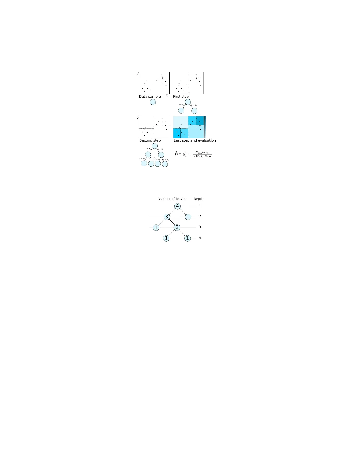
Density Estimation T rees in High Ener gy Physics Lucio Anderlini Istituto Nazionale di Fisica Nucleare – Sesto Fiorentino, Firenze January 30th, 2015 Abstract Density Estimation T rees can play an important role in exploratory data anal- ysis for multi-dimensional, multi-modal data models of large samples. I briefly discuss the algorithm, a self-optimization technique based on kernel density esti- mation, and some applications in High Energy Physics. 1 Intr oduction The usage of nonparametric density estimation techniques has seen a quick gro wth in the latest years both in High Energy Physics (HEP) and in other fields of Science dealing with multi-variate data samples. Indeed, the improv ement in the computing resources av ailable for data analysis allows today to process a much larger number of entries requiring more accurate statistical models. A v oiding parametrization for the distribution with respect to one or more variables allows to enhance accuracy remov- ing unphysical constraints on the shape of the distrib ution. The improv ement becomes more evident when considering the joint probability density function with respect to correlated variables, for whose model a too large number of parameters would be re- quired. Kernel Density Estimation (KDE) is a nonparametric density estimation technique based on the estimator ˆ f KDE ( x ) = 1 N tot N tot X i =1 k ( x − x i ) , (1) where x = ( x (1) , x (2) , ..., x ( d ) ) is the vector of coordinates of the d -variate space S describing the data sample of N tot entries, k is a normalized function referred to as kernel . KDE is widely used in HEP Cranmer (2001); Poluektov (2014) including no- table applications to the Higgs boson mass measurement by the A TLAS Collaboration Aad et al. (2014). The variables considered in the construction of the data-model are the mass of the Higgs boson candidate and the response of a Boosted Decision T ree (BDT) algorithm used to classify the data entries as Signal or Backgr ound candidates Breiman et al. (1984). This solution allo ws to synthesize a set of v ariables, input of the 1 BDT , into a single v ariable, the BDT response, which is modeled. In principle, a multi- variate data-model of the BDT -input v ariables may simplify the analysis and result into a more powerful discrimination of signal and background. Though, the computational cost of traditional nonparametric data-model (histograms, KDE, ...) for the sample used for the training of the BDT , including O (10 6 ) entries, is prohibiti ve. Data modelling, or density estimation, techniques based on decision trees are dis- cussed in the literature of statistics and computer vision communities Ram & Gray (2011); Prov ost & Domingos (2000), and with some optimization they are suitable for HEP as they can contribute to solve both classification and analysis-automation prob- lems in particular in the first, exploratory stages of data analysis. In this paper I briefly describe the Density Estimation T ree (DET) algorithm, in- cluding an innov ati ve and fast cross-validation technique based on KDE and consider few e xamples of successful usage of DETs in HEP . 2 The algorithm A decision tree is an algorithm or a flo wchart composed of internal nodes representing tests of a variable or of a property . Nodes are connected to form branches , each termi- nates into a leaf , associated to a decision . Decision trees are extended to Density (or Probability) Estimation T rees when the decisions are probability density estimations of the underlying probability density function of the tested variables. Formally , the estimator is written as ˆ f ( x ) = N leav es X i =1 1 N tot N (leaf i ) V (leaf i ) I ( x i ) , (2) where N leav es is the total number of leaves of the decision tree, N (leaf i ) the number of entries associated to the i -th leaf, and V (leaf i ) is its v olume. If a generic data entry , defined by the input variables x , would fall within the i -th leaf, then x is said to be in the i -th leaf, and the characteristic function of the i -th leaf, I ( x ) =  1 if x ∈ leaf i 0 if x 6∈ leaf i , (3) equals unity . By construction, all the characteristic functions associated to the other leav es, are null. Namely , x ∈ leaf i ⇒ x 6∈ leaf j ∀ j : j 6 = i. (4) The training of the Density Estimation Tree is divided in three steps: tr ee gr owth , pruning , and cr oss-validation . Once the tree is trained it can be ev aluated using the simple estimator of Equation 3 or some ev olution obtained through smearing or inter- polation . These steps are briefly discussed belo w . 2 2.1 T ree growth As for other decision trees, the tree gro wth is based on the minimization of an estimator of the error . For DETs, the error is the Inte grated Squared Error (ISE), defined as R = ISE( f , ˆ f ) = Z S ( ˆ f ( x ) − f ( x )) 2 d x . (5) It can be shown (see for example Anderlini (2015) for a pedagogical discussion) that, for large samples, the minimization of the ISE is equi valent to the minimization of R simple = − N leav es X i =1  N (leaf i ) N tot  2 1 V (leaf i ) . (6) The tree is therefore grown by defining the replacement error R (leaf i ) = −  N (leaf i )  2 N 2 tot V (leaf i ) , (7) and iterativ ely splitting each leaf ` to two sub-leav es ` L and ` R maximising the residual gain G ( ` ) = R ( ` ) − R ( ` L ) − R ( ` R ) . (8) The growth is arrested, and the splitting a voided, when some stop condition is matched. The most common stop condition is N ( ` L ) < N min or N ( ` R ) < N min ; but it can be OR-ed with some alternativ e requirement, for example on the widths of the leav es. A more complex stop condition is obtained by defining a minimal leaf-width t ( m ) with respect to each dimension m . Splitting by testing x ( m ) is forbidden if the width of one of the resulting leaves is smaller than t ( m ) . When no splitting is allo wed the branch growth is stopped. This stop condition requires to issue the algorithm with a few more input parameters, the leaf-width thresholds, but is very powerful against ov er-training. Besides, the determination of reasonable leaf-widths is an easy task for most problems, once the expected resolution on each v ariable is known. Figure 1 depicts a simple example of the training procedure on a two-dimensional real data-sample. 2.2 T ree pruning DETs can be ov ertrained. Overtraining (or ov erfitting) occurs when the statistical model obtained through the DET describes random noise or fluctuations instead of the underlying distribution. The effect results in trees with isolated leaves with small vol- ume and therefore associated to lar ge density estimations, surrounded by almost-empty leav es. Overtraining can be reduced through pruning , an a posteriori processing of the tree structure. The basic idea is to sort the nodes in terms of the actual improvement they introduce in the statistical description of the data model. Follo wing a procedure common for classification and regression trees, the r e gularized err or is defined as R α (no de i ) = X j ∈ leav es of no de i R (leaf j ) + αC (no de i ) , (9) 3 Data sam ple F irst s tep Second st ep Last step and evalu ation x y x > x 0 x < x 0 x > x 0 x < x 0 y > y 0 y < y 0 x 0 y > y 1 y < y 1 y Figure 1: Simple example of training of a density estimation tree over a two dimen- sional sample. 4 3 2 1 1 1 1 Number of leaves Depth 1 2 3 4 Figure 2: T wo examples of complexity function based on the number of leav es or subtrees, or on the node depth. where α is named r egularization parameter , and the index j runs over the sub-nodes of no de i with no further sub-nodes (its leav es). C (node i ) is the complexity function of leaf i . Sev eral choices for the complexity function are possible. In the literature of clas- sification and regression trees, a common definition is to set C (no de i ) to the number of terminal nodes (or lea ves) attached to node i . Such a comple xity function provides a top-down simplification technique which is complementary to the stop condition. Un- fortunately , in practice, the optimization through the pruning obtained with a number- of-leav es complexity function is ineffecti ve against ov ertraining, if the stop condition is suboptimal. An alternativ e cost function, based on the depth of the node in the tree dev elopment, provides a bottom-up pruning, which can be seen as an a posteriori optimization of the stop condition. An example of the two cost functions discussed is sho wn in Figure 2. If R α (no de i ) > R (no de i ) the splitting of the i -th node is pruned, and its sub- nodes mer ged into a unique leaf. Each node is therefore associated to a threshold value 4 of the regularization parameter , so that if α is lar ger than the threshold α i , then the i -th node is pruned. Namely , α i = 1 C (no de i )   R (no de i ) − X j ∈ leav es of no de i R (leaf j )   . (10) The quality of the estimator Q ( α ) , defined and discussed below , can then be ev al- uated per each threshold value of the regularization parameter . The optimal pruning is obtained for α = α best : Q ( α best ) = max α ∈{ α i } i Q ( α ) . (11) 2.3 Cross-v alidation The determination of the optimal regularization parameter is named cr oss-validation , and many dif ferent techniques are possible, depending on the choice of the quality function. A common cross-validation technique for classification and regression trees is the Leave-One-Out (LOO) cross-validation and consists in the estimation of the underlying probability distribution through a resampling of the original dataset. For each data entry i , a sample containing all the entries but i is used to train a DET . The ISE is redefined as R LOO ( α ) = Z S  ˆ f α ( x )  2 d x − 2 N tot N tot X i =1 ˆ f α not i ( x i ) , (12) where ˆ f α ( x ) is the probability density estimation obtained with a tree pruned with regularization parameter α , and ˆ f α not i ( x ) is the analogous estimator obtained from a dataset obtained removing the i -th entry form the original sample. The quality function is Q ( α ) = − R LOO ( α ) . (13) The application of the LOO cross-validation is very slo w and requires to build one decision tree per entry . When considering the application of DETs to large samples, containing for e xample one million of entries, the construction of a million of decision trees and their e valuation per one million of threshold regularization constants becomes unreasonable. A much faster cross-v alidation is obtained comparing the estimation obtained with the DET with a triangular-k ernel density estimation f k ( x ) = 1 N tot × × N tot X i =1 d Y k =1  1 −     x − x i h k      θ  1 −     x − x i h k      , (14) where θ ( x ) is the Heaviside step function, k runs ov er the d dimensions of the coordi- nate space S , and h k is the kernel bandwidth with respect to the v ariable x ( k ) . 5 The quality function is Q ker ( α ) = − Z S ( f α ( x ) 2 − f k ( x ) 2 ) 2 d x . (15) The choice of a triangular kernel allo ws to analytically solve the inte gral writing that Q ker ( α ) = 1 N 2 tot N leav es X j =1 N (leaf α j ) V (leaf α j ) (2 N j − N (leaf α j )) + const , (16) where leaf α j represents the j -th leaf of the DET pruned with regularization constant α , and N j = N tot X i =1 d X k =1 I j k ( x i ; h k ) = N tot X i =1 d X k =1 " u ( k ) ij − ` ( k ) ij + − ( u ( k ) ij − x ( k ) i ) 2 2 h k sign  u ( k ) ij − x ( k ) i  + + ( ` ( k ) ij − x ( k ) i ) 2 2 h k sign  x ( k ) i − ` k ) ij  # . (17) with sign( x ) = 2 θ ( x ) − 1 , and    u ( k ) ij = min  x ( k ) max (leaf j ) , x ( k ) i + h k  ` ( k ) ij = max  x ( k ) min (leaf j ) , x ( k ) i − h k  . (18) In Equation 18, x ( k ) max (leaf j ) and x ( k ) min (leaf j ) represent the upper and lower boundaries of the j -th leaf, respecti vely . An interesting aspect of this technique is that a lar ge part of the computational cost is hidden in the definition of N j which does not depend on α , and therefore can be calculated only once per node, de facto reducing the computational complexity by a factor N tot × N leav es . 2.4 DET Evaluation: smearing and interpolation One of the major limitations of DETs is the existence of sharp boundaries which are unphysical. Besides, a small variation of the position of a boundary can lead to a lar ge variation in the final result, when using DETs for data modelling. T wo families of solutions are discussed here: smearing and linear interpolation. The former can be seen as a con volution of the density estimator with a resolution function. The effect is that sharp boundaries disappear and residual overtraining is cured, but as long as the resolution function has a fix ed width, the adaptability of the DET algorithms is partially lost: resolution will ne ver be smaller than the smearing function width. An alternative technique is interpolation, assuming some behaviour (usually linear) of the density estimator between the middle points of each leaf. The density estimation 6 at the center of each leaf is assumed to be accurate, therefore o vertraining is not cured, and may lead to catastrophic density estimations. Interpolation is treated here only marginally . It is not very robust, and it is hardly scalable to more than two dimensions. Still, it may represent a useful smoothing tool for samples composed of contributions with resolutions spanning a large interv al, for which adaptability is crucial. 2.4.1 Smearing The smeared version of the density estimator can be written as ˆ f s ( x ) = Z S ˆ f ( z ) w  x − z h k  d x , (19) where w ( x ) is the r esolution function . Using a triangular resolution function w ( t ) = (1 − | t | ) θ (1 − | t | ) , ˆ f s ( x ) = N leav es X j =1 d Y k =1 I j k ( x ; h k ) , (20) where I j k ( x ; h k ) was defined in Equation 17. Note that the ev aluation of the estimator does not require a loop on the entries, factorized within I j k . 2.4.2 Interpolation As mentioned abov e, the discussion of interpolation is restrained to two-dimensional problems. The basic idea of linear interpolation is to associate each x ∈ S to the three leaf centers defining the smallest triangle inscribing x (step named padding or tessellation ). Using the positions of the leaf centers, and the corresponding values of the density estimator as coordinates, it is possible to define a unique plane. The plane can then be “read” associating to each x ∈ S a different density estimation. The key aspect of the algorithm is padding . Padding techniques are discussed for example in de Berg et al. (2008). The algorithm used in the examples belo w is based on Delaunay tessellation as implemented in the ROO T libraries Brun & Rademakers (1997). Exten- sions to more than two dimensions are possible, but non trivial and computationally expensi ve. Instead of triangles, one should consider hyper -volumes defined by ( d + 1) leaf centers, where d is the number of dimensions. Moving to parabolic interpolation is also reasonable, but the tessellation problem for ( d + 2) volumes is less treated in the literature, requiring further dev elopment. 3 T iming and computational cost The discussion of the performance of the algorithm is based on an a single-core C++ implementation. Many-core tree growth, with each core growing an independent branch, is an embarrassing parallel problem. Parallelization of the cross-validation is also pos- sible, if each core tests the Quality function for a different value of the regularization 7 Number of entries 2 10 3 10 4 10 5 10 6 10 CPU Time (s) 2 − 10 1 − 10 1 10 2 10 3 10 4 10 5 10 6 10 Training 40000) × Reading ( KDE Number of entries 2 10 3 10 4 10 5 10 6 10 CPU Time (s) 2 − 10 1 − 10 1 10 2 10 3 10 4 10 5 10 6 10 Training 40000) × Reading ( KDE Figure 3: CPU time to train and evaluate a self-optimized decision tree as a function of the number of entries N tot . On the top, a stop criterion including a reasonable leaf- width threshold is used; on the bottom it is replaced with a very loose threshold. The time needed to train a Kernel Density Estimation (KDE) is also reported for compari- son. parameter α . R OO T libraries are used to handle the input-output, but the algorithm is independent, relying on STL containers for data structures. The advantage of DET algorithms o ver kernel-based density estimators is the speed of training and ev aluation. The complexity of the algorithm is N leav es × N tot . In common use cases, the two quantities are not independent, because for larger samples it is reasonable to adopt a finer binning in particular in the tails. Therefore, depending on the stop condition the computational cost scales with the size of the data sample as N tot to N 2 tot . K ernel density estimation in the R OO T implementation is found to scale as N 2 tot . Reading time scales roughly as N leav es . Figure 3 reports the comparison of the CPU time needed to train, optimize and sample on a 200 × 200 grid a DET ; the time to train a kernel density estimation on the same sample is also reported. The two plots show the results obtained with reasonable and loose stop conditions based on the minimal leaf width. It is interesting to observe that when using a loose leaf-width condition, N leav es ∝ N tot and the algorithm scales as N 2 tot . Increasing the size of the sample, the leaf-width condition becomes relev ant and the computational cost of the DET deflects from N 2 tot , and starts being con venient with respect to KDE. 4 A pplications in HEP In this section I discuss a few possible use cases of density estimation trees in High Energy Physics. In general, the technique is applicable to all problems in volving data modeling, including efficienc y determination and background subtraction. Howe ver , for these applications KDE is usually preferable, and only in case of too lar ge samples, in some de velopment phase of the analysis code, it may be reasonable to adopt DET instead. Here I consider applications where the nature of the estimator, providing fast training and fast integration, introduces multiv ariate density estimation into problems traditionally treated alternatively . The examples are based on a dataset of real data collected during the pp collision programme of the Lar ge Hadron Collider at CERN by the LHCb e xperiment. The dataset has been released by the LHCb Collaboration in the 8 ] 2 c combination [GeV/ π Mass of the K 1.82 1.84 1.86 1.88 1.9 Candidates 0 500 1000 1500 2000 2500 3000 3500 4000 Data sample Model Signal Background Figure 4: In variant mass of the combinations of a kaon and a pion loosely consistent with a D 0 decay . T wo contributions are described in the model: a peaking contribution for signal, where the D 0 candidates are consistent with the mass of the D 0 meson (Signal), and a non-peaking contribution due to random combinations of a kaon and a pion not produced in a D 0 decay (Background). framew ork of the LHCb Masterclass programme. The detail of the reconstruction and selection, not relev ant to the discussion of the DET algorithm, are discussed in Ref. LHCb Collaboration (2014). The data sample contains combinations of a pion ( π ) and a kaon ( K ), two light mesons, loosely consistent with the decay of a D 0 meson. Figure 4 sho ws the in variant mass of the K π combination, i.e . the mass of an hypo- thetical mother particle decayed to the reconstructed kaon and pion. T wo contributions are evident: a peak due to real D 0 decays, with the in variant mass which is consistent with the mass of the D 0 meson, and a flat contribution due to the random combination of kaons and pions, with an in variant mass which is a random number . The peaked contribution is named “Signal”, the flat one is the “Background”. An important aspect of data analysis in HEP consists in the disentanglement of dif- ferent contributions to allo w statistical studies of the signal without pollution from background. In next two Sections, I consider two dif ferent approaches to signal- background separation. First, an application of DETs to the optimization of the rect- angular selection is discussed. Then, a more po werful statistical approach based on likelihood analysis is described. 4.1 Selection optimization When trying to select a relativ ely pure sample of signal candidates, rejecting back- ground, it is important to define an optimal selection strategy based on the variables associated to each candidate. For e xample, a large momentum of the D 0 candidate ( D 0 p T ) is more common for signal than for background candidates, therefore D 0 can- didates with a p T below a certain threshold can be safely rejected. The same strategy can be applied to the transverse momentum of the kaon and of the pion separately , which are obviously correlated with the momentum of their mother candidate, the D 0 meson. Another useful variable is some measure of the consistency of the reconstructed flight direction of the D 0 candidate with its expected origin (the pp vertex). Random combinations of a pion and a kaon are likely to produce D 0 candidates poorly aligned 9 with the point where D 0 are expected to be produced. In the following I will use the Impact Parameter (IP) defined as the distance between the reconstructed flight direction of the D 0 meson and the pp verte x. The choice of the thresholds used to reject background to enhance signal purity often relies on simulated samples of signal candidates, and on data regions which are expected to be well dominated by background candidates. In the example dis- cussed here, the background sample is obtained selecting the D 0 candidates with a mass 1 . 815 < m ( D 0 ) < 1 . 840 GeV/ c 2 or 1 . 890 < m ( D 0 ) < 1 . 915 GeV/ c 2 . The usual technique to optimize the selection is to count the number of simulated signal candidates N S and background candidates N B surviving a giv en combination of thresholds t , and picking the combination which maximizes some metric M , for example M ( t ) = S ( t ) S ( t ) + B ( t ) + 1 =  S N S ( t )  S N S ( t ) +  B N B ( t ) + 1 (21) where  S (  B ) is the normalization factors between the number of entries N ∞ S ( N ∞ B ) in the pure sample and the expected yields S ∞ ( B ∞ ) in the mixed sample prior the selection. When the number of thresholds to be optimized is large, the optimization may require many iterations. Only in absence of correlation between the variables used in the selection, the optimization can be f actorized reducing the number of iterations. For large samples, counting the surviving candidates at each iteration may become very expensi ve. T wo DET estimators ˆ f S ( x ) and ˆ f B ( x ) for the pure samples can be used to reduce the computational cost of the optimization from N tot to N leav es , integrating the distri- bution leaf by leaf instead of counting the entries. The integral of the density estimator in the rectangular selection R can be formally written as Z R ˆ f ( x )d x = 1 N tot N leav es X i =1 V (leaf i ∩ R ) V (leaf i ) N (leaf i ) . (22) The optimization requires to find R = R opt : M I ( R opt ) = max R ⊂S M I ( R ) , (23) with M I ( R ) = S ∞ R R ˆ f S ( x )d x 1 + S ∞ R R ˆ f S ( x )d x + B ∞ R R ˆ f B ( x )d x . (24) Figure 5 reports a projection of ˆ f S and ˆ f B onto the plane defined by the impact parameter (IP) and the proper decay time of the D 0 meson. The two variables are ob- viously correlated, because D 0 candidates poorly consistent with their e xpected origin are associated to a larger decay time in the reconstruction procedure, which is based on the measurements of the D 0 flight distance and of its momentum. The estimation reproduces correctly the correlation, allowing better background rejection combining the discriminating power of the tw o v ariables when defining the selection criterion. 10 Proper Decay Time [ps] 0 D 2 4 6 8 10 Impact Parameter [mm] 0 D 0 0.2 0.4 0.6 0.8 1 1.2 1.4 1.6 1.8 2 Proper Decay Time [ps] 0 D 2 4 6 8 10 Impact Parameter [mm] 0 D 0 0.2 0.4 0.6 0.8 1 1.2 1.4 1.6 1.8 2 Figure 5: Density Estimation of pure signal (top) and pure background (bottom) sam- ples, projected onto the plane of the impact parameter and proper decay time. The entries of the data sample are shown as black dots superposed to the color scale repre- senting the density estimation. 4.2 Likelihood analyses Instead of an optimization of the rectangular selection it is reasonable to separate sig- nal and background using multiv ariate techniques as Classification T rees or Neural Network. A multiv ariate statistic based on likelihood can be built using DETs: ∆ log L ( x ) = log ˆ f S ( x ) ˆ f B ( x ) . (25) The advantage of using density estimators over Classification T rees is that likeli- hood functions from dif ferent samples can be easily combined. Consider the sample of K π combinations described above. Among the v ariables defined to describe each can- didate there are Particle Identification (PID) v ariables, response of an Artificial Neural Network (ANN) trained on simulation, designed to provide discrimination, for exam- ple, between kaons and pions. The distributions of PID variables are very difficult to simulate properly because the conditions of the detectors used for PID are not perfectly stable during the data acquisition. It is therefore preferred to use pure samples of real kaons and pions to study the distributions instead of simulating them. The distribu- tions obtained depends on the particle momentum p , and on the angle θ between the particle momentum and the proton beams. These variables are obviously correlated to the transverse momentum which, as discussed in the previous section, is a powerful discriminating variable, whose distribution has to be taken from simulation, and is in general different from simulated samples. T o shorten the equations, below I apply the technique to the kaon only , but the same could be done for the identification of the pion. The multi variate statistic can therefore be re written as ∆ log L  p T ( D 0 ) , IP , p T ( K ) , p T ( π ) , p K , θ K , PID K K  = = ˆ f S ( p T ( D 0 ) , IP , p T ( K ) , p T ( π )) ˆ f B ( p T ( D 0 ) , IP , p T ( K ) , p T ( K ) , PID K K ) × × ˆ f K (PID K K , p K , θ K ) R d(PID K K ) ˆ f K (PID K K , p K , θ K ) , (26) 11 where PID K K is the response of the PID ANN for the kaon candidate and the kaon hypothesis, and ˆ f K is the DET model built from a pure calibration sample of kaons. The opportunity of operating this disentanglement is due to the properties of the probability distribution functions which are not trivially transferable to Classification T rees. Note that, as opposed to the previous use case, where integration discourages smearing because Equation 22 is not applicable to the smeared version of the density estimator , likelihood analyses can benefit of smearing techniques for the ev aluation of the first term in Equation 26, while for the second term, smearing can be avoided thanks to the large statistics usually a vailable for calibration samples. 5 Conclusion Density Estimation T rees are fast and robust algorithm providing probability density estimators based on decision trees. They can be grown cheaply beyond overtraining, and then pruned through a kernel-based cross-validation. The procedure is computa- tionally cheaper than pure kernel density estimation because the ev aluation of the latter is performed only once per leaf. Integration and projections of the density estimator are also fast, providing an effi- cient tool for many-v ariable problems inv olving large samples. Smoothing techniques discussed here include smearing and linear interpolation. The former is useful to fight overtraining, but challenges the adaptability of the DET algorithms. Linear interpolation requires tessellation algorithms which are no wadays av ailable for problems with three or less variables, only . A few applications to high energy physics hav e been illustrated using the D 0 → K − π + decay mode, made public by the LHCb Collaboration in the framew ork of the Masterclass programme. Selection optimization and likelihood analyses can benefit of different features of the Density Estimation Tree algorithms. Optimization problems require fast inte gration of a many-v ariable density estimator , made possible by its sim- ple structure with leav es associated to constant values. Likelihood analyses benefit of the speed of the method which allo ws to model large calibration samples in a time much reduced with respect to KDE, and offering an accuracy of the statistical model much better than histograms. In conclusion, Density Estimation T rees are interesting algorithms which can play an important role in exploratory data analysis in the field of High Energy Physics, filling a gap between the simple histograms and the expensi ve Kernel Density Estimation, and becoming more and more relev ant in the age of the Big Data samples. Refer ences Aad, Geor ges et al. Measurement of the Higgs boson mass from the H → γ γ and H → Z Z ∗ → 4 ` channels with the A TLAS detector using 25 fb − 1 of pp collision data. Phys.Rev . , D90:052004, 2014. doi: 10.1103/PhysRe vD.90.052004. 12 Anderlini, L. Measur ement of the B + c meson lifetime using B + c → J /ψ µ + ν X decays with the LHCb detector at CERN . PhD thesis, Uni versit ` a degli Studi di Firenze, 2015. Appendix A. Breiman, Leo, Friedman, J. H., Olshen, R. A., and Stone, C. J. Classification and Re- gr ession T r ees . Statistics/Probability Series. W adsworth Publishing Company , Bel- mont, California, U.S.A., 1984. Brun, Rene and Rademakers, Fons. R OOT – an object oriented data analysis framew ork. Nuclear Instruments and Methods in Physics Resear ch Section A: Accelerators, Spectrometer s, Detectors and Associated Equipment , 389(12):81 – 86, 1997. ISSN 0168-9002. doi: http://dx.doi.org/10.1016/S0168- 9002(97) 00048- X. URL http://www.sciencedirect.com/science/article/ pii/S016890029700048X . New Computing T echniques in Physics Research V . Cranmer , Kyle S. Kernel estimation in high-energy physics. Comput.Phys.Commun. , 136:198–207, 2001. doi: 10.1016/S0010- 4655(00)00243- 5. de Berg, Mark, Cheong, Otfried, v an Krev eld, Marc, and Overmars, Mark. Compu- tational Geometry: Algorithms and Applications . Springer-V erlag, 2008. ISBN 978-3-540-77973-5. LHCb Collaboration. LHCb@InternationalMasterclass website. http://goo.gl/NpkyzS, 2014. Poluektov , Anton. Kernel density estimation of a multidimensional efficiency profile. 2014. Prov ost, Foster and Domingos, Pedro. W ell-trained pets: Improving probability esti- mation trees. 2000. Ram, Parikshit and Gray , Alexander G. Density estimation trees. In Pr oceedings of the 17th ACM SIGKDD international conference on Knowledge discovery and data mining , pp. 627–635. A CM, 2011. 13