Cheaper and Better: Selecting Good Workers for Crowdsourcing

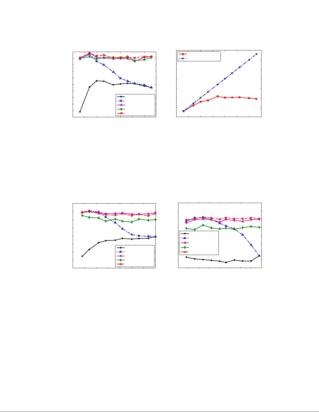
Cheaper and Better: Selecting Good W orkers f or Cr owdsour cing Hongwei Li Department of Statistics Univ eristy of California, Berkeley hwli@stat.berkeley.edu Qiang Liu Department of Computer Science Univ eristy of California, Irvine qliu1@uci.edu Abstract Crowdsourcing provides a popular paradigm for data collection at scale. W e study the problem of selecting subsets of workers from a giv en worker pool to maximize the accuracy under a budget constraint. One natural question is whether we should hire as many workers as the budget allows, or restrict on a small number of top- quality workers. By theoretically analyzing the error rate of a typical setting in crowdsourcing, we frame the worker selection problem into a combinatorial op- timization problem and propose an algorithm to solve it efficiently . Empirical results on both simulated and real-world datasets show that our algorithm is able to select a small number of high-quality workers, and performs as good as, some- times ev en better than, the much larger crowds as the b udget allows. 1 Introduction The recent rise of the crowdsourcing approach has made it possible to collect large amounts of human-labeled data and solv e challenging problems that require human interv ention at a large scale and at a relatively low cost. In micro-task marketplaces such as Amazon Mechanical T urk, the requestors can hire large numbers of online crowd workers to complete human intelligence tasks (HITs) in a short time and with payment as low as several cents per task. Unfortunately , because of the lo w pay and inexperience of the workers, their labeling qualities are often much lo wer than those of experts. A common solution is to add redundancy , asking many crowd workers to answer the same questions, and aggregating their answers; the combined results of the cro wds are often much better than that of an individual worker , sometimes even as good as that of the experts – a phenomenon known as wisdom of cr owds . Howe ver , because the cro wd workers often hav e dif ferent reliabilities due to their diverse back- grounds, it is important to weight their answers properly when aggregating their answers. A large body of work has been proposed to deal with the uncertainty and di versity on the w orkers’ reliabili- ties; these methods often have a form of weighted majority voting where the answers of the majority of the workers are selected, with a weighting scheme that accounts the importance of the different workers according to their reliabilities. The workers’ reliabilities can be estimated either using gold standard questions with kno wn answers (e.g., V on Ahn et al. , 2008 , Liu et al. , 2013 ), or by statisti- cal methods such as Expectation-Maximization (EM) (see, e.g., Dawid and Skene , 1979 , Whitehill et al. , 2009 , Karger et al. , 2011 , Liu et al. , 2012 , Zhou et al. , 2012 ). Our work is motiv ated by a natural question: do more crowd workers necessarily yield better ag- gregated results than less workers? The idea of wisdom of cr owds seems to suggest a confirmati ve answer , since “ larg er cr owds should be wiser ”. From a Bayesian perspectiv e, this would be true if we had perfect knowledge about the workers’ prediction model, and we were able to use an oracle aggregation procedure that performs exact Bayesian inference. Howe ver , in practice, because the workers’ prediction model and reliabilities are ne ver known perfectly , we run the risk of adding 1 noisy information as we increase the number of workers. In the extreme, there may exist a large number of “spammers”, who submit completely random answers rather than good-faith attempts to label; adding these spammers would certatinly deteriorate the results, unless we are able to identify them perfectly , and assign them with zero-weights in the label aggregation algorithm. Even if there exist no extreme spammers, the median-lev el workers may still decrease the o verall accuracy if the y dominate over the small number of high-quality workers. In fact, a recent empirical study ( Mannes et al. , 2013 ) shows that the aggreg ated results of a small number of (3 to 6) high-quality workers are often more accurate than those of much larger cro wds. In this work, we study this phenomenon by formulating a worker selection problem under a budget constraint. Assume we have a pool of workers whose reliabilities hav e been tested by a small number of gold standard questions; under certain label aggregation algorithm, we want to select a subset of workers that maximizes the accuracy , with a budget constraint that the number of workers assigned per task is no more than K . A na ¨ ıve and commonly used procedure is to simply select the top K workers that ha ve the highest reliabilities. Howe ver , due to the noisy nature of the label aggregation algorithms (e.g., majority voting or EM), selecting all the K workers does not necessarily giv e the best accuracy , and may cause a waste of the resource. W e study this problem under a simple label aggregation algorithm based on weighted majority voting, and propose a worker selection method that is able to select fe wer ( ≤ K ) top-ranked workers, while achie ve almost the same, or e ven better aggregated solutions than the na ¨ ıve method that uses more (all the top K ) workers. Our method is deriv ed by framing the problem into a combinatorial optimization that minimizes an upper bound of the error rate, and deriving a globally optimal algorithm that selects a group of top-ranked work ers that optimize the upper bound of the error rate. W e demonstrate the efficienc y of our algorithm by comprehensiv e experiments on a number of real-world datasets. Related work. There are many literatures on estimating the workers’ reliabilities and eliminating the spammers based on a predefined threshold (see e.g., Raykar and Y u , 2012 , Joglekar et al. , 2013 ). Our work instead focuses on selecting a minimum number of highest-ranked workers while dis- carding the others (which are not necessarily spammers). Note that our method has the adv antage of requiring no pre-specified threshold parameters. Our work also should be distinguished with another line of research on online assignment for crowdsouring ( Chen et al. , 2013 , Ho et al. , 2013 , etc.), which hav e dif ferent objectiv es and purposes from our work. Outline. The rest of the paper is organized as follows. W e introduce the background and the problem setting in Section 2 . W e then formulate the work er selection problem into a combinatorial optimiza- tion problem and derive our algorithm in Section 3 . The numerical experiments are presented in Section 4 . W e giv e further discussions in Section 5 and conclude the paper in Section 6 . 2 Background and pr oblem setting Assume there are M cro wd workers and N items (or questions) each with labels from L classes. For notation con venience, we denote the set of w orkers by Ω = [ M ] , the set of items by [ N ] and the set of label classes by [ L ] , where we use [ M ] to denote the set of first M integers. W e assume each item j is associated with an unkno wn true label y j ∈ [ L ] , j ∈ [ N ] . W e also assume that we hav e n contr ol (or gold standard ) questions whose true labels y 0 j ∈ [ L ] , j ∈ [ n ] are known. When item j is assigned to work er i for labeling, we get a possibly inaccuracy answer from the worker , which we denote by Z ij ∈ [ L ] . The workers often ha ve dif ferent expertise and attitude, and hence hav e different reliabilities. W e assume i -th worker labels the items correctly with probability w i , that is, w i = P ( Z ij = y j ) . In addition, assume we ha ve an estimation of the workers’ reliability ˆ w i , which can be estimated either based on the workers’ performance on the control items, or by probabilistic inference algorithms like expectation-maximization (EM). W ith a kno wn reliability estimation ˆ w i , most label aggreg ation algorithms, including the na ¨ ıve majority voting and EM, can be written into a form of weighted majority voting, ˆ y j = argmax k ∈ [ L ] X i ∈ S f ( ˆ w i ) · I ( Z ij = k ) , (1) where f ( ˆ w i ) is a monotonic weighting function that decides how much the answers of worker i contribute to the voting according to the reliability ˆ w i , and I ( · ) is the indicate function. For majority 2 voting, we have f mv ( ˆ w i ) = 1 , which ignores the div ersity of the workers and may performance badly in practice. In contrast, a log-odds weighting function f log ( ˆ w i ) = logit( ˆ w i ) − logit(1 /L ) , where logit( ˆ w i ) def = log( ˆ w i 1 − ˆ w i ) , can be deriv ed using Bayesian rule under a simple model that assumes uniform error across classes; here 1 /L is the probability of random guessing among L classes. Ho wev er, in practice, the log-odds may be over confident (growing to infinite) when ˆ w i is close to 1 or 0. A linearized version f linear ( ˆ w i ) = ˆ w i − 1 /L has better stability , and is simpler for theoretical analysis ( Li et al. , 2013 ). Note that both of f log and f linear hav e properties that are desirable for general weighting functions: Both are monotonic increasing functions of ˆ w i , and take zero value if ˆ w i = 1 /L (to exclude the labels from random guessers); they are both positiv e if ˆ w i > 1 /L (better than random guessers), and are both negati ve if ˆ w i < 1 /L (worse than random guessers). These common properties make f linear and f log work similarly in practice. But since f linear is more stable and simpler for theoretical analysis, we will focus on the linear weighted function f linear for our further dev elopment on the worker selection problem, that is, the labels are aggre gated via (referred as WMV -linear ), ˆ y j = argmax k ∈ [ L ] X i ∈ S ( L ˆ w i − 1) · I ( Z ij = k ) . (2) In the next section, we study the w orker selection problem and propose an ef ficient algorithm based on the analysis of the WMV -linear aggreg ation method. 3 W orker selection by combinatorial optimization The p roblem of selecting an optimal set of workers requires predicting the error rate with a gi ven worker set, which is unfortunately intractable in general. Howe ver , it is con venient to obtain an upper bound of the error rate for the linear weighted majority voting. Theorem 1. Given a set S of worker s, using the weighted majority voting in ( 2 ) with linear weights f linear and an unbiased estimator of the r eliabilities { ˆ w i } i ∈ S that satisfies E [ ˆ w i ] = w i . If the workers’ labels ar e generated independently accor ding the following pr obability P ( Z ij = l | y j = k ) = ( w i if l = k , 1 − w i L − 1 if l 6 = k . (3) Then we have 1 N N X j =1 P ( ˆ y j 6 = y j ) ≤ exp " − 2 F ( S ) 2 L 2 ( L − 1) 2 + ln( L − 1) # , (4) wher e F ( S ) = 1 p | S | X i ∈ S ( Lw i − 1) 2 . (5) Remark: (i) Note that the above upper bound depends on the worker set S and their reliabil- ities w i only through the term F ( S ) . In fact, according to the proof in the supplementary , the term F ( S ) corresponds to the expected gap between the voting score of the true label y i (i.e. P i ∈ S f linear ( ˆ w i ) I ( Z ij = y i ) ) and that of the wrong labels, and hence reflects the confidence of the weighted majority voting. Therefore, F ( S ) represents a score function for the worker set S : if F ( S ) is lar ge, the weighted majority voting is more likely to gi ve correct prediction. (ii) The assumption ( 3 ) used in Theorem 1 implies a “one-coin” model on the workers labels, where the labels are correct with probability w i , and otherwise make mistakes uniformly among the re- maining classes. This is a common assumption to make, especially in theoretical works (see e.g., Karger et al. ( 2011 ), Ghosh et al. ( 2011 ), Joglekar et al. ( 2013 )). It is possible to relax ( 3 ) to a more general “two-coin” model with arbitrary probability P ( Z ij = l | y j = k ) , which, howe ver , may lead more complex upper bounds. In our empirical study on various real-world datasets, we find that F ( S ) remains to be an efficient score function for worker section e ven when the one-coin assumption does not seem to hold. Based on ( 5 ), it is natural to select the workers by maximizing the term F ( S ) , that is, argmax S ⊆ Ω F ( S ) , s.t. | S | ≤ K, (6) 3 Unfortunately , F ( S ) depends on the workers’ true reliabilities w i , which is often unknown. W e instead estimate F ( S ) based on ˆ w i . The following theorem provides an unbiased estimator . Lemma 2. Assume ˆ w i is an unbiased estimator of w i that satisfies E [ ˆ w i ] = w i , and ˆ v ar( ˆ w i ) is an unbiased estimator of the variance of ˆ w i . Consider ˆ F ( S ) = 1 p | S | X i ∈ S G ( ˆ w i ) , (7) wher e G ( ˆ w i ) = ( L ˆ w i − 1) 2 − L 2 ˆ v ar( ˆ w i ) , (8) then ˆ F ( S ) is an unbiased estimate of F ( S ) . Remark: (i) The first term ( L ˆ w i − 1) 2 in ( 8 ) shows that the workers with ˆ w i close to either 1 or 0 should be encouraged; these workers tend to answer the questions either all correctly or all wrongly , and hence are “strongly informati ve” in terms of the predicting the true labels. Note that these work ers with ˆ w i = 0 are strongly informative in that they eliminate one possible value (their answer) for the true labels. On the other side, more work ers also means more noise, so there is a term p | S | for balancing the signal-noise ratio — to encourage hiring “strong” workers instead of only hiring more workers. (ii) A simpler estimation of F ( S ) is to directly plug ˆ w i as w i into ( 5 ), that is, ˆ F plug ( S ) = 1 p | S | X i ∈ S ( L ˆ w i − 1) 2 . (9) Howe ver , this obviously leads to a biased estimator of F ( S ) because of the missing of the v ariance term in ( 8 ). The existence of the variance term is of critical importance: The workers with large uncertainty on the reliabilities should be less fa vorable compared with these with a more confident estimation. Since Lemma 2 does not specify ˆ w i and ˆ v ar( ˆ w i ) , the next theorem provides a concrete example of ˆ F ( S ) , based on which a symmetric confidence interval of F ( S ) can be constructed. Theorem 3. Assume a gr oup of workers ar e tested with n contr ol questions, and let c i be the number of corr ect answers given by worker i on the n contr ol questions. Then an unbiased estimator ˆ w i , with an unbiased estimator of var( ˆ w i ) can be obtained by ˆ w i = c i n and ˆ v ar( ˆ w i ) = c i ( n − c i ) n 2 ( n − 1) . (10) W ith such ˆ w i and ˆ v ar( ˆ w i ) , the corresponding ˆ F ( S ) in ( 7 ) is unbiased and the interval [ ˆ F ( S ) − n ( L − 1) 2 n − 1 α, ˆ F ( S ) + n ( L − 1) 2 n − 1 α ] co vers F ( S ) with pr obability at least 1 − 2 e − 2 α 2 for any α > 0 . Remark: A discussion about the advantage of the unbiasness of ˆ F ( S ) and the symmetric confidence interval is deferred to Section 5 . Based on the estimation of F ( S ) in Theorem 3 , the optimization problem is re written into argmax S ⊆ Ω ˆ F ( S ) , s.t. | S | ≤ K , (11) where ˆ F ( S ) is defined in ( 7 ). Although this combinatorial problem is neither sub-modular nor super- modular , we show it can be e xactly solv ed with a linearithmic time algorithm shown in Algorithm 1 . Algorithm 1 progresses by ranking the workers according to G ( ˆ w i ) in a decreasing order, and se- quentially e valuates the groups of the top-ranked workers, and then finds the smallest group that has the maximal score ˆ F ( S ) . The time complexity of Algorithm 1 is O ( | Ω | log | Ω | ) and the space complexity is O ( | Ω | ) , where Ω is the whole set of w orkers. The following theorem sho ws that Algorithm 1 achiev es the global optimality of ( 11 ). Theorem 4. F or any fixed { ˆ w i } i ∈ Ω . The set S ? given by Algorithm 1 is a global optimum of Pr oblem ( 11 ) , that is, we have ˆ F ( S ? ) ≥ ˆ F ( S ) for ∀ S ∈ Ω that satisfies | S | ≤ K . 4 Algorithm 1 W orker selection algorithm 1: Input: W orker pool Ω = { 1 , 2 , . . . , M } and estimated reliabilities { ˆ w i } i ∈ Ω from n control questions; Number of label classes L ; Cardinality constraint: no more than K work ers per item. 2: x i ← G ( ˆ w i ) , ∀ i ∈ Ω as in ( 8 ), and sort { x i } i ∈ Ω in descending order so that x σ (1) ≥ x σ (2) ≥ . . . ≥ x σ ( M ) , where σ is a permutation of { 1 , 2 , · · · , M } . 3: B ← min( K, M ) , g 1 ← x σ (1) and F 1 ← g 1 . 4: f or k from 2 to B do 5: g k ← g k − 1 + x σ ( k ) and F k ← g k √ k . 6: end f or 7: k ∗ ← min  argmax 1 ≤ k ≤ B F k  . 8: Output: The selected subset of workers S ? ← { σ (1) , σ (2) , · · · , σ ( k ∗ ) } . Remark: As a generalization, consider the follo wing multiple-objecti ve optimization problem, argmax S ⊆ Ω ( ˆ F ( S ) , − | S | ) , s.t. | S | ≤ K, which simultaneously maximizes the score ˆ F ( S ) and minimizes the number | S | of workers actually deployed. W e can show that S ? is in fact a Pareto optimal solution in the sense that there exist no other feasible S that improves ov er ˆ F ( S ) in terms of both ˆ F ( S ) and | S | (details in supplementary). 4 Experimental results W e demonstrate our algorithm using empirical experiments based on both simulated and real-world datasets. The empirical results confirm our intuition: Selecting a small number of top-ranked work- ers may perform as good as, or ev en better than using all the av ailable workers. In particular, we show that our work er selection algorithm significantly outperforms the nai ve procedure that uses all the top K workers. W e find that our algorithm tends to select a very small number of workers (less than 10 in all our experiments), which is very close to the optimal number of the top-rank ed w orkers in practice. T o be specific, we consider the following practical scenario in the experiments: (i) Assume there is a worker pool Ω where each worker has completed a “qualify e xam” with n control questions, which is required by either the platform or a particular task owner . (ii) The task o wner selects a subset of workers from Ω using a work er selection algorithm such as Algorithm 1 based on their performance on the qualify exam. (iii) The selected workers are distributed to answer the N questions of the main interest. (i v) Label aggreg ation algorithms such as WMV -linear or EM are applied to predict the final labels of these N items. Even though our worker selection algorithm is derived when using WMV -linear , we can still use other label aggregation algorithms such as EM, once the worker set is selected. This gives the follow- ing possible combinations of the algorithms that we test: WMV -linear on the top K workers ( WMV top K ), WMV -linear on the work er set S ? selected by Algorithm 1 ( WMV-lin selected ), and WMV with log ratio weights on the selected worker set S ? ( WMV-log selected ), the EM al- gorithm on randomly selected K workers (referred as EM random K ), EM on the top K workers ranked ( EM top K ) and EM on the worker set S ? selected ( EM selected ). W e also implement the work er selection algorithm based on the plugin estimator in ( 9 ) (which is the same as Algorithm 1 , except replacing G ( ˆ w i ) with ( L ˆ w i − 1) 2 ), followed with a WMV -linear aggregation algorithm (referred as WMV-lin plugin ). Since the majority voting tends to perform much worse all the other algorithms, we omit it in the plots for clarity . In each trial of the algorithms on both the simulated and real-world datasets, 10 items are randomly picked from the collected data as the control items, and the workers’ reliabilities { ˆ w i } i ∈ Ω are es- timated based on the accuracy on the control items as ( 10 ). In each trial, the number of workers selected by Algorithm 1 was stored and the a verage number of w orkers w as computed for each b ud- 5 get K . W e terminate all the iterativ e algorithms at a maximum of 100 iterations. All results are av eraged ov er 100 random trials. 4.1 Simulated data 0 5 10 15 20 25 30 35 0.88 0.9 0.92 0.94 0.96 0.98 1 K: max #workers allowed per item Accuracy WMV−lin top K WMV−lin plugin WMV−lin selected 0 5 10 15 20 25 30 35 0 5 10 15 20 25 30 35 K: max #workers allowed per item Avg #workers selected WMV−lin top K WMV−lin plugin WMV−lin selected (a) (b) Figure 1: Performance of different worker selection methods on simulated data. WMV -linear aggre- gation is used in all the cases. W e simulated 31 workers and 1000 items with binary labels, and use 10 control questions. The w orkers’ reliabilities are drawn independently from B eta (2 . 3 , 2) . (a) The accuracies when the budget K varies. (b) The actual number of workers used by dif ferent worker selection methods when K increases. W e generate the simulated data by drawing 31 workers with reliability w i from B eta (2 . 3 , 2) , and we randomly generated 1000 items with true labels uniformly distributed on {± 1 } . The budget K varies from 3 to 31. Figure 1 (a) shows the accuracy of WMV -linear with different worker selection strategies as the budget K changes. W e can see that WMV-lin selected dominates the other methods. Figure 1 (b) sho ws the actual number of workers selected by work er selection algorithm (Algorithm 1 ). WMV -linear based on our selected workers uses a relati vely small number of (al ways < 10 ) workers (the red curve in Figure 1 (b)), and achiev e ev en better performance than WMV-lin top K that uses the entire av ailable budge (the blue line in Figure 1 (b)). W e find that the worker selection algorithm based on the plugin estimator ˆ F plug ( S ) tends to select slightly more work ers, b ut achiev es slightly worse performance than Algorithm 1 based on the bias-corrected estimator ˆ F ( S ) (see WMV-lin select vs. WMV-lin plugin in Figure 1 (a)). This implies the importance of the variance term in ( 8 ), which penalizes the w orkers with noisy reliability estimation. The number of control questions n controls the variance of the reliability estimation ˆ w i , and hence influences the results of the worker selection algorithms. Figure 2 (a) sho ws the results when we v ary n from 3 to 45, with the budget fixed at K = 20 . W e see that the performance of all the algorithms increases when n increases, because we know more accurate information about the workers’ true reliabilities, and can mak e better decision on both choosing the top K workers and selecting workers by Algorithm 1 . In addition, when n increases, the v ariance of ˆ w i decreases and the difference between WMV-linear selected and WMV-linear plugin decreases. Figure 2 (b) shows the results when when we vary the prior parameter a where w i ∼ B eta ( a, 2) , fixed K = 20 and n = 10 . Lar ger a means the workers are more likely to have high reliabilities (i.e., close to 1). W e see from Figure 2 (b) that WMV-lin top K increases as a increases, due to the ov erall improvement of the reliabilities of the top K workers. The performances of WMV-lin selected and WMV-lin plugin improves only slightly , probably because they only select sev eral top workers which is not heavily af fected by a . 6 0 5 10 15 20 25 30 35 40 45 0.8 0.82 0.84 0.86 0.88 0.9 0.92 0.94 0.96 0.98 1 n: number of control items Accuracy WMV−lin top K WMV−lin plugin WMV−lin selected 2.2 2.4 2.6 2.8 3 3.2 3.4 3.6 3.8 4 0.96 0.965 0.97 0.975 0.98 0.985 0.99 0.995 1 a: worker reliability prior Beta(a, 2) Accuracy WMV−lin top K WMV−lin plugin WMV−lin selected (a) (b) Figure 2: Performance of different worker selection methods, (a) when changing the number of control questions n , and (b) when changing the parameter a in the reliability prior B eta ( a, 2) . The budget K is fixed at 20. W e use the WMV -linear aggregation method in all the cases. 4.2 Real data W e test the different worker selection methods on three real-world datasets: two collected by our- selves from the crowdsourcing platform Clickworkers 1 , and one by W elinder et al. ( 2010 ) from Amazon Mechanical T urk. Cr owd-test dataset: In this dataset, 31 workers are asked to answer 75 knowledge-based questions from allthetests.com, which cov er topics such as science, math, common knowledge, sports, geog- raphy , U.S. history and politics and India. All these questions hav e 4 options, and we know the all the ground truth beforehand. W e required each w orker to finish all the questions. A typical e xample of the knowledge-test question is as follo ws: (Question): In what year was the Internet created? (Options): A. 1951; B. 1969; C. 1985; D. 1993. Figure 3 (a) shows the performance of the different methods as the budget K changes. Since EM is widely used in practice, we include the results when using it as the label aggregation algorithm after the workers are selected. W e find that the performance of EM Top K first increases when K is small and then decreases when K is large enough ( ≥ 10 in this case). Our work er selection algorithm selects much smaller number of workers, while much better performance, compared to the top K and random selection methods. Disambiguity dataset: The task here is to identify which W ikipedia page (within 4 possible options) a given highlighted entity in a sentence actually refers to. W e collected 50 such questions in the technology domain with ground truth av ailable, and hire 35 workers through Clickworkers, each of which is required to complete all the questions. A typical example is as follows: (Question): “The Micr osoft .Net F ramework 4 r edistributable pac kage install the .NET F rame work runtime and associated files that ar e r equired to run and develop applications to targ et the .NET F ramework 4”. Which W iki page does “runtime” r efer to? (Options): A. http://en.wikipedia.or g/wiki/Run-time system B. http://en.wikipedia.or g/wiki/Runtime library C. http://en.wikipedia.or g/wiki/Run time (pr ogram lifecycle phase) D. http://en.wikipedia.or g/wiki/Run T ime Infrastructur e (simulation) 1 http://www .clickworker .com/en 7 0 5 10 15 20 25 30 35 0.54 0.56 0.58 0.6 0.62 0.64 0.66 0.68 0.7 0.72 0.74 K: max #workers allowed per item Accuracy EM random K EM top K EM selected WMV−log selected WMV−lin selected 0 5 10 15 20 25 30 35 0 5 10 15 20 25 30 35 K: max #workers allowed per item Avg #workers used Alg. selected workers Alg. random/top K (a) (b) Figure 3: Cro wd-test data. 10 items were randomly selected as control. (a) Performance curve of algorithms with K increasing. (b) Number of work ers the algorithms actually used for each K . Bluebir d dataset: It is collected by W elinder et al. ( 2010 ) and is publicly av ailable. In this dataset, 39 work ers are asked if a presented image contains Indigo Bunting or Blue GroBeak. There are 108 images in total. 0 5 10 15 20 25 30 35 0.5 0.55 0.6 0.65 0.7 0.75 0.8 0.85 0.9 K: max #workers allowed per item Accuracy EM random K EM top K EM selected WMV−log selected WMV−lin selected 0 5 10 15 20 25 30 35 40 0.55 0.6 0.65 0.7 0.75 0.8 0.85 0.9 0.95 K: max #workers allowed per item Accuracy EM random K EM top K EM selected WMV−log selected WMV−lin selected (a) (b) Figure 4: More performance comparison on real-world datasets. (a) The disambiguity dataset: 35 workers and 50 questions in total. (b) The bluebird dataset: 39 workers and 108 questions in total. The settings are the same as that of Figure 3 (a). The number of worker actually used (similar to Figure 3 (b)) are plotted in supplementary . Figure 4 (a) and (b) show the performance of the different algorithms on the bluebird and the dis- ambiguation dataset, respectiv ely . The results are similar to the one in Figure 3 (a). For the disam- biguation dataset, the number of work ers selected is usually no more than 6, and the corresponding number for bluebird dataset is 9. See the supplementary for the the plots of the number of workers the algorithms actually used (similar to Figure 3 (b)) for each K on these two datasets. Note that WMV-lin selected, WMV-log selected and EM selected are based on the workers selected by Algorithm 1 . They achieve better performance than EM based on the top K or the random selected work ers when K is large. This shows that aggregation based on inputs from selected workers not only sa ves budget b ut also maintains good performance. 8 5 Discussion What is the advantage of ensuring that ˆ F ( S ) is an unbiased estimate of F ( S ) ? The true objectiv e function F ( S ) is unknown, and we can only optimize over a random estimation ˆ F ( S ) . If ˆ F ( S ) is a biased estimator and the bias depends on { ˆ w i } i ∈ Ω , then the optimum solution may be very different from the underlying true solution. W ith the unbiased estimator and the symmetric confi- dence interval gurantee shown in Lemma 2 and 3 , optimizing ˆ F ( S ) is equiv alent to optimizing a proper confidence bound, because the margin in the confidence interval often does not depend on the work ers’ reliabilities. The results in Figure 1 confirm that with the unbiased estimator ˆ F ( S ) , the performance of WMV on the selected workers is better than that with the biased plugin estimator ˆ F plug ( S ) . Why does WMV -linear perform better than WMV with f log ? In some of our empirical results (e.g., Figure 4 ), we find that WMV with log ratio weight is not as good as the one with the linear weight. It is mainly because there is a high chance that some workers get estimated reliability ˆ w close to 0 or 1 when the number of control questions is small (e.g., n = 10 ). Even if we do truncation to prev ent a weight f log ( ˆ w i ) from going to ∞ , the large weights of some workers may still lead to unstable aggregations. Howe ver , the performance of WMV with f log improv es when we use larger n or heavier truncation on ˆ w i . Why does EM with top- K workers perform poorly as K incr eases? Within the gi ven pool of work- ers, we add increasingly less reliable workers (compared with the workers already selected) as K increases; these less reliable work ers may confuse the EM algorithm, causing worse reliability es- timation as well as final prediction accuracy . This intuition matches with our empirical results in Figure 3 and 4 : the performance of EM generally first increases when K is small (with increasingly more top-quality workers), but then decreases when K is large (as more less reliable workers are added). 6 Conclusion In this paper, we study the problem of selecting a set of crowd workers to achiev e the best accu- racy for crowdsourcing labeling tasks. W e demonstrate that our worker selection algorithm can simultaneously minimize the number of selected workers and minimizing the prediction error rate, achieving the best in terms of both cost and ef ficiency . For future directions, we are interested in dev eloping better selection algorithms based on more advanced label aggregation algorithms such as EM, or more complex probabilistic models. References L. V on Ahn, B. Maurer, C. McMillen, D. Abraham, and M. Blum. reCAPTCHA: Human-based character recognition via web security measures. Science , 321(5895):1465–1468, 2008. Q. Liu, A. Ihler, and M. Steyvers. Scoring workers in crowdsourcing: Ho w many control questions are enough? In NIPS , 2013. A.P . Dawid and A.M. Skene. Maximum likelihood estimation of observer error-rates using the em algorithm. Journal of the Royal Statistical Society . , 28(1):20–28, 1979. J. Whitehill, P . Ruvolo, T . W u, J. Bergsma, and J. Mov ellan. Whose vote should count more: Optimal integration of labels from labelers of unkno wn expertise. In NIPS , 2009. D.R. Karger , S. Oh, and D. Shah. Iterativ e learning for reliable cro wdsourcing systems. In NIPS , 2011. Q. Liu, J. Peng, and A. Ihler . V ariational inference for cro wdsourcing. In NIPS , 2012. D. Zhou, J. Platt, S. Basu, and Y . Mao. Learning from the wisdom of cro wds by minimax entropy . In NIPS , 2012. A. E. Mannes, J. B. Soll, and R. P . Larrick. The wisdom of small crowds, 2013. URL https: //faculty.fuqua.duke.edu/ ˜ jsoll/ . V .C. Raykar and S. Y u. Eliminating spammers and ranking annotators for cro wdsourced labeling tasks. The Journal of Mac hine Learning Resear ch , 13:491–518, 2012. 9 M. Joglekar, H. Garcia-Molina, and A. Parameswaran. Evaluating the crowd with confidence. In SIGKDD , 2013. X. Chen, Q. Lin, and D. Zhou. Optimistic knowledge gradient policy for optimal budget allocation in crowdsourcing. In ICML , 2013. C. Ho, S. Jabbari, and J.W . V aughan. Adaptiv e task assignment for crowdsourced classification. In ICML , 2013. H.W . Li, B. Y u, and D. Zhou. Error rate bounds in crowdsourcing models. arXiv pr eprint arXiv:1307.2674 , 2013. A. Ghosh, S. Kale, and P . McAfee. Who moderates the moderators?: crowdsourcing abuse detection in user -generated content. In ACM confer ence on Electr onic commer ce , pages 167–176. ACM, 2011. P . W elinder , S. Branson, S. Belongie, and P . Perona. The multidimensional wisdom of cro wds. In NIPS , 2010. Y . Bachrach, T . Graepel, T . Minka, and J. Guiv er . How to grade a test without kno wing the answers — a Bayesian graphical model for adaptiv e crowdsourcing and aptitude testing. In ICML , 2012. Y . Y an, R. Rosales, G. Fung, and J.G. Dy . Acti ve learning from cro wds. In ICML , 2011. Y . Y an, R. Rosales, G. Fung, M. Schmidt, G. Hermosillo, L. Bogoni, L. Moy , and J. G. Dy . Modeling annotator expertise : Learning when ev erybody knows a bit of something. In ICML , 2010. F .L. W authier and M.I. Jordan. Bayesian bias mitigation for cro wdsourcing. In NIPS , 2011. 10 Supplementary Material “Cheaper and Better: Selecting Good W orkers for Cr owdsour cing ” 2 Proof of Theor em 1 : performance guarantee of WMV -linear Pr oof. W ithout loss of generality , we denote by π the prev alence of true labels, i.e., P ( y j = k ) = π k , ∀ j ∈ [ N ] , k ∈ [ L ] , where P denotes the probability measure. Note that even in the scenario that y j is assumed as fixed instead of random, our analysis and results will still hold with π k = I ( y j = k ) . Furthermore, we assume the group of workers are S with | S | = M . For WMV -linear , the weights { ˆ ν i } M i =1 are independent of the data matrix Z . The associated weighted majority voting is ˆ y j = argmax k ∈ [ L ] M X i =1 ˆ ν i I ( Z ij = k ) , where ˆ ν i = L ˆ w i − 1 and E [ ˆ w i ] = w i . Thus, we have E ˆ ν i = ν i = Lw i − 1 and − 1 ≤ ˆ ν i ≤ L − 1 . Let s ( j ) k · = M X i =1 ˆ ν i I ( Z ij = k ) , ∀ k ∈ [ L ] , j ∈ [ N ] (12) be the aggre gated score of j th item that on potential label class k . Thus the general aggreg ation rule can be written as ˆ y j = argmax k ∈ [ L ] s ( j ) k . W e will frequently discuss condition probability , expectation and v ariance conditioned on the event { y j = k } . W ithout introducing ambiguity in the context, we define: P k ( · ) · = P ( · | y j = k ) (13) E k [ · ] · = E [ · | y j = k ] (14) Note that E k h s ( j ) l i = M X i =1 ν i  w i I ( l = k ) +  1 − w i L − 1  I ( l 6 = k )  , ∀ l , k ∈ [ L ] . (15) First of all, we expand the error probability of labeling the j -th item wrong in terms of the conditional probabilities: P ( ˆ y j 6 = y j ) = X k ∈ [ L ] P ( y j = k ) P ( ˆ y j 6 = k | y j = k ) = X k ∈ [ L ] π k P k ( ˆ y j 6 = k ) . (16) Our major focus in this proof is to bound the term P k ( ˆ y j 6 = k ) . Our approach will be based on the fact of the follo wing e vents relations: [ l ∈ [ L ] ,l 6 = k n s ( j ) l > s ( j ) k o ⊆ { ˆ y j 6 = k } ⊆ [ l ∈ [ L ] ,l 6 = k n s ( j ) l ≥ s ( j ) k o . (17) W e want to provide an upper bound for P ( ˆ y j 6 = y j ) . Note that P k ( ˆ y j 6 = k ) ≤ P k   [ l ∈ [ L ] ,l 6 = k n s ( j ) l ≥ s ( j ) k o   ≤ X l ∈ [ L ] ,l 6 = k P k  s ( j ) l ≥ s ( j ) k  . (18) 2 The equation numbers in this supplementary continue with the ones in the main paper . 11 W ith s ( j ) l defined as in ( 12 ), and when l 6 = k , we define ξ ( i ) kl · = s ( j ) l − s ( j ) k = ˆ ν i ( I ( Z ij = l ) − I ( Z ij = k )) , (19) E k h ξ ( i ) kl i = E ˆ ν i ·  1 − Lw i L − 1  = − 1 L − 1 ( Lw i − 1) 2 , (20) Λ ( j ) kl · = M X i =1 E k h s ( j ) k − s ( j ) l i = − M X i =1 E k h ξ ( i ) kl i = 1 L − 1 M X i =1 ( Lw i − 1) 2 . (21) W e have P k  s ( j ) l ≥ s ( j ) k  = P k M X i =1 ˆ ν i ( I ( Z ij = l ) − I ( Z ij = k )) ≥ 0 ! = P k M X i =1 ξ ( i ) kl − M X i =1 E k h ξ ( i ) kl i ≥ − M X i =1 E k h ξ ( i ) kl i ! , = P k M X i =1 ξ ( i ) kl − M X i =1 E k h ξ ( i ) kl i ≥ Λ ( j ) kl ! (22) Note that n ξ ( i ) kl o i ∈ [ M ] are conditional independent when given { y j = k } , and they are bounded giv en the v oting weight { ˆ ν i } i ∈ [ M ] are bounded. Therefore, we could apply Hoef fding concentration inequality to further bound P k  s ( j ) l ≥ s ( j ) k  . Apparently , − 1 ≤ ξ ( i ) kl ≤ ( L − 1) . Note Λ ( j ) kl ≥ 0 , by appling Hoef fding inequality to ( 22 ), P k  s ( j ) l ≥ s ( j ) k  ≤ P k M X i =1 ξ ( i ) kl − M X i =1 E k h ξ ( i ) kl i ≥ Λ ( j ) kl ! ≤ exp   − 2Λ ( j ) kl 2 P M i =1 [( L − 1) − ( − 1)] 2   ≤ exp    − 2Λ ( j ) kl 2  L √ M  2    ≤ e − 2 t 2 , where t = 1 L ( L − 1) √ M P M i =1 ( Lw i − 1) 2 . The right hand side of last ineiquality does not depend on k , l or i , straightforwardly , P k ( ˆ y j 6 = k ) ≤ X l ∈ [ L ] ,l 6 = k P k  s ( j ) l ≥ s ( j ) k  ≤ ( L − 1) e − 2 t 2 . (23) Furthermore, we hav e P ( ˆ y j 6 = y j ) = X k ∈ [ L ] π k P k ( ˆ y j 6 = k ) ≤ ( L − 1) e − 2 t 2   X k ∈ [ L ] π k   = e − 2 t 2 +ln( L − 1) (24) 12 The bound e − 2 t 2 +ln( L − 1) does not depend on j , thus it is also a valid bound for the mean error rate. That is to say 1 N N X j =1 P ( ˆ y j 6 = y j ) ≤ 1 N N X j =1 e − 2 t 2 +ln( L − 1) = e − 2 t 2 +ln( L − 1) . Note that t = F ( S ) L ( L − 1) , thus we hav e prov ed the desired result. Proof of Lemma 2 : unbiasness of ˆ F ( S ) Pr oof. Assume | S | = k . Let ˆ F plug ( S ) be the pluggin estimator for F ( S ) , i.e., ˆ F plug ( S ) = 1 √ k X i ∈ S ( L ˆ w i − 1) 2 . First we show that ˆ F plug ( S ) is a biased estimate of F ( S ) . E [ ˆ F plug ( S )] = 1 √ k X i ∈ S  L 2 E [ ˆ w 2 i ] − 2 L E [ ˆ w i ] + 1  = 1 √ k X i ∈ S  L 2  v ar( ˆ w i ) + w 2 i  − 2 Lw i + 1  = 1 √ k X i ∈ S  ( Lw i − 1) 2 + L 2 v ar( ˆ w i )  = F ( S ) + 1 √ k X i ∈ S L 2 v ar( ˆ w i ) . Note that E ˆ w i = w i and E [ ˆ v ar( ˆ w i )] = v ar( ˆ w i ) , thus we can move terms around to construct an unbaised estimate of F ( S ) based on ˆ F plug ( S ) : F ( S ) = E " ˆ F plug ( S ) − 1 √ k X i ∈ S L 2 ˆ v ar( ˆ w i ) # , which leads to a unbaised estimate of F ( S ) as follo ws. ˆ F ( S ) = ˆ F plug ( S ) − 1 √ k X i ∈ S L 2 ˆ v ar( ˆ w i ) = 1 √ k X i ∈ S  ( L ˆ w i − 1) 2 − L 2 ˆ v ar( ˆ w i )  , which is the same form as ( 7 ) and E [ ˆ F ( S )] = F ( S ) . Proof of Theor em 3 : symmetric confidence interval Pr oof. Similar to the proof of Lemma 2 , we assume | S | = k . W ith ˆ w i and ˆ v ar( ˆ w i ) defined as in ( 10 ), it is straightforwardly to show that E ˆ w i = w i and E [ ˆ v ar( ˆ w i )] = w i (1 − w i ) n = v ar( ˆ w i ) , then by Lemma 2 the corresponding unbaised estimator of F ( S ) is ˆ F ( S ) = 1 √ k X i ∈ S  ( L ˆ w i − 1) 2 − L 2 ˆ w i (1 − ˆ w i ) n − 1  = n ( n − 1) √ k X i ∈ S "  L ˆ w i − 1 − L − 2 2 n  2 −  ( L − 2) 2 4 n 2 + L − 1 n  # , 13 therefore G has two equi v alent forms: G = ( L ˆ w i − 1) 2 − L 2 ˆ w i (1 − ˆ w i ) n − 1 (25) and G = n n − 1 "  L ˆ w i − 1 − L − 2 2 n  2 −  ( L − 2) 2 4 n 2 + L − 1 n  # (26) Next, we prove the confidence interval of F ( S ) based on the form ( 26 ) of G . W e define random variables { X i } i ∈ S as X i · =  L ˆ w i − 1 − L − 2 2 n  2 − λ, where λ =  ( L − 2) 2 4 n 2 + L − 1 n  . Then ˆ F ( S ) = n ( n − 1) √ k X i ∈ S X i . Note that { X i } i ∈ S are a collection of indepdent random v ariables, − λ ≤ X i ≤  L − 1 − L − 2 2 n  2 − λ , and E ˆ F ( S ) = F ( S ) . W e can apply Hoeffding Inequality to bound the follo wing probability , P     ˆ F ( S ) − F ( S )    ≤ n ( n − 1) √ k · β  = P n ( n − 1) √ k      X i ∈ S X i − E " X i ∈ S X i #      ≤ n ( n − 1) √ k · β ! = P      X i ∈ S ( X i − E X i )      ≤ β ! ≥ 1 − 2 exp − 2 β 2 k ( L − 1 − L − 2 2 n ) 4 ! = 1 − 2 e − 2 α 2 , (27) where α = β ( L − 1 − L − 2 2 n ) 2 √ k and the inequality is due to Hoffding bound. Meanwhile, P     ˆ F ( S ) − F ( S )    ≤ n ( n − 1) √ k · β  = P    ˆ F ( S ) − F ( S )    ≤ n  L − 1 − L − 2 2 n  2 ( n − 1) α ! ≤ P     ˆ F ( S ) − F ( S )    ≤ n ( L − 1) 2 n − 1 α  , (28) which implies that [ ˆ F ( S ) − n ( L − 1) 2 n − 1 α, ˆ F ( S ) + n ( L − 1) 2 n − 1 α ] covers F ( S ) with probability at least 1 − 2 e − 2 α 2 . Proof of Theor em 4 : the global optimality of worker selection algorithm Pr oof. Let x i = ( L ˆ w i − 1) 2 − L 2 ˆ v ar( ˆ w i ) , then the optimization problem ( 11 ) can be written as argmax S ⊆ Ω ˆ F ( S ) s.t. | S | ≤ K (29) where ˆ F ( S ) = 1 p | S | X i ∈ S x i . 14 Note that { ˆ w i } i ∈ Ω are gi ven in these optimization problems, thus we do not treat x i as random. The problems ( 11 ) (i.e., ( 29 )) are deterministic combinatorial problems. In this proof, we sho w that the output from Algorithm 1 achiv es the global maximum of problem ( 29 ). The worker selection problem is to select a worker set denote by S ? such that ˆ F ( S ? ) ≥ ˆ F ( S ) for any set of workers S ⊆ Ω . Let σ be a permutation of Ω = { 1 , 2 , · · · , M } such that x σ (1) ≥ x σ (2) ≥ . . . ≥ x σ ( M ) . W e want to show that gi ven any globally optimal solution of problem ( 29 ) S ? , which has cardinality | S ? | = k ? , we hav e ˆ F ( S ? ) = ˆ F ( { σ (1) , σ (2) , · · · , σ ( k ? ) } ) . T o see this, let S 0 = { σ (1) , σ (2) , · · · , σ ( k ? ) } , and we assume ˆ F ( S ? ) > ˆ F ( S 0 ) . Since the value of function ˆ F ( S ) only depdends on cardinality of S and { x i } i ∈ S , the configuration 3 of v alues { x i } i ∈ S ? is not equal to { x i } i ∈ S 0 . This further implies that there exist i ∈ S ? \ S 0 and j ∈ S 0 \ S ? such that x i 6 = x j . Since i / ∈ S 0 and S 0 is the top k ? x -values, then x i < x j . Therefore, if we replace i in S ? with j will increase the value of ˆ F , i.e., ˆ F (( S ? \ { i } ) ∪ { j } ) > ˆ F ( S ? ) . This contradicts with the fact that ˆ F ( S ? ) is global optimum. Thus we conclude that ˆ F ( S ? ) = ˆ F ( { σ (1) , σ (2) , · · · , σ ( k ? ) } ) . The analysis abov e implies that if we kno w the cardinality of the global optimal solution k ? , then the top k ? workers in terms of x -values will be the global optimum in problem ( 29 ), although it might not be the unique one. Based on the fact that the cardinality of S ? has to be one of the values in { 1 , 2 , · · · , min( K , M ) } , we can compute the v alue of ˆ F ( { σ (1) , σ (2) , · · · , σ ( k ) } ) with k from 1 to min( K, M ) . Then the maximum of the yielded ˆ F function values has to be a global optimum of problem ( 29 ), and thus the corresponding worker set is global optimum of problem ( 11 ). Algorithm 1 follows e xactly the procedure described above, therefore it output a globally optimal work er set. As mentioned in the remark of Theorem 4 , we can show that S ∗ also solves the follo wing multi- objectiv e optimization problem that simultaneously maximizes the score ˆ F ( S ) and minimizes the number | S | of workers actually deployed. Theorem 5. Consider a multiple-objective optimization pr oblem, argmax S ⊆ Ω ( ˆ F ( S ) , − | S | ) , s.t. | S | ≤ K, then S ? is its P ar eto optimal solution. Pr oof. By Theorem 4 , suppose S ? is the global optimum of problem ( 11 ) and | S ? | ≤ K , then there is no other set S such that S ≤ K and ˆ F ( S ) > ˆ F ( S ? ) . This implies that within the sets with cardinality no more than K , there is no other set could improv e ˆ F ( S ) . Thus S ? is P ar eto optimal 4 according to its definition in the context of multiple objecti ve optimization. 3 Here, we use configuration to denote sets that allo w duplicates of values such as { 1 , 1 , 1 , 2 , 3 , 3 } . 4 http://en.wikipedia.org/wiki/Multi-objective optimization 15 0 5 10 15 20 25 30 35 0 5 10 15 20 25 30 35 K: maximum #workers per item Avg #workers used Alg. selected workers Alg. random/top K 0 5 10 15 20 25 30 35 40 0 5 10 15 20 25 30 35 40 K: maximum #workers per item Avg #workers used Alg. selected workers Alg. random/top K (a) (b) Figure A. 5: The number of workers the algorithms actually used for each K on the two read-world datasets in Figure 4 (Section 4.2 ): (a) The disambiguity dataset. (b) The bluebird dataset. 16