D$^3$PO - Denoising, Deconvolving, and Decomposing Photon Observations

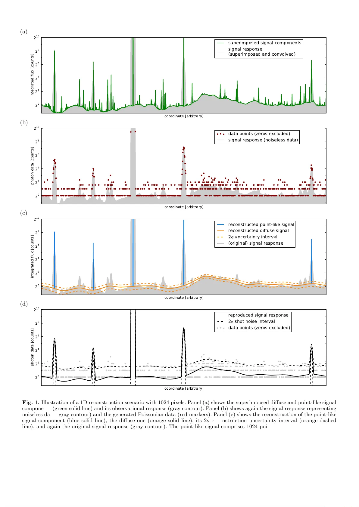
Astronom y & Astroph ysics man uscript no. D3PO c  ESO 2018 Octob er 15, 2018 Denoising, Deconvolving, and Decomp osing Photon Observations Derivation of the D 3 PO Algo rithm Marco Selig 1 , 2 and T orsten A. Enßlin 1 , 2 1 Max Planc k Institut für Astroph ysik (Karl-Sch w arzsc hild-Straße 1, D-85748 Garching, Germany) 2 Ludwig-Maximilians-Univ ersität München (Gesch wister-Sc holl-Platz 1, D-80539 München, Germany) Receiv ed 07 No v. 2013 / Accepted DD MMM. YYYY ABSTRA CT The analysis of astronomical images is a non-trivial task. The D 3 PO algorithm addresses the inference problem of denoising, decon v olving, and decomp osing photon observ ations. Its primary goal is the sim ultaneous but individual reconstruction of the diffuse and p oint-lik e photon flux given a single photon coun t image, where the fluxes are sup er- imp osed. In order to discriminate betw een these morphologically differen t signal comp onen ts, a probabilistic algorithm is derived in the language of information field theory based on a hierarc hical Bay esian parameter mo del. The signal inference exploits prior information on the spatial correlation structure of the diffuse comp onent and the brigh tness distribution of the spatially uncorrelated p oin t-lik e sources. A maximum a p osteriori solution and a solution minimizing the Gibbs free energy of the inference problem using v ariational Bay esian metho ds are discussed. Since the deriv ation of the solution is not dep endent on the underlying p osition space, the implementation of the D 3 PO algorithm uses the NIFTy pack age to ensure applicabilit y to v arious spatial grids and at any resolution. The fidelity of the algorithm is v al- idated by the analysis of simulated data, including a realistic high energy photon coun t image sho wing a 32 × 32 arcmin 2 observ ation with a spatial resolution of 0 . 1 arcmin . In all tests the D 3 PO algorithm successfully denoised, deconv olv ed, and decomp osed the data in to a diffuse and a point-lik e signal estimate for the respective photon flux comp onents. Key w o rds. metho ds: data analysis – metho ds: n umerical – metho ds: statistical – tec hniques: image processing – gamma-ra ys: general – X-rays: general 1. Intro duction An astronomical image migh t displa y m ultiple sup erim- p osed features, suc h as p oint sources, compact ob jects, dif- fuse emission, or background radiation. The ra w photon coun t images delivered by high energy telescop es are far from p erfect; they suffer from shot noise and distortions caused by instrumen tal effects. The analysis of suc h astro- nomical observ ations demands elab orate denoising, decon- v olution, and decomp osition strategies. The data obtained b y the detection of individual pho- tons is sub ject to P oissonian shot noise which is more severe for lo w coun t rates. This causes difficulty for the discrim- ination of fain t sources against noise, and makes their de- tection exceptionally challenging. F urthermore, unev en or incomplete survey co verage and complex instrumen tal re- sp onse functions lea ve imprints in the photon data. As a result, the data set migh t exhibit gaps and artificial distor- tions rendering the clear recognition of different features a difficult task. Poin t-like sources are especially afflicted b y the instrumen t’s p oin t spread function (PSF) that smooths them out in the observed image, and therefore can cause fain ter ones to v anish completely in the background noise. In addition to such noise and conv olution effects, it is the sup erp osition of the different ob jects that mak es their sep- aration am biguous, if p ossible at all. In astrophysics, pho- ton emitting ob jects are commonly divided into tw o mor- phological classes, diffuse sources and p oint sources. Dif- fuse sources span rather smo othly across large fractions of an image, and exhibit apparen t internal correlations. P oint sources, on the contrary , are lo cal features that, if observed p erfectly , w ould only app ear in one pixel of the image. In this w ork, w e will not distinguish b etw een diffuse sources and background, b oth are diffus e con tributions. Interme- diate cases, whic h are sometimes classified as extended or compact sources, are also not considered here. The question arises of ho w to reconstruct the original source con tributions, the individual signals, that caused the observed photon data. This task is an ill-p osed inv erse problem without a unique solution. There are a num b er of heuristic and probabilistic approaches that address the problem of denoising, decon v olution, and decomp osition in partial or simpler settings. SExtra ctor (Bertin & Arnouts 1996) is one of the heuristic to ols and the most prominen t for iden tifying sources in astronomy . Its p opularity is mostly based on its sp eed and easy op erabilit y . Ho wev er, SExtractor pro- duces a catalog of fitted sources rather than denoised and decon v olv ed signal estimates. CLEAN (Högbom 1974) is commonly used in radio astronomy and attempts a decon- v olution assuming there are only contributions from p oint sources. Therefore, diffuse emission is not optimally recon- structed in the analysis of real observ ations using CLEAN . Article num ber, page 1 of 22 A&A pro ofs: man uscript no. D3PO coordinate [arbitrary] 2 0 2 2 2 4 2 6 2 8 2 1 0 integrated flux [counts] superimposed signal components signal response (superimposed and convolved) (a) coordinate [arbitrary] 2 0 2 2 2 4 2 6 2 8 2 1 0 photon data [counts] data points (zeros excluded) signal response (noiseless data) (b) coordinate [arbitrary] 2 0 2 2 2 4 2 6 2 8 2 1 0 integrated flux [counts] reconstructed point-like signal reconstructed diffuse signal 2 u n c e r t a i n t y i n t e r v a l (original) signal response (c) coordinate [arbitrary] 2 0 2 2 2 4 2 6 2 8 2 1 0 photon data [counts] reproduced signal response 2 s h o t n o i s e i n t e r v a l data points (zeros excluded) (d) Fig. 1. Illustration of a 1D reconstruction scenario with 1024 pixels. Panel (a) sho ws the sup erimp osed diffuse and point-lik e signal comp onen ts (green solid line) and its observ ational response (gra y con tour). Panel (b) shows again the signal resp onse representing noiseless data (gray contour) and the generated P oissonian data (red markers). Panel (c) sho ws the reconstruction of the p oint-lik e signal comp onent (blue solid line), the diffuse one (orange solid line), its 2 σ reconstruction uncertaint y int erv al (orange dashed line), and again the original signal response (gray contour). The p oint-lik e signal comprises 1024 point-sources of which only five are not to o faint. P anel (d) shows the repro duced signal resp onse representing noiseless data (black solid line), its 2 σ shot noise in terv al (blac k dashed line), and again the data (gra y mark ers). Article num ber, page 2 of 22 Marco Selig and T orsten A. Enßlin: D 3 PO – Denoising, Deconv olving, and Decomposing Photon Observ ations Multiscale extensions of CLEAN (Cornw ell 2008; Rau & Corn w ell 2011) impro ve on this, but are also not prefect (Junklewitz et al. 2013). Decomp osition tec hniques for dif- fuse bac kgrounds, based on the analysis of angular p o w er sp ectra ha v e recen tly b een prop osed b y Hensley et al. (2013). Inference methods, in contrast, inv estigate the proba- bilistic relation b etw een the data and the signals. Here, the signals of in terest are the different source contributions. Probabilistic approac hes allow a transparent incorp oration of mo del and a priori assumptions, but often result in com- putationally hea vier algorithms. As an initial attempt, a maxim um lik eliho o d analysis w as proposed b y V aldes (1982). In later w ork, maximum en trop y (Strong 2003) and minimum χ 2 metho ds (e.g., Bouc het et al. 2013) w ere applied to the INTEGRAL/SPI data reconstructing a single signal component, though. On the basis of sparse regularization a num b er of tec hniques ex- ploiting w av eforms (based on the work by Haar 1910, 1911) ha v e prov en successful in p erforming denoising and decon- v olution tasks in differen t settings (González-Nuevo et al. 2006; Willett & Now ak 2007; Dup e et al. 2009; Figueiredo & Bioucas-Dias 2010; Dupé et al. 2011). F or example, Schmitt et al. (2010, 2012) analyzed simulated (single and m ulti- c hannel) data from the F ermi γ -ray space telescope fo cus- ing on the remo v al of P oisson noise and decon volution or bac kground separation. F urthermore, a (generalized) mor- phological comp onent analysis denoised, deconv olved and decomp osed simulated radio data assuming Gaussian noise statistics (Bobin et al. 2007; Chapman et al. 2013). Still in the regime of Gaussian noise, Gio v annelli & Coulais (2005) derived a decon v olution algorithm for point and extended sources minimizing regularized least squares. They introduce an efficien t conv ex regularization sc heme at the price of a priori unmotiv ated fine tuning parameters. The fast algorithm P ow ellSnakes I/I I b y Carv alho et al. (2009, 2012) is capable of analyzing multi-frequency data sets and detecting p oin t-lik e ob jects within diffuse emission regions. It relies on matched filters using PSF templates and Ba y esian filters exploiting, among others, priors on source p osition, size, and n umber. P ow ellSnakes I I has b een suc- cessfully applied to the Planc k data (Planck Collaboration et al. 2011). The approach closest to ours is the bac kground-source separation tec hnique used to analyze the ROSA T data (Guglielmetti et al. 2009). This Ba yesian model is based on a tw o-comp onent mixture mo del that reconstructs ex- tended sources and (diffuse) bac kground concurrently . The latter is, how ever, describ ed by a spline mo del with a small n um b er of spline sampling p oin ts. The strategy presen ted in this work aims at the si- m ultaneous reconstruction of t w o signals, the diffuse and p oin t-lik e photon flux. Both fluxes contribute equally to the observ ed photon counts, but their morphological imprin ts are very different. The prop osed algorithm, deriv ed in the framew ork of information field theory (IFT) (Enßlin et al. 2009; Enßlin 2013), therefore incorporates prior assump- tions in form of a hierarchical parameter model. The fun- damen tally different morphologies of diffuse and p oint-lik e con tributions reflected in different prior correlations and statistics. The exploitation of these differen t prior models is crucial to the signal decomposition. In this w ork, w e exclu- siv ely consider Poissonian noise, in particular, but not ex- clusiv ely , in the low coun t rate regime, where the signal-to- noise ratio b ecomes challengingly low. The D 3 PO algorithm presen ted here targets the simultaneous denoising, deconv o- lution, and decomp osition of photon observ ations in to tw o signals, the diffuse and p oint-lik e photon flux. This task in- cludes the reconstruction of the harmonic p ow er spectrum of the diffuse comp onent from the data themselves. More- o v er, the prop osed algorithm provides a p osteriori uncer- tain t y information on b oth inferred signals. The fluxes from diffuse and p oint-lik e sources contribute equally to the observed photon coun ts, but their morpho- logical imprin ts are very different. The prop osed algorithm, deriv ed in the framework of information field theory (IFT) (Enßlin et al. 2009; Enßlin 2013, 2014), therefore incorp o- rates prior assumptions in form of a hierarc hical parameter mo del. The fundamentally differen t morphologies of diffuse and point-lik e con tributions reflected in different prior cor- relations and statistics. The exploitation of these differen t prior mo dels is k ey to the signal decomp osition. The diffuse and p oin t-lik e signal are treated as tw o sepa- rate signal fields. A signal field represen ts an original signal app earing in nature; e.g., the physical photon flux distribu- tion of one source comp onent as a function of real space or sky p osition. In theory , a field has infinitely many degrees of freedom b eing defined on a con tinuous position space. In computational practice, how ever, a field needs of course to b e defined on a finite grid. It is desirable that the signal field is reconstructed indep endently from the grid’s resolu- tion, except for p oten tially unresolv able features. 1 W e note that the point-lik e signal field hosts one point source in ev- ery pixel, how ever, most of them migh t be invisibly fain t. Hence, a complicated determination of the n umber of p oint sources, as many algorithms p erform, is not required in our case. The deriv ation of the algorithm mak es use of a wide range of Bay esian metho ds that are discussed b elow in de- tail with regard to their implications and applicabilit y . F or no w, let us consider an example to emphasize the range and performance of the D 3 PO algorithm. Figure 1 illus- trates a reconstruction scenario in one dimension, where the co ordinate could be an angle or p osition (or time, or energy) in order to represent a 1D sky (or a time series, or an energy spectrum). The numerical implem en tation uses the NIFTy 2 pac k age (Selig et al. 2013). NIFTy p ermits an algorithm to b e set up abstractly , independent of the finally c hosen top ology , dimension, or resolution of the un- derlying position space. In this wa y , a 1D prototype co de can be used for dev elopment, and then just be applied in 2D, 3D, or ev en on the sphere. The remainder of this paper is structured as follows. Sec. 2 discusses the inference on photon observ ations; i.e., the underlying model and prior assumptions. The D 3 PO al- gorithm solving this inference problem by denoising, decon- 1 If the resolution of the reconstruction were increased gradu- ally , the diffuse signal field might exhibit more and more small scale features until the information conten t of the given data is exhausted. F rom this p oint on, any further increase in resolution w ould not change the signal field reconstruction significantly . In a similar manner, the localization accuracy and num b er of de- tections of p oint sources might increase with the resolution until all relev ant information of the data was captured. All higher res- olution grids can then be regarded as acceptable represen tations of the con tin uous p osition space. 2 NIFTy homepage http://www.mpa- garching.mpg.de/ift/ nifty/ Article num ber, page 3 of 22 A&A pro ofs: man uscript no. D3PO v olution, and decomp osition is derived in Sec. 3. In Sec. 4 the algorithm is demons trated in a numerical application on sim ulated high energy photon data. W e conclude in Sec. 5. 2. Inference on photon observations 2.1. Signal inference Here, a signal is defined as an unknown quan tity of in terest that we wan t to learn ab out. The most imp ortant informa- tion source on a signal is the data obtained in an observ ation to measure the signal. Infe rring a signal from an observ a- tional data set poses a fundamental problem because of the presence of noise in the data and the ambiguit y that several p ossible signals could ha ve produced the same data, ev en in the case of negligible noise. F or example, given some image data like photon counts, w e wan t to infer the underlying photon flux distribution. This ph ysical flux is a contin uous scalar field that v aries with resp ect to time, energy , and observ ational position. The measured photon count data, how ever, is restricted by its spatial and energy binning, as w ell as its limitations in energy range and observ ation time. Basically , all data sets are finite for practical reasons, and therefore cannot capture all of the infinitely many degrees of freedom of the underlying con tin uous signal field. There is no exact solution to such signal inference prob- lems, since there might b e (infinitely) many signal field con- figurations that could lead to the same data. This is why a probabilistic data analysis, which do es not pretend to calcu- late the correct field configuration but provides exp ectation v alues and uncertain ties of the signal field, is appropriate for signal inference. Giv en a data set d , the a p osteriori probability distri- bution P ( s | d ) judges how likely a p otential signal s is. This p osterior is giv en b y Ba y es’ theorem, P ( s | d ) = P ( d | s ) P ( s ) P ( d ) , (1) as a combination of the likelihoo d P ( d | s ) , the signal prior P ( s ) , and the evidence P ( d ) , whic h serv es as a normaliza- tion. The lik eliho o d characterizes how lik ely it is to mea- sure data set d from a given signal field s . It co vers all pro cesses that are relev an t for the measurement of d . The prior describ es the kno wledge ab out s without considering the data, and should, in general, be less restrictiv e than the lik eliho o d. IFT is a Bay esian framew ork for the inference of sig- nal fields exploiting mathematical methods for theoretical ph ysics. A signal field, s = s ( x ) , is a function of a contin u- ous position x in some p osition space Ω . In order to a void a dep endence of the reconstruction on the partition of Ω , the according calculus regarding fields is geared to preserve the con tin uum limit (Enßlin 2013, 2014; Selig et al. 2013). In general, w e are in terested in the a p osteriori mean estimate m of the signal field given the data, and its (uncertaint y) co v ariance D , defined as m = h s i ( s | d ) = Z D s s P ( s | d ) , (2) D =  ( m − s )( m − s ) †  ( s | d ) , (3) where † denotes adjunction and h · i ( s | d ) the expectation v alue with respect to the posterior probability distribution P ( s | d ) . 3 In the following, the p osterior of the ph ysical photon flux distribution of tw o morphologically different source comp onen ts given a data set of photon counts is build up piece b y piece according to Eq. (1). 2.2. P oissonian lik eliho o d The images provided by astronomical high energy tele- scop es typically consist of integer photon coun ts that are binned spatially into pixels. Let d i b e the num b er of de- tected photons, also called even ts, in pixel i , where i ∈ { 1 , . . . , N pix } ⊂ N . The kind of signal field we would lik e to infer from such data is the causativ e photon flux distribution. The photon flux, ρ = ρ ( x ) , is defined for eac h position x on the observ a- tional space Ω . In astrophysics, this space Ω is t ypically the S 2 sphere representing an all-sky view, or a region within R 2 represen ting an appro ximately plane patch of the sky . The flux ρ migh t express different morphological features, whic h can b e classified in to a diffuse and p oint-lik e compo- nen t. The exact definitions of the diffuse and point-lik e flux should b e sp ecified a priori , without knowledge of the data, and are addressed in Sec. 2.3.1 and 2.3.3, respectively . At this point it shall suffices to sa y that the diffuse flux v aries smo othly on large spatial scales, while the flux originating from point sources is fairly local. These tw o flux compo- nen ts are sup erimp osed, ρ = ρ diffuse + ρ point − like = ρ 0 (e s + e u ) , (4) where we in tro duced the dimensionless diffuse and p oint- lik e signal fields, s and u , and the constant ρ 0 whic h absorbs the physical dimensions of the photon flux; i.e., even ts p er area p er energy and time in terv al. The exp onential function in Eq. (4) is applied comp onent wise. In this wa y , w e natu- rally account for the strict p ositivity of the photon flux at the price of a non-linear change of v ariables, from the flux to its natural logarithm. A measurement apparatus observing the photon flux ρ is expected to detect a certain num b er of photons λ . This pro cess can b e mo deled b y a linear response op erator R 0 as follo ws, λ = R 0 ρ = R (e s + e u ) , (5) where R = R 0 ρ 0 . This reads for pixel i , λ i = Z Ω d x R i ( x )  e s ( x ) + e u ( x )  . (6) The resp onse op erator R 0 comprises all asp ects of the mea- suremen t process; i.e., all instrumen t resp onse functions. This includes the surv ey cov erage, whic h describ es the in- strumen t’s o v erall exp osure to the observ ational area, and the instrumen t’s PSF, which describ es how a p oint source is imaged b y the instrumen t. The sup erp osition of different comp onen ts and the tran- sition from con tinuous coordinates to some discrete pix- elization, cf. Eq. (6), cause a severe loss of information 3 This exp ectation v alue is computed by a path integral, R D s , o ver the complete phase space of the signal field s ; i.e., all p os- sible field configurations. Article num ber, page 4 of 22 Marco Selig and T orsten A. Enßlin: D 3 PO – Denoising, Deconv olving, and Decomposing Photon Observ ations ab out the original signal fields. In addition to that, mea- suremen t noise distorts the signal’s imprin t in the data. The individual photon counts p er pixel can be assumed to follo w a Poisson distribution P each. Therefore, the likeli- ho o d of the data d given an exp ected num b er of ev en ts λ is mo deled as a product of statistically independent Poisson pro cesses, P ( d | λ ) = Y i P ( d i , λ i ) = Y i 1 d i ! λ d i i e − λ i . (7) The Poisson distribution has a signal-to-noise ratio of √ λ whic h scales with the exp ected num b er of photon coun ts. Therefore, P oissonian shot noise is most sev ere in regions with lo w photon fluxes. This makes the detection of fain t sources in high energy astronomy a particularly challenging task, as X- and γ -ray photons are sparse. The likelihoo d of photon count data given a t w o comp o- nen t photon flux is hence describ ed by the Eqs. (5) and (7). Rewriting this lik eliho o d P ( d | s , u ) in form of its negative logarithm yields the information Hamiltonian H ( d | s , u ) , 4 H ( d | s , u ) = − log P ( d | s , u ) (8) = H 0 + 1 † λ − d † log( λ ) (9) = H 0 + 1 † R (e s + e u ) − d † log ( R (e s + e u )) , (10) where the ground state energy H 0 comprises all terms con- stan t in s and u , and 1 is a constan t data v ector b eing 1 ev erywhere. 2.3. Prio r assumptions The diffuse and p oint-lik e signal fields, s and u , contribute equally to the likelihoo d defined b y Eq. (10), and thus leav- ing it completely degenerate. On the mere basis of the likeli- ho o d, the full data set could be explained by the diffuse sig- nal alone, or only by p oint-sources, or any other conceiv able com bination. In order to down weigh t in tuitiv ely implausible solutions, we introduce priors. The priors discussed in the follo wing address the morphology of the differen t photon flux contributions, and define diffuse and p oint-lik e in the first place. These priors aid the reconstruction by pro vid- ing some remedy for the degeneracy of the lik eliho o d. The lik eliho o d describes noise and con volution properties, and the prior describ e the individual morphological prop erties. Therefore, the denoising and deconv olution of the data to- w ards the total photon flux ρ is primarily lik eliho o d driven, but for a decomp osition of the total photon flux in to ρ ( s ) and ρ ( u ) , the signal priors are imp erativ e. 2.3.1. Diffuse comp onent The diffuse photon flux, ρ ( s ) = ρ 0 e s , is strictly p ositive and migh t v ary in in tensit y ov er several orders of magnitude. Its morphology shows cloudy patc hes with smo oth fluctuations across spatial scales; i.e., one exp ects similar v alues of the diffuse flu x in neighboring lo cations. In other words, the dif- fuse comp onent exhibits spatial correlations. A log-normal mo del for ρ ( s ) satisfies those requiremen ts according to the 4 Throughout this work w e define H ( · ) = − log P ( · ) , and ab- sorb constan t terms in to a normalization constan t H 0 in fa vor of clarity . maxim um entrop y principle (Opp ermann et al. 2012; Kin- ney 2013). If the diffuse photon flux follows a multiv ariate log-normal distribution, the diffuse signal field s ob eys a m ultiv ariate Gaussian distribution G , P ( s | S ) = G ( s , S ) = 1 p det[2 π S ] exp  − 1 2 s † S − 1 s  , (11) with a giv en co v ariance S =  ss †  ( s | S ) . This co v ariance describ es the strength of the spatial correlations, and thus the smo othness of the fluctuations. A con v enien t parametrization of the cov ariance S can b e found, if the signal field s is a priori not known to distin- guish any p osition or orien tation axis; i.e., its correlations only depend on relative distances. This is equiv alent to as- sume s to b e statistically homogeneous and isotropic. Under this assumption, S is diagonal in the harmonic basis 5 of the p osition space Ω suc h that S = X k e τ k S k , (12) where τ k are spectral parameters and S k are pro jections on to a set of disjoint harmonic subspaces of Ω . These sub- spaces are commonly denoted as sp ectral bands or harmonic mo des. The set of sp ectral parameters, τ = { τ k } k , is the n the logarithmic p o w er sp ectrum of the diffuse signal field s with resp ect to the c hosen harmonic basis denoted by k . Ho w ev er, the diffuse signal cov ariance is in general un- kno wn a priori . This requires the introduction of another prior for the cov ariance, or for the set of parameters τ describing it adequately . This approach of h yp erpriors on prior parameters creates a hierarc hical parameter mo del. 2.3.2. Unkno wn p o w er sp ectrum The lac k of knowledge of the p ow er sp ectrum, requires its reconstruction from the same data the signal is inferred from (W andelt et al. 2004; Jasc he et al. 2010; Enßlin & F rommert 2011; Jasche & W andelt 2013). Therefore, tw o a priori constrain ts for the sp ectral parameters τ , whic h describ e the logarithmic pow er sp ectrum, are incorp orated in the mo del. The pow er sp ectrum is unkno wn and migh t span o v er sev eral orders of magnitude. This implies a logarithmically uniform prior for each element of the p ow er spectrum, and a uniform prior for each sp ectral parameter τ k , resp ectively . W e initially assume indep endent inv erse-Gamma distribu- tions I for the individual elemen ts, P (e τ | α , q ) = Y k I (e τ k , α k , q k ) (13) = Y k q α k − 1 k Γ( α k − 1) e − ( α k τ k + q k e − τ k ) , (14) and hence P un ( τ | α , q ) = Y k I (e τ k , α k , q k )     de τ k d τ k     (15) ∝ exp  − ( α − 1 ) † τ − q † e − τ  , (16) 5 The basis in which the Laplace op erator is diagonal is denoted harmonic basis. If Ω is a n -dimensional Euclidean space R n or T orus T n , the harmonic basis is the F ourier basis; if Ω is the S 2 sphere, the harmonic basis is the spherical harmonics basis. Article num ber, page 5 of 22 A&A pro ofs: man uscript no. D3PO where α = { α k } k and q = { q k } k are the shap e and scale parameters, and Γ denotes the Gamma function. In the limit of α k → 1 and q k → 0 ∀ k , the in v erse-Gamma distri- butions b ecome asymptotically flat on a logarithmic scale, and th us P un constan t. 6 Small non-zero scale parameters, 0 < q k , pro vide lo wer limits for the p ow er spectrum that, in practice, lead to more stable inference algorithms. So far, the v ariability of the individual elements of the p ow er spectrum is accounted for, but the question ab out their correlations has not b een addressed. Empir- ically , p ow er sp ectra of a diffuse signal field do not ex- hibit wild fluctuation or c hange drastically ov er neighboring mo des. They rather sho w some sort of sp ectral smo othness. Moreo v er, for diffuse signal fields that were shaped b y lo cal and causal pro cesses, we might exp ect a finite correlation supp ort in position space. This translates in to a smooth p o w er sp ectrum. In order to incorp orate spectral smo oth- ness, w e emplo y a prior in tro duced by Enßlin & F rommert (2011); Oppermann et al. (2012). This prior is based on the second logarithmic deriv ative of the spectral parameters τ , and fa v ors p o w er sp ectra that ob ey a p o w er law. It reads P sm ( τ | σ ) ∝ exp  − 1 2 τ † T τ  , (17) with τ † T τ = Z d(log k ) 1 σ 2 k  ∂ 2 τ k ∂ (log k ) 2  2 , (18) where σ = { σ k } k are Gaussian standard deviations sp eci- fying the tolerance against deviation from a p ow er-law be- ha vior of the p ow er sp ectrum. A choice of σ k = 1 ∀ k w ould t ypically allo w for a c hange in the p o w er la w’s slop e of 1 p er e-fold in k . In the limit of σ k → ∞ ∀ k , no smo othness is enforced up on the p o w er sp ectrum. The resulting prior for the sp ectral parameters is given b y the pro duct of the priors discussed ab o v e, P ( τ | α , q , σ ) = P un ( τ | α , q ) P sm ( τ | σ ) . (19) The parameters α , q and σ are considered to b e giv en as part of the hierarc hical Ba y esian mo del, and provide a flex- ible handle to mo del our knowledge on the scaling and smo othness of the p o w er sp ectrum. 2.3.3. P oint-lik e comp onent The point-lik e photon flux, ρ ( u ) = ρ 0 e u , is supp osed to originate from very distant astrophysical sources. These sources appear morphologically point-lik e to an observer b ecause their actual extent is negligible given the extreme distances. This renders p oint sources to b e spatially lo cal phenomena. The photon flux con tributions of neighboring p oin t sources can (to zeroth order approximation) b e as- sumed to b e statistically indep enden t of eac h other. Ev en if the tw o sources are very close on the observ ational plane, their ph ysical distance migh t b e h uge. Even in practice, the spatial cross-correlation of p oin t sources is negligible. Therefore, statistically indep endent priors for the photon flux contribution of eac h point-source are assumed in the follo wing. 6 If P ( τ k = log z ) = const . , then a substitution yields P ( z ) = P (log z ) | d(log z ) / d z | ∝ z − 1 ∼ I ( z , α → 1 , q → 0) . Because of the spatial locality of a point source, the corresp onding photon flux signal is supp osed to b e confined to a single spot, to o. If the p oin t-lik e signal field, defined o v er a con tin uous p osition space Ω , is discretized properly 7 , this sp ot is sufficiently identified by an image pixel in the reconstruction. A discretization, ρ ( x ∈ Ω) → ( ρ x ) x , is an inevitable step since the algorithm is to b e implemented in a computer en vironmen t anyw ay . Nevertheless, w e hav e to ensure that the a priori assumptions do not dep end on the c hosen discretization but satisfy the con tin uous limit. Therefore, the prior for the p oint-lik e signal comp onent factorizes spatially , P ( ρ ( u ) ) = Y x P ( ρ ( u ) x ) , (20) but the functional form of the priors are y et to b e deter- mined. This mo del allows the point-lik e signal field to host one p oint source in every pixel. Most of these point sources are expected to b e in visibly fain t con tributing negligibly to the total photon flux. How ever, the point sources whic h are just iden tifiable from the data are pinpointed in the re- construction. In this approac h, there is no necessit y for a complicated determination of the num b er and p osition of sources. F or the construction of a prior, that the photon flux is a strictly positive quantit y also needs to b e considered. Thus, a simple exp onen tial prior, P ( ρ ( u ) x ) ∝ exp  − ρ ( u ) x /ρ 0  , (21) has been suggested (e.g., Guglielmetti et al. 2009). It has the adv antage of b eing (easily) analytically treatable, but its ph ysical implications are questionable. This distribution strongly suppresses high photon fluxes in fav or of low er ones. The maximum entrop y prior, which is also often ap- plied, is even w orse b ecause it corresp onds to a brigh tness distribution, 8 P ( ρ ( u ) x ) ∝  ρ ( u ) x /ρ 0  ( − ρ ( u ) x /ρ 0 ) . (22) The following (rather crude) consideration might motiv ate a more astroph ysical prior. Say the universe hosts a ho- mogeneous distribution of point sources. The n um b er of p oin t sources would therefore scale with the observ able v olume; i.e., with distance cubed. Their apparen t brigh t- ness, which is reduced b ecause of the spreading of the light ra ys; i.e., a prop ortionality to the distance squared. Conse- quen tly , a pow er-law b ehavior b etw een the num b er of point sources and their brigh tness with a slope β = 3 2 is to b e ex- p ected (F omalon t 1968; Malyshev & Hogg 2011). How ever, suc h a plain p o w er law diverges at 0 , and is not necessar- ily normalizable. F urthermore, Galactic and extragalactic sources cannot be found in arbitrary distances o wing to the finite size of the Galaxy and the cosmic (past) ligh t cone. Imp osing an exp onential cut-off ab ov e 0 onto the p o w er law yields an inv erse-Gamma distribution, which has b een shown to b e an appropriate prior for p oint-lik e photon fluxes (Guglielmetti et al. 2009; Carv alho et al. 2009, 2012). 7 The numerical discretization of information fields is describ ed in great detail in Selig et al. (2013). 8 The so-called maxim um entrop y regularization P x ( ρ ( u ) x /ρ 0 ) log ( ρ ( u ) x /ρ 0 ) of the log-likelihoo d can b e regarded as log-prior, cf. Eqs. (20) and (22). Article num ber, page 6 of 22 Marco Selig and T orsten A. Enßlin: D 3 PO – Denoising, Deconv olving, and Decomposing Photon Observ ations The prior for the p oin t-lik e signal field is therefore de- riv ed from a pro duct of indep endent inv erse-Gamma distri- butions, 9 P ( ρ ( u ) | β , η ) = Y x I ( ρ ( u ) x , β x , ρ 0 η x ) (23) = Y x ( ρ 0 η x ) β x − 1 Γ( β x − 1)  ρ ( u ) x  − β x exp − ρ 0 η x ρ ( u ) x ! , (24) yielding P ( u | β , η ) = Y x I ( ρ 0 e u x , β k , ρ 0 η k )     d ρ 0 e u x d u x     (25) ∝ exp  − ( β − 1 ) † u − η † e − u  , (26) where β = { β x } x and η = { η x } x are the shap e and scale parameters. The latter is resp onsible for the cut-off of v an- ishing fluxes, and should b e chosen adequately small in analogy to the sp ectral scale parameters q . The determina- tion of the shape parameters is more difficile. The geomet- rical argument ab ov e suggests a universal shap e parameter, β x = 3 2 ∀ x . A second argumen t for this v alue results from demanding a priori indep endence of the discretization. If w e c ho ose a coarser resolution that would add up the flux from t wo p oint sources at merged pixels, then our prior should still b e applicable. The univ ersal v alue of 3 2 indeed fulfills this requirement as sho wn in App endix A. There it is also shown that η has to b e c hosen resolution dep endent, though. 2.4. P a rameter mo del Figure 2 giv es an o v erview of the parameter hierarc hy of the suggested Bay esian mo del. The data d is given, and the diffuse signal field s and the p oint-lik e signal field u shall b e reconstructed from that data. The logarithmic pow er sp ectrum τ is a set of nuisance parameters that also need to be reconstructed from the data in order to accurately mo del the diffuse flux contributions. The model parameters form the top lay er of this hierarc hy and are given to the reconstruction algorithm. This set of mo del parameters can b e b oiled down to five scalars, namely α , q , σ , β , and η , if one defines α = α 1 , etc. The incorporation of the scalars in the inference is p ossible in theory , but this would increase the computational complexit y dramatically . W e discussed reasonable v alues for these scalars to b e c hosen a priori . If additional information sources, such as theoretical p ow er spectra or ob ject catalogs, are a v ail- able the model parameters can b e adjusted accordingly . In Sec. 4, different parameter c hoices for the analysis of simu- lated data are in v estigated. 3. Denoising, deconvolution, and decomposition The likelihoo d mo del, describing the measuremen t pro cess, and the prior assumptions for the signal fields and the p ow er 9 A p ossible extension of this prior mo del that includes spa- tial correlations would b e an in verse-Wishart distribution for diag[ ρ ( u ) ] . α, q σ β , η τ s u ρ λ d Fig. 2. Graphical model of the mo del parameters α , q , σ , β , and η , the logarithmic spectral parameters τ , the diffuse signal field s , the point-lik e signal field u , the total photon flux ρ , the exp ected n umber of photons λ , and the observed photon coun t data d . sp ectrum of the diffuse comp onent yield a well-defined in- ference problem. The corresp onding p osterior is giv en b y P ( s , τ , u | d ) = P ( d | s , u ) P ( s | τ ) P ( τ | α, q , σ ) P ( u | β , η ) P ( d ) , (27) whic h is a complex form of Ba y es’ theorem (1). Ideally , we w ould no w calculate the a p osteriori exp ec- tation v alues and uncertain ties according to Eqs. (2) and (3) for the diffuse and p oint-lik e signal fields, s and u , as w ell as for the logarithmic sp ectral parameters τ . How ever, an analytical ev aluation of these exp ectation v alues is not p ossible b ecause of the complexit y of the p osterior. The p osterior is non-linear in the signal fields and, ex- cept for artificially constructed data, non-con vex. It, ho w- ev er, is more flexible and therefore allo ws for a more com- prehensiv e description of the parameters to be inferred (Kirkpatric k et al. 1983; Geman & Geman 1984). Numerical approac hes in v olving Mark ov c hain Monte Carlo metho ds (Metrop olis & Ulam 1949; Metrop olis et al. 1953) are p ossible, but hardly feasible b ecause of the h uge parameter phase space. Nevertheless, similar problems ha ve b een addressed by elaborate sampling techniques (W an- delt et al. 2004; Jasc he et al. 2010; Jasche & Kitaura 2010; Jasc he & W andelt 2013). Here, t wo appro ximative algorithms with low er compu- tational costs are deriv ed. The first one uses the maxim um a p osteriori (MAP) appro ximation, the second one mini- mizes the Gibbs free energy of an approximate posterior ansatz in the spirit of v ariational Ba y esian metho ds. The fidelit y and accuracy of these t wo algorithms are compared in a n umerical application in Sec. 4. 3.1. P osterio r maximum The p osterior maxim um and mean coincide, if the p osterior distribution is symmetric and single peaked. In practice, this often holds – at least in goo d approximation –, so that the maximum a p osteriori approach can provide suitable es- timators. This can either be achiev ed using a δ -distribution Article num ber, page 7 of 22 A&A pro ofs: man uscript no. D3PO at the p osterior’s mo de, h s i ( s | d ) MAP - δ ≈ Z D s s δ ( s − s mode ) , (28) or using a Gaussian appro ximation around this p oin t, h s i ( s | d ) MAP - G ≈ Z D s s G ( s − s mode , D mode ) , (29) Both appro ximations require us to find the mo de, which is done b y extremizing the p osterior. Instead of the complex p osterior distribution, it is con- v enien t to consider the information Hamiltonian, defined b y its negativ e logarithm, H ( s , τ , u | d ) = − log P ( s , τ , u | d ) (30) = H 0 + 1 † R (e s + e u ) − d † log ( R (e s + e u )) + 1 2 log (det [ S ]) + 1 2 s † S − 1 s (31) + ( α − 1 ) † τ + q † e − τ + 1 2 τ † T τ + ( β − 1 ) † u + η † e − u , where all terms constant in s , τ , and u hav e been absorb ed in to a ground state energy H 0 , cf. Eqs. (7), (11), (19), and (26), resp ectiv ely . The MAP solution, which maximizes the p osterior, min- imizes the Hamiltonian. This minim um can thus b e found b y taking the first (functional) deriv atives of the Hamil- tonian with resp ect to s , τ , and u and equating them with zero. Unfortunately , this yields a set of implicit, self-consisten t equations rather than an explicit solution. Ho w ev er, these equations can b e solved by an iterative minimization of the Hamiltonian using a steep est descent metho d for example, see Sec. 3.4 for details. In order to b etter understand the structure of the MAP solution, w e consider the minimum ( s , τ , u ) = ( m ( s ) , τ ? , m ( u ) ) . The resulting filter form ulas for the dif- fuse and p oin t-lik e signal field read ∂ H ∂ s     min = 0 = ( 1 − d / l ) † R ∗ e m ( s ) + S ? − 1 m ( s ) , (32) ∂ H ∂ u     min = 0 = ( 1 − d / l ) † R ∗ e m ( u ) + β − 1 − η ∗ e − m ( u ) , (33) with l = R  e m ( s ) + e m ( u )  , (34) S ? = X k e τ ? k S k . (35) Here, ∗ and / denote component wise m ultiplication and di- vision, resp ectively . The first term in Eq. (32) and (33), whic h comes from the lik eliho o d, v anishes in case l = d . W e note that l = λ | min describ es the most likely n um ber of photon counts, not the exp ected num b er of photon counts λ = h d i ( d | s , u ) , cf. Eqs. (5) and (7). Disregarding the reg- ularization by the priors, the solution w ould o verfit; i.e., noise features are partly assigned to the signal fields in or- der to achiev e an unnecessarily close agreement with the data. Ho wev er, the a priori regularization suppresses this tendency to some extend. The second deriv ativ e of the Hamiltonian describes the curv ature around the minimum, and therefore approxi- mates the (in v erse) uncertain t y co v ariance, ∂ 2 H ∂ s ∂ s †     min ≈ D ( s ) − 1 , ∂ 2 H ∂ u ∂ u †     min ≈ D ( u ) − 1 . (36) The closed form of D ( s ) and D ( u ) is giv en explicitly in App endix B. The filter form ula for the pow er sp ectrum, which is de- riv ed from a first deriv ativ e of the Hamiltonian with respect to τ , yields e τ ? = q + 1 2  tr h m ( s ) m ( s ) † S − 1 k i k γ + T τ ? , (37) where γ = ( α − 1 ) + 1 2  tr  S k S k − 1  k . This formula is in accordance with the results b y Enßlin & F rommert (2011); Opp ermann et al. (2012). It has been shown by the former authors that such a filter exhibits a p erception threshold; i.e., on scales where the signal-resp onse-to-noise ratio drops b elo w a certain bound the reconstructed signal pow er b e- comes v anishingly lo w. This threshold can b e cured b y a b etter capture of the a p osteriori uncertain ty structure. 3.2. P osterio r app ro ximation In order to o vercome the analytical infeasibility as well as the p erception threshold, we seek an appro ximation to the true posterior. Instead of approximating the expectation v alues of the p osterior, approximate p osteriors are in v es- tigated in this section. In case the appro ximation is goo d, the exp ectation v alues of the appro ximate posterior should then b e close to the real ones. The posterior given by Eq. (27) is inaccessible b ecause of the en tanglement of the diffuse signal field s , its loga- rithmic p ow er sp ectrum τ , and the point-lik e signal field u . The in volv ement of τ can been simplified b y a mean field appro ximation, P ( s , τ , u | d ) ≈ Q = Q s ( s , u | µ , d ) Q τ ( τ | µ , d ) , (38) where µ denotes an abstract mean field mediating some information betw een the signal field tuple ( s , u ) and τ that are separated b y the pro duct ansatz in Eq. (38). This mean field is fully determined b y the problem, as it represen ts effectiv e (rather than additional) degrees of freedom. It is only needed implicitly for the deriv ation, an explicit formula can b e found in App endix C.3, though. Since the a p osteriori mean estimates for the signal fields and their uncertaint y co v ariances are of primary in- terest, a Gaussian approximation for Q s that accoun ts for correlation betw een s and u would b e sufficien t. Hence, our previous appro ximation is extended b y setting Q s ( s , u | µ , d ) = G ( ϕ , D ) , (39) with ϕ =  s − m ( s ) u − m ( u )  , D = D ( s ) D ( su ) D ( su ) † D ( u ) ! . (40) Article num ber, page 8 of 22 Marco Selig and T orsten A. Enßlin: D 3 PO – Denoising, Deconv olving, and Decomposing Photon Observ ations This Gaussian appro ximation is also a con venien t c hoice in terms of computational complexit y b ecause of its simple analytic structure. The go o dness of the appro ximation P ≈ Q can b e quan tified by an information theoretical measure, see Ap- p endix C.1. The Gibbs free energy of the inference problem, G =  H ( s , τ , u | d )  Q −  − log Q ( s , τ , u | d )  Q , (41) whic h is equiv alent to the Kullbac k-Leibler divergence D KL ( Q, P ) , is chosen as such a measure (Enßlin & W eig 2010). In fav or of comprehensibilit y , we supp ose the solution for the logarithmic p ow er spectrum τ ? is known for the momen t. The Gibbs free energy is then calculated b y plug- ging in the Hamiltonian, and ev aluating the exp ectation v alues 10 , G = G 0 +  H ( s , u | d )  Q s − 1 2 log (det [ D ]) (42) = G 1 + 1 † l − d † ( log( l ) − ∞ X ν =2 ( − 1) ν ν  ( λ / l − 1) ν  Q s ) + 1 2 m ( s ) † S ? − 1 m ( s ) + 1 2 tr h D ( s ) S ? − 1 i (43) + ( β − 1 ) † m ( u ) + η † e − m ( u ) + 1 2 b D ( u ) − 1 2 log (det [ D ]) , with λ = R (e s + e u ) , (44) l = h λ i Q s = R  e m ( s ) + 1 2 b D ( s ) + e m ( u ) + 1 2 b D ( u )  , (45) S ? = X k e τ ? k S k , and (46) b D = diag [ D ] . (47) Here, G 0 and G 1 carry all terms indep endent of s and u . In comparison to the Hamiltonian given in Eq. (31), there are a n um b er of correction terms that now also c onsider the uncertain t y cov ariances of the signal estimates prop erly . F or example, the exp ectation v alues of the photon fluxes differ comparing l in Eq. (34) and (45) where it no w describ es the exp ectation v alue of λ o ver the appro ximate p osterior. In case l = λ the explicit sum in Eq. (43) v anishes. Since this sum includes p ow ers of  λ ν > 2  Q s its ev aluation w ould require all entries of D to b e known explicitly . In order to k eep the algorithm computationally feasible, this sum shall hereafter be neglected. This is equiv alent to truncating the corresp onding expansion at second order; i.e., ν = 2 . It can b e sho wn that, in consequence of this app ro ximation, the cross-correlation D ( su ) equals zero, and D becomes block diagonal. 10 The second lik eliho o d term in Eq. (43), d † log( λ ) , is thereb y expanded according to log( x ) = log h x i − ∞ X ν =2 ( − 1) ν ν  x h x i − 1  ν  ≈ log h x i + O  x 2  , under the assumption x ≈ h x i . Without these second order terms, the Gibbs free energy reads G = G 1 + 1 † l − d † log( l ) + 1 2 m ( s ) † S ? − 1 m ( s ) + 1 2 tr h D ( s ) S ? − 1 i (48) + ( β − 1 ) † m ( u ) + η † e − m ( u ) + 1 2 b D ( u ) − 1 2 log  det h D ( s ) i − 1 2 log  det h D ( u ) i . Minimizing the Gibbs free energy with resp ect to m ( s ) , m ( u ) , D ( s ) , and D ( u ) w ould optimize the fitness of the p osterior appro ximation P ≈ Q . Filter form ulas for the Gibbs solution can b e deriv ed b y taking the deriv ativ e of G with resp ect to the appro ximate mean estimates, ∂ G ∂ m ( s ) = 0 = ( 1 − d / l ) † R ∗ e m ( s ) + 1 2 b D ( s ) + S ? − 1 m ( s ) , (49) ∂ G ∂ m ( u ) = 0 = ( 1 − d / l ) † R ∗ e m ( u ) + 1 2 b D ( u ) (50) + β − 1 − η ∗ e − m ( u ) + 1 2 b D ( u ) , This filter formulas again account for the uncertaint y of the mean estimates in comparison to the MAP filter formulas in Eq. (32) and (33). The uncertain ty cov ariances can b e constructed b y either taking the second deriv atives, ∂ 2 G ∂ m ( s ) ∂ m ( s ) † ≈ D ( s ) − 1 , ∂ 2 G ∂ m ( u ) ∂ m ( u ) † ≈ D ( u ) − 1 , (51) or setting the first deriv ativ es of G with respect to the un- certain t y co v ariances equal to zero matrices, ∂ G ∂ D ( s ) xy = 0 , ∂ G ∂ D ( u ) xy = 0 . (52) The closed form of D ( s ) and D ( u ) is giv en explicitly in App endix B. So far, the logarithmic pow er sp ectrum τ ? , and with it S ? , hav e b een supp osed to be known. The mean field appro ximation in Eq. (38) do es not sp ecify the approximate p osterior Q τ ( τ | µ , d ) , but it can b e retriev ed b y v ariational Ba y esian methods (Jordan et al. 1999; Wingate & W eber 2013), according to the pro cedure detailed in App endix C.2. The subsequent Appendix C.3 discusses the deriv ation of an solution for τ by extremizing Q τ . This result, whic h w as also derived in Oppermann et al. (2012), applies to the inference problem discussed here, yielding e τ ? = q + 1 2  tr h m ( s ) m ( s ) † + D ( s )  S − 1 k i k γ + T τ ? . (53) Again, this solution includes a correction term in compar- ison to the MAP solution in Eq. (37). Since D ( s ) is p os- itiv e definite, it contributes p ositive to the (logarithmic) p o w er sp ectrum, and therefore reduces the possible p ercep- tion threshold further. W e note that this is a minimal Gibbs free energy so- lution that maximizes Q τ . A proper calculation of h τ i Q τ migh t include further correction terms, but their deriv ation Article num ber, page 9 of 22 A&A pro ofs: man uscript no. D3PO is not p ossible in closed form. Moreo ver, the abov e used dif- fuse signal cov ariance S ? − 1 should be replaced b y  S − 1  Q τ adding further correction terms to the filter form ulas. In order to keep the computational complexity on a fea- sible level, all these higher order corrections are not con- sidered here. The detailed characterization of their impli- cations and implemen tation difficulties is left for future in- v estigation. 3.3. Physical flux solution T o perform calculations on the logarithmic fluxes is con- v enien t for numerical reasons, but it is the physical fluxes that are actually of interest to us. Giv en the chosen appro xi- mation, we can compute the p osterior exp ectation v alues of the diffuse and p oint-lik e photon flux, ρ ( s ) and ρ ( u ) , straight forw ardly , D ρ ( · ) E P MAP - δ ≈ D ρ ( · ) E δ = ρ 0 e m ( · ) mode , (54) MAP - G ≈ D ρ ( · ) E G = ρ 0 e m ( · ) mode + 1 2 b D ( · ) mode , (55) Gibbs ≈ D ρ ( · ) E Q = ρ 0 e m ( · ) mean + 1 2 b D ( · ) mean , (56) in accordance with Eq. (28), (29), or (38), resp ectively . Those solutions differ from each other in terms of the in- v olv emen t of the p osterior’s mo de or mean, and in terms of the inclusion of the uncertain t y information, see subscripts. In general, the mo de appro ximation holds for symmet- ric, single p eaked distributions, but can p erform po orly in other cases (e.g., Enßlin & F rommert 2011). The exact form of the p osterior considered here is highly complex b ecause of the many degrees of freedom. In a dimensionally reduced frame, ho wev er, the p osterior app ears single p eaked and exhibits a negativ e skewness. 11 Although this is not neces- sarily generalizable, it suggest a sup eriority of the posterior mean compared to the MAP b ecause of the asymmetry of the distribution. Nev ertheless, the MAP approac h is com- putationally cheaper compared to the Gibbs approac h that requires permanent kno wledge of the uncertain ty co v ari- ance. The uncertaint y of the reconstructed photon flux can b e appro ximated as for an ordinary log-normal distribution, D ρ ( · ) 2 E P − D ρ ( · ) E 2 P MAP ≈ D ρ ( · ) E 2 G  e b D ( · ) mode − 1  , (57) Gibbs ≈ D ρ ( · ) E 2 Q  e b D ( · ) mean − 1  , (58) where the square ro ot of the latter term would describ e the relativ e uncertain t y . 3.4. Imaging algo rithm The problem of denoising, deconv olving, and decomp osing photon observ ations is a non-trivial task. Therefore, this section discusses the implementation of the D 3 PO algo- rithm giv en the t w o sets of filter form ulas derived in Sec. 3.1 and 3.2, resp ectiv ely . 11 F or example, the p osterior P ( s | d ) for a one-dimensional dif- fuse signal is prop ortional to exp( − 1 2 s 2 + ds − exp( s )) , whereby all other parameters are fixed to unity . Analogously , P ( u | d ) ∝ exp( du − 2 cosh( u )) . The information Hamiltonian, or equiv alen tly the Gibbs free energy , are scalar quan tities defined o v er a h uge phase space of p ossible field and parameter configurations includ- ing, among others, the elemen ts of m ( s ) and m ( u ) . If w e only consider those, and no resolution refinement from data to signal space, t w o num b ers need to b e inferred from one data v alue each. Including τ and the uncertaint y cov ari- ances D ( s ) and D ( u ) in the inference, the problem of un- derdetermined degrees of freedom gets w orse. This is re- flected in the p ossibilit y of a decen t num b er of lo cal minima in the non-con v ex manifold landscape of the co domain of the Hamiltonian, or Gibbs free energy , resp ectively (Kirk- patric k et al. 1983; Geman & Geman 1984; Giov annelli & Coulais 2005). The complexity of the inference problem go es back to the, in general, non-linear en tanglement b e- t w een the individual parameters. The D 3 PO algorithm is based on an iterativ e optimiza- tion scheme, where certain subsets of the problem are op- timized alternately instead of the full problem at once. Eac h subset optimization is designed individually , see be- lo w. The global optimization cycle is in some degree sensi- tiv e to the starting v alues b ecause of the non-con v exit y of the considered p otential; i.e., the information Hamiltonian or Gibbs free energy , resp ectiv ely . W e can find such appro- priate starting v alues by solving the inference problem in a reduced frame in adv ance, see b elow. So far, a step-b y-step guide of the algorithm lo oks lik e the follo wing. 1. Initialize the algorithm with primitive starting v alues; e.g., m ( s ) x = m ( u ) x = 0 , D ( s ) xy = D ( u ) xy = δ xy , and τ ? k = log( k − 2 ) . – Those v alues are arbitrary . Although the optimization is rather insensitiv e to them, inappro- priate v alues can cripple the algorithm for n umerical reasons b ecause of the high non-linearity of the infer- ence problem. 2. Optimize m ( s ) , the diffuse signal field, coarsely . – The preliminary optimization shall yield a rough estimate of the diffuse only contribution. This can b e ac hieved b y reconstructing a coarse screened diffuse signal field that only v aries on large scales; i.e., limiting the bandwidth of the diffuse signal in its harmonic basis. Alternativ ely , ob vious point sources in the data could b e mask ed out b y in tro ducing an artificial mask in to the response, if feasible. 3. Optimize m ( u ) , the p oin t-lik e signal field, lo cally . – This initial optimization shall appro ximate the bright- est, most ob vious, p oint sources that are visible in the data image by eye. Their curren t disagreement with the data dominates the considered p otential, and introduces some numerical stiffness. The gradien t of the p otential can b e computed according to Eq. (33) or (50), and its minima will b e at the exp ected p osition of the brightest p oin t source which has not b een reconstructed, yet. It is therefore v ery efficien t to increase m ( u ) at this lo cation directly until the sign of the gradient flips, and rep eat this pro cedure un til the ob vious p oin t sources are fit. 4. Optimize m ( u ) , the p oint-lik e signal field. – This task can b e done by a steep est descen t minimization of the p oten tial com bined with a line searc h following the W olfe conditions (Noce dal & W righ t 2006). The p oten- tials can be computed according to Eq. (31) or (43) neglecting terms indep endent of m ( u ) , and the gradien t according to Eq. (33) or (50). A more sophisticated min- imization sc heme, suc h as a non-linear conjugate gradi- Article num ber, page 10 of 22 Marco Selig and T orsten A. Enßlin: D 3 PO – Denoising, Deconv olving, and Decomposing Photon Observ ations (a) (b) (c) (d) (e) (f ) Fig. 3. Illustration of the data and noiseless, but reconv olved, signal responses of the reconstructions. Panel (a) sho ws the data from a mo ck observ ation of a 32 × 32 arcmin 2 patc h of the sky with a resolution of 0 . 1 arcmin corresponding to a total of 102 400 pixels. The data had been conv olved with a Gaussian-like PSF (FWHM ≈ 0 . 2 arcmin = 2 pixels, finite supp ort of 1 . 1 arcmin = 11 pixels) and mask ed b ecause of an uneven exp osure. Panel (b) shows the centered con v olution kernel. Panel (c) shows the exp osure mask. The b ottom panels show the recon volv ed signal resp onse R h ρ i of a reconstruction using a different approach each, namely (d) MAP- δ , (e) MAP- G , and (f ) Gibbs. All reconstructions sho wn here and in the follo wing figures used the same model parameters: α = 1 , q = 10 − 12 , σ = 10 , β = 3 2 , and η = 10 − 4 . en t (Shew ch uk 1994), is conceiv able but would require the application of the full Hessian, cf. step 5. In the first run, it might b e sufficient to restrict the optimization to the lo cations iden tified in step 3. 5. Up date b D ( u ) , the p oint-lik e uncertaint y v ariance, in case of a Gibbs approach. – It is not feasible to com- pute the full uncertain ty cov ariance D ( u ) explicitly in order to extract its diagonal. A more elegant wa y is to apply a probing tec hnique relying on the application of D ( u ) to random fields ξ that pro ject out the diagonal (Hutc hinson 1989; Selig et al. 2012). The uncertain ty co v ariance is given as the inv erse Hessian by Eq. (36) or (51), and should b e symmetric and p ositive definite. F or that reason, it can b e applied to a field using a conjugate gradien t (Shew ch uk 1994); i.e., solving ( D ( u ) ) − 1 y = ξ for y . Ho wev er, if the curren t phase space p osition is far a w a y from the minimum, the Hessian is not necessar- ily positive definite. One wa y to o v ercome this temp oral instabilit y , would be to introduce a Leven b erg damp- ing in the Hessian (inspired by T ranstrum et al. 2010; T ranstrum & Sethna 2012). 6. Optimize m ( s ) , the diffuse signal field. – An analog sc heme as in step 4 using steep est descent and W olfe conditions is effective. The potentials can b e computed according to Eq. (31) or (43) neglecting terms indep en- den t of m ( s ) , and the gradient according to Eq. (32) or (49), resp ectively . It has prov en useful to first ensure a con v ergence on large scales; i.e., small harmonic mo des k . This can b e done rep eating steps 6, 7, and 8 for all k < k max with gro wing k max using the corresp onding pro jections S k . 7. Up date b D ( s ) , the diffuse uncertain ty v ariance, in case of a Gibbs approac h in analogy to step 5. 8. Optimize τ ? , the logarithmic pow er sp ectrum. – This is done by solving Eq. (37) or (53). The trace term can b e computed analog to the diagonal; e.g., b y probing. Giv en this, the equation can b e solv ed efficien tly by a Newton-Raphson metho d. 9. Rep eat the steps 4 to 8 un til conv ergence. – This scheme will take several cycles un til the algorithm reaches the Article num ber, page 11 of 22 A&A pro ofs: man uscript no. D3PO (a) (b) (c) (d) (e) (f ) Fig. 4. Illustration of the diffuse reconstruction. The top panels sho w the denoised and deconv olved diffuse contribution h ρ ( s ) i /ρ 0 reconstructed using a different approach eac h, namely (d) MAP- δ , (e) MAP- G , and (f ) Gibbs. The bottom panels (d) to (f ) sho w the difference betw een the originally simulated signal and the respective reconstruction. desired con vergence lev el. Therefore, it is not required to achiev e a con vergence to the final accuracy level in all subsets in all cycles. It is advisable to start with w eak con v ergence criteria in the first lo op and increase them gradually . A few remarks are in order. The phase space of possible signal field configurations is tremendously huge. It is therefore impossible to judge if the algorithm has conv erged to the global or some lo cal minima, but this does not matter if b oth yield reasonable results that do not differ substan tially . In general, the conv erged solution is also sub ject to the c hoice of starting v alues. Solving a non-conv ex, non-linear inference problem without proper initialization can easily lead to nonsensical results, such as fitting (all) diffuse fea- tures by p oin t sources. Therefore, the D 3 PO algorithm es- sen tially creates its own starting v alues executing the ini- tial steps 1 to 3. The primitive starting v alues are thereby pro cessed to rough estimates that cov er coarsely resolv ed diffuse and prominen t point-lik e features. These estimates serv e then as actual starting v alues for the optimization cycle. Because of the iterative optimization sc heme starting with the diffuse comp onent in step 2, the algorithm might b e prone to explaining some p oint-lik e features b y diffuse sources. Starting with the p oint-lik e comp onent instead w ould give rise to the opp osite bias. T o av oid such biases, it is advisable to restart the algorithm partially . T o be more precise, w e prop ose to discard the current reconstruction of m ( u ) after finishing step 8 for the first time, then start the second iteration again with step 3, and to discard the curren t m ( s ) b efore step 6. The ab ov e scheme exploits a few numerical tec hniques, suc h as probing or Leven b erg damping, that are describ ed in great detail in the given references. The code of our im- plemen tation of the D 3 PO algorithm will be made public in the future under http://www.mpa- garching.mpg.de/ ift/d3po/ . 4. Numerical application Exceeding the simple 1D scenario illustrated in Fig. 1, the D 3 PO algorithm is no w applied to a realistic, but sim u- lated, data set. The data set represents a high energy ob- serv ation with a field of view of 32 × 32 arcmin 2 and a reso- lution of 0 . 1 arcmin ; i.e., the photon count image comprises 102 400 pixels. The instrument resp onse includes the con v o- lution with a Gaussian-like PSF with a FWHM of roughly Article num ber, page 12 of 22 Marco Selig and T orsten A. Enßlin: D 3 PO – Denoising, Deconv olving, and Decomposing Photon Observ ations (a) (b) (c) (d) = (a) − (b) (e) = (a) − (c) (f ) = | (e) | / (c) (g) (h) Fig. 5. Illustration of the reconstruction of the diffuse signal field s = log ρ ( s ) and its uncertaint y . The top panels show diffuse signal fields. P anel (a) shows the original sim ulation s , panel (b) the reconstruction m ( s ) mode using a MAP approach, and panel (c) the reconstruction m ( s ) mean using a Gibbs approach. The panels (d) and (e) show the differences b etw een original and reconstruction. P anel (f ) sho ws the relative difference. The panels (g) and (h) show the relativ e uncertain ty of the ab ov e reconstructions. 0 . 2 arcmin , and an uneven survey mask attributable to the inhomogeneous exp osure of the virtual instrument. The data image and those c haracteristics are sho wn in Fig. 3. In addition, the top panels of Fig. 3 show the repro duced signal responses of the reconstructed (total) photon flux. The reconstructions used the same mo del parameters, α = 1 , q = 10 − 12 , σ = 10 , β = 3 2 , and η = 10 − 4 in a MAP- δ , MAP- G and a Gibbs approach, respectively . They all show a v ery go o d agreemen t with the actual data, and differences are barely visible by eye. W e note that only the quality Article num ber, page 13 of 22 A&A pro ofs: man uscript no. D3PO 1 0 - 1 1 0 0 | k | [ a r c m i n − 1 ] 1 0 - 1 2 1 0 - 9 1 0 - 6 1 0 - 3 1 0 0 | k | 2 e x p ( τ k ) default realization MAP MAP + corrections Gibbs (a) 1 0 - 1 1 0 0 | k | [ a r c m i n − 1 ] 1 0 - 1 2 1 0 - 9 1 0 - 6 1 0 - 3 1 0 0 | k | 2 e x p ( τ k ) default realization MAP MAP + corrections Gibbs (b) Fig. 6. Illustration of the reconstruction of the logarithmic p ow er spectrum τ . Both panels show the default pow er sp ectrum (blac k dashed line), and the simulated realization (black dotted line), as w ell as the reconstructed pow er sp ectra using a MAP (orange solid line), plus second order corrections (orange dashed line), and a Gibbs approach (blue solid line). P anel (a) shows the reconstruction for a chosen σ parameter of 10 , panel (b) for a σ of 1000 . of denoising is visible, since the signal resp onse sho ws the con v olv ed and sup erimp osed signal fields. The diffuse con tribution to the decon volv ed photon flux is shown Fig. 4 for all three estimators, cf. Eqs. (54) to (56). There, all point-lik e con tributions as well as noise and in- strumen tal effects hav e b een remo v ed presenting a denoised, decon v olv ed and decomp osed reconstruction result for the diffuse photon flux. Figure 4 also shows the absolute dif- ference to the original flux. Although the differences in the MAP estimators are insignificant, the Gibbs solution seems to b e sligh tly b etter. In order to hav e a quantitativ e statement about the go o dness of the reconstruction, w e define a relative residual error  ( s ) for the diffuse con tribution as follo ws,  ( s ) =    ρ ( s ) − D ρ ( s ) E    2    ρ ( s )    − 1 2 , (59) where | · | 2 is the Euclidean L 2 -norm. F or the p oint-lik e con- tribution, how ever, w e hav e to consider an error in bright- ness and p osition. F or this purp ose we define,  ( u ) = Z N 1 d n    R n PSF ρ ( u ) − R n PSF D ρ ( u ) E    2    R n PSF ρ ( u )    − 1 2 , (60) where R PSF is a (normalized) conv olution operator, suc h that R N PSF b ecomes the iden tity for large N . These errors are listed in T able 1. When comparing the MAP- δ and MAP- G approac h, the incorp oration of uncertaint y correc- tions seems to improv e the results slightly . The full regular- ization treatmen t within the Gibbs approach outp erforms MAP solutions in terms of the c hosen error measure  ( · ) . F or a discussion of ho w suc h measures can change the view on certain Bay esian estimators, w e refer to the w ork by Burger & Luc k a (2014). T able 1. Ov erview of the relativ e residual errors in the photon flux reconstructions for the resp ective approaches, all using the same mo del parameters, cf. text. MAP- δ MAP- G Gibbs  ( s ) = 4 . 442 %  ( s ) = 4 . 441 %  ( s ) = 2 . 078 %  ( u ) = 1 . 540 %  ( u ) = 1 . 540 %  ( u ) = 1 . 089 % Figure 5 illustrates the reconstruction of the diffuse sig- nal field, no w in terms of logarithmic flux. The original and the reconstructions agree well, and the strongest deviations are found in the areas with low amplitudes. With regard to the exp onen tial ansatz in Eq. (4), it is not surprising that the inference on the signal fields is more sensitive to higher v alues than to lo wer ones. F or example, a small c hange in the diffuse signal field, s → (1 ±  ) s , translates in to a factor in the photon flux, ρ ( s ) → ρ ( s ) e ±  s , that scales exp onen- tially with the amplitude of the diffuse signal field. The Gibbs solution shows less deviation from the original signal than the MAP solution. Since the latter lacks the regular- ization b y the uncertain t y co v ariance it exhibits a stronger tendency to o verfitting compared to the former. This in- cludes o v erestimates in noisy regions with lo w flux in tensi- ties, as well as underestimates at lo cations where point-lik e con tributions dominate the total flux. The reconstruction of the pow er sp ectrum, as shown in Fig. 6, gives further indications of the reconstruction quality of the diffuse component. The sim ulation used a default p o w er sp ectrum of exp( τ k ) = 42 ( k + 1) − 7 . (61) This p ow er sp ectrum was on purp ose chosen to deviate from a strict p o w er la w supp osed b y the smo othness prior. F rom Fig. 6 it is apparen t that the reconstructed p ow er sp ectra trac k the original well up to a harmonic mode k of roughly 0 . 4 arcmin − 1 . Beyond that p oint, the reconstructed p o w er sp ectra fall steeply until they hit a lo wer b oundary set b y the model parameter q = 10 − 12 . This drop-off point at 0 . 4 arcmin − 1 corresp onds to a physical w av elength of roughly 2 . 5 arcmin , and th us (half-phase) fluctuations on a spatial distances b elow 1 . 25 arcmin . The Gaussian-like PSF of the virtual observ atory has a finite support of 1 . 1 arcmin . The lack of reconstructed p ow er indicates that the algo- rithm assigns features on spatial scales smaller than the PSF supp ort preferably to the p oint-lik e component. This b eha vior is reasonable because solely the p oint-lik e signal can cause PSF-lik e shap ed imprints in the data image. How- ev er, there is no strict threshold in the distinction betw een the comp onents on the mere basis of their spatial extend. W e rather observ e a con tinuous transition from assigning flux to the diffuse component to assigning it to the p oint- lik e comp onent while reac hing smaller spatial scales b ecause Article num ber, page 14 of 22 Marco Selig and T orsten A. Enßlin: D 3 PO – Denoising, Deconv olving, and Decomposing Photon Observ ations 0 0 1 5000 [counts/pixel] (a) 0 0 1 5000 [counts/pixel] (b) 0 0 1 5000 [counts/pixel] (c) 1 0 0 1 0 1 1 0 2 1 0 3 reconstructed flux [counts/pixel] o f f - s e t = 0 o f f - s e t ≈ 6 a r c s e c 2 s h o t n o i s e i n t e r v a l 1 0 0 1 0 1 1 0 2 1 0 3 original flux [counts/pixel] 1 0 0 reconstructed flux [relative] (d) 1 0 0 1 0 1 1 0 2 1 0 3 reconstructed flux [counts/pixel] o f f - s e t = 0 o f f - s e t ≈ 6 a r c s e c 2 s h o t n o i s e i n t e r v a l 1 0 0 1 0 1 1 0 2 1 0 3 original flux [counts/pixel] 1 0 0 reconstructed flux [relative] (e) Fig. 7. Illustration of the reconstruction of the point-lik e signal field u = log ρ ( u ) and its uncertaint y . The top panels show the location (markers) and intensit y (gra y scale) of the point-lik e photon fluxes, underlaid is the resp ective diffuse contribution (con tours) to guide the ey e, cf. Fig 4. Panel (a) sho ws the original simulation, panel (b) the reconstruction using a MAP approac h, and panel (c) the reconstruction using a Gibbs approac h. The b ottom panels (d) and (e) show the matc h betw een original and reconstruction in absolute and relative fluxes, the 2 σ shot noise interv al (gray contour), as well as some reconstruction uncertain t y estimate (error bars). strict b oundaries are blurred out under the consideration of noise effects. The differences b etw een the reconstruction using a MAP and a Gibbs approach are subtle. The difference in the re- construction form ulas giv en b y Eqs. (37) and (53) is an additiv e trace term inv olving D ( s ) , whic h is p ositiv e defi- nite. Therefore, a reconstructed p ow er sp ectrum regularized b y uncertaint y corrections is nev er b elow the one with out giv en the same m ( s ) . How ever, the reconstruction of the sig- nal field follows different filter formulas, resp ectively . Since the Gibbs approac h considers the uncertain ty cov ariance D ( s ) prop erly in each cycle, it can present a more conser- v ativ e solution. The drop-off p oint is apparently at higher k for the MAP approach, leading to higher p ow er on scales b et w een roughly 0 . 3 and 0 . 7 arcmin − 1 . In turn, the MAP solution tends to ov erfit by absorbing some noise p ow er into m ( s ) as discussed in Sec. 3. Thus, the higher MAP p ow er sp ectrum in Fig. 6 seems to b e caused by a higher lev el of noise remnan ts in the signal estimate. The influence of the c hoice of the model parameter σ is also sho wn in Fig. 6. Neither a smo othness prior with σ = 10 , nor a weak one with σ = 1000 influences the recon- struction of the p o w er spectrum substantially in this case. 12 The latter choice, how ever, exhibits some more fluctuations in order to b etter trac k the concrete realization. The results for the reconstruction of the p oint-lik e com- p onen t are illustrated in Fig. 7. Overall, the reconstructed p oin t-lik e signal field and the corresp onding photon flux are in go o d agreement with the original ones. The point-sources ha v e b een lo cated with an accuracy of ± 0 . 1 arcmin , which is less than the FWHM of the PSF. The localization tends to b e more precise for higher flux v alues because of the higher signal-to-noise ratio. The reconstructed in tensities matc h the sim ulated ones well, although the MAP solution sho ws a spread that exceeds the expected shot noise uncertain t y in terv al. This is again an indication of the ov erfitting known 12 F or a discussion of further log-normal reconstruction scenarios please refer to the w ork by Opp ermann et al. (2012). Article num ber, page 15 of 22 A&A pro ofs: man uscript no. D3PO for MAP solutions. Moreo ver, neither reconstruction shows a bias to w ards higher or lo w er fluxes. The uncertain ty estimates for the p oint-lik e photon flux ρ ( u ) obtained from D ( u ) according to Eqs. (57) and (58) are, in general, consistent with the deviations from the orig- inal and the shot noise uncertaint y , cf. Fig. 7. They show a reasonable scaling being higher for low er fluxes and vice v ersa. How ever, some uncertain ties seem to be underesti- mated. There are differen t reasons for this. On the one hand, the Hessian approximation for D ( u ) in Eq. (36) or (51) is in individual cases in so far p o or as that the curv ature of the considered potential does not describ e the uncertain ty of the p oint-lik e comp onen t ade- quately . The data admittedly constrains the flux in tensity of a p oin t source sufficiently , esp ecially if it is a brigh t one. Ho w ev er, the rather narrow dip in the manifold landscap e of the considered p otential can be asymmetric, and th us not alwa ys well describ ed by the quadratic appro ximation of Eq. (36) or (51), resp ectiv ely . On the other hand, the approximation leading to v an- ishing cross-correlation D ( su ) , takes aw ay the p ossibility of comm unicating uncertainties b etw een diffuse and p oint-lik e comp onen ts. Ho wev er, omitting the used simplification or incorp orating higher order corrections w ould render the al- gorithm to o computationally exp ensive. The fact that the Gibbs solution, which takes D ( u ) in to accoun t, sho w s im- pro v emen ts bac ks up this argumen t. The reconstructions shown in Fig. 5 and 7 used the mo del parameters σ = 10 , β = 3 2 , and η = 10 − 4 . In order to reflect the influence of the choice of σ , β , and η , T able 2 summarizes the results from several reconstructions carried out with v arying model parameters. Accordingly , the b est parameters seem to be σ = 10 , β = 5 4 , and η = 10 − 4 , although w e caution that the total error is difficile to deter- mine as the residual errors,  ( s ) and  ( u ) , are defined differ- en tly . Although the errors v ary significantly , 2 – 15% for  ( s ) , w e like to stress that the mo del parameters were changed drastically , partly even b y orders of magnitude. The impact of the prior clearly exists, but is mo derate. W e note that the case of σ → ∞ corresponds to neglecting the smooth- ness prior completely . The β = 1 case that corresp onds to a logarithmically flat prior on u sho wed a tendency to fit more noise features b y p oin t-lik e con tributions. In summary , the D 3 PO algorithm is capable of denois- ing, decon v olving and decomposing photon observ ations by reconstructing the diffuse and p oint-lik e signal field, and the logarithmic p ow er spectrum of the former. The reconstruc- tion using MAP and Gibbs approaches p erform flawlessly , except for a little underestimation of the uncertain ty of the p oin t-lik e comp onent. The MAP approach shows signs of o v erfitting, but those are not o verwhelming. Considering the simplicit y of the MAP approac h that go es along with a numerically faster performance, this shortcoming seems acceptable. Because of the iterative scheme of the algorithm, a com- bination of the MAP approac h for the signal fields and a Gibbs approac h for the p o w er sp ectrum is p ossible. 5. Conclusions & summa ry The D 3 PO algorithm for the denoising, decon volving and decomp osing photon observ ations has b een deriv ed. It al- lo ws for the sim ultaneous but individual reconstruction of the diffuse and p oint-lik e photon fluxes, as well as the har- monic p ow er sp ectrum of the diffuse component, from a single data image that is exp osed to Poissonian shot noise and effects of the instrument resp onse functions. Moreov er, the D 3 PO algorithm can pro vide a p osteriori uncertaint y information on the reconstructed signal fields. With these capabilities, D 3 PO surpasses previous approac hes that ad- dress only subsets of these complications. The theoretical foundation is a hierarchical Ba y esian pa- rameter model em b edded in the framework of IFT. The mo del comprises a priori assumptions for the signal fields that accoun t for the different statistics and correlations of the morphologically different components. The diffuse pho- ton flux is assumed to ob ey multiv ariate log-normal statis- tics, where the cov ariance is describ ed by a p ow er sp ectrum. The p ow er sp ectrum is a priori unknown and reconstructed from the data along with the signal. Therefore, h yp erpriors on the (logarithmic) p ow er spectra hav e b een in tro duced, including a sp ectral smo othness prior (Enßlin & F rommert 2011; Opp ermann et al. 2012). The point-lik e photon flux, in contrast, is assumed to factorize spatially in indep en- den t inv erse-Gamma distributions implying a (regularized) p o w er-la w b eha vior of the amplitudes of the flux. An adequate description of the noise prop erties in terms of a likelihoo d, here a Poisson distribution, and the incor- p oration of all instrumental effects into the resp onse oper- ator renders the denoising and deconv olution task p ossible. The strength of the prop osed approach is the p erformance of the additional decomp osition task, which esp ecially ex- ploits the a priori description of diffuse and p oint-lik e. The mo del comes do wn to fiv e scalar parameters, for which all a priori defaults can b e motiv ated, and of which none is driving the inference predominan tly . W e discussed maxim um a p osteriori (MAP) and Gibbs free energy approaches to solv e the inference problem. The deriv ed solutions provide optimal estimators that, in the considered examples, yielded equiv alen tly excellen t results. The Gibbs solution sligh tly outperforms MAP solutions (in terms of the considered L 2 -residuals) thanks to the full reg- ularization treatment, ho wev er, for the price of a compu- tationally more expensive optimization. Which approach is to b e preferred in general might dep end on the concrete problem at hand and the trade-off b etw een reconstruction precision against computational effort. The p erformance of the D 3 PO algorithm has b een demonstrated in realistic simulations carried out in 1D and 2D. The implemen tation relies on the NIFTy pac k age (Selig et al. 2013), which allows for the application regard- less of the underlying p osition space. In the 2D application example, a high energy observ a- tion of a 32 × 32 arcmin 2 patc h of a simulated sky with a 0 . 1 arcmin resolution has b een analyzed. The D 3 PO algo- rithm successfully denoised, decon volv e d and decomposed the data image. The analysis yielded a detailed reconstruc- tion of the diffuse photon flux and its logarithmic p ow er sp ectrum, the precise lo calization of the point sources and accurate determination of their flux in tensities, as w ell as a p osteriori estimates of the reconstructed fields. The D 3 PO algorithm should be applicable to a wide range of inference problems app earing in astronomical imaging and related fields. Concrete applications in high energy astroph ysics, for example, the analysis of data from the Chandra X-ray observ atory or the F ermi γ -ray space Article num ber, page 16 of 22 Marco Selig and T orsten A. Enßlin: D 3 PO – Denoising, Deconv olving, and Decomposing Photon Observ ations telescop e, are curren tly considered b y the authors. In this regard, the public release of the D 3 PO co de is planned. A cknowledgments W e thank Niels Opp ermann, Henrik Junklewitz and tw o anon ymous referees for the insigh tful discussions and pro- ductiv e commen ts. F urthermore, we thank the DFG F orsc hergrupp e 1254 “Magnetisation of Interstellar and Intergalactic Media: The Prosp ects of Low-F requency Radio Observ ations” for trav el supp ort in order to presen t this work at their ann ual meet- ing in 2013. Some of the results in this publication ha v e b een derived using the NIFTy pack age (Selig et al. 2013). This researc h has made use of NASA’s Astroph ysics Data System. References Bertin, E. & Arnouts, S., SExtractor: Soft ware for source extraction., A&AS 117 (Jun. 1996) 393–404, ADS Bobin, J., Starck, J.-L., F adili, J. M., Moudden, Y., & Donoho, D., Morphological Comp onent Analysis: An Adaptiv e Thresholding Strategy , Image Pro cessing, IEEE T ransactions on 16 no. 11, (2007) 2675–2681 Bouchet, L., Amestoy, P ., Buttari, A., Rouet, F.-H., & Chauvin, M., Simultaneous analysis of large INTEGRAL/SPI 1 datasets: Opti- mizing the computation of the solution and its v ariance using sparse matrix algorithms, Astronomy and Computing 1 (F eb. 2013) 59– 69, arXiv:1305.5683 [astro-ph.IM] Burger, M. & Luck a, F., Maxim um-A-Posteriori Estimates in Linear Inv erse Problems with Log-concav e Priors are Prop er Ba yes Esti- mators, ArXiv e-prin ts (F eb. 2014), arXiv:1402.5297 [math.ST] Carv alho, P ., Ro cha, G., & Hobson, M. P ., A fast Ba yesian approach to discrete ob ject detection in astronomical data sets - P o wellSnak es I, MNRAS 393 (Mar. 2009) 681–702, Carv alho, P ., Ro cha, G., Hobson, M. P ., & Lasenb y, A., Po wellSnak es II: a fast Ba yesian approac h to discrete ob ject detection in m ulti- frequency astronomical data sets, MNRAS 427 (Dec. 2012) 1384– 1400, arXiv:1112.4886 [astro-ph.CO] Caticha, A., Lectures on Probabilit y , Entropy , and Statistical Physics, ArXiv e-prints physics.data-an/0808.0012 (Jul. 2008), arXiv:0808.0012 [physics.data-an] Caticha, A., Entropic Inference, in American Institute of Ph ysics Con- ference Series, V ol. 1305, American Institute of Ph ysics Conference Series, ed. A. Mohammad-Djafari, J.-F. Berc her, & P . Bessiére. 2011, 20–29, arXiv:1011.0723 [physics.data-an] Chapman, E., Abdalla, F. B., Bobin, J., et al., The scale of the prob- lem: recov ering images of reionization with Generalized Morpho- logical Component Analysis, MNRAS 429 (F eb. 2013) 165–176, arXiv:1209.4769 [astro-ph.CO] Cornw ell, T. J., Multiscale CLEAN Deconv olution of Radio Synthesis Images, IEEE Journal of Selected T opics in Signal Pro cessing 2 (Nov. 2008) 793–801 Dupé, F.-X., F adili, J., & Starck, J.-L., Deconvoluti on under Poisson noise using exact data fidelity and syn thesis or analysis sparsit y priors, ArXiv e-prin ts (Mar. 2011), arXiv:1103.2213 [stat.AP] Dupe, F.-X., F adili, J. M., & Starc k, J.-L., A Proximal Iteration for Deconv olving Poisson Noisy Images Using Sparse Represen tations, IEEE T ransactions on Image Processing 18 (F eb. 2009) 310–321, arXiv:0803.2623 [stat.AP] Enßlin, T., Information field theory, in American Institute of Physics Conference Series, V ol. 1553, American Institute of Physics Confer- ence Series, ed. U. von T oussain t. 2013, 184–191, [astro-ph.IM] Enßlin, T., Astroph ysical data analysis with information field the- ory , in American Institute of Ph ysics Conference Series, Ameri- can Institute of Physics Conference Series. 2014, [astro-ph.IM] Enßlin, T. A. & F rommert, M., Reconstruction of signals with unknown sp ectra in information field theory with parameter uncertaint y , Phys. Rev. D 83 no. 10, (May 2011) 105014–+, arXiv:1002.2928 [astro-ph.IM] Enßlin, T. A., F rommert, M., & Kitaura, F. S., Information field theory for cosmological p erturbation reconstruction and nonlinear signal analysis, Ph ys. Rev. D 80 no. 10, (No v. 2009) 105005–+, Enßlin, T. A. & W eig, C., Inference with minimal Gibbs free energy in information field theory, Ph ys. Rev. E 82 no. 5, (Nov. 2010) 051112–+, arXiv:1004.2868 [astro-ph.IM] Enßlin, T. A. & W eig, C., Reply to “Comment on ‘Inference with minimal Gibbs free energy in information field theory’ ” , Phys. Rev. E 85 no. 3, (Mar. 2012) 033102 Figueiredo, M. A. T. & Bioucas-Dias, J. M., Restoration of Pois- sonian Images Using Alternating Direction Optimization, IEEE T ransactions on Image Processing 19 (Dec. 2010) 3133–3145, arXiv:1001.2244 [math.OC] F omalont, E. B., A tw o-comp onent log N-log S relationship, Bull. As- tron. Inst. Netherlands 20 (Aug. 1968) 69, ADS Geman, S. & Geman, D., Stochastic Relaxation, Gibbs Distribu- tions, and the Bay esian Restoration of Images., IEEE T rans. P at- tern Anal. Mach. Intell. 6 no. 6, (1984) 721–741, http://dblp. uni- trier.de/db/journals/pami/pami6.html#GemanG84 Giov annelli, J.-F. & Coulais, A., Positiv e decon volution for superim- posed extended source and p oint sources, A&A 439 (Aug. 2005) 401–412, astro-ph/0507691 Giron, F rancisco Javier, C. C. d., A note on the conv olution of inv erted-gamma distributions with applications to the Behrens- Fisher distribution., RACSAM 95 no. 1, (2001) 39–44, http: //eudml.org/doc/40894 González-Nuevo, J., Argüeso, F.and Lop ez-Caniego, M., T offolatti, L., et al., The Mexican hat wav elet family: application to p oint-source detection in cosmic micro wa ve bac kground maps, Notices of the Roy al Astronomical So ciety (2006) 1603–1610 Guglielmetti, F., Fisc her, R., & Dose, V., Bac kground-source separa- tion in astronomical images with Bay esian probability theory - I. The method, MNRAS 396 (Jun. 2009) 165–190, [astro-ph.IM] Haar, A., Zur Theorie der orthogonalen F unktionensysteme (Erste Mitteilung), Mathematisc he Annalen 69 (1910) 331–371 Haar, A., Zur Theorie der orthogonalen F unktionensysteme (Zweite Mitteilung), Mathematisc he Annalen 71 (1911) 38–53 Hensley, B. S., P avlidou, V., & Siegal-Gaskins, J. M., No vel techniques for decomp osing diffuse backgrounds, MNRAS 433 (Jul. 2013) 591– 602, arXiv:1210.7239 [astro-ph.CO] Högbom, J. A., Aperture Syn thesis with a Non-Regular Distribution of In terferometer Baselines, A&AS 15 (Jun. 1974) 417, ADS Hutchinson, M. F., A sto chastic estimator of the trace of the influ- ence matrix for laplacian smo othing splines, Communications in Statistics - Sim ulation and Computation 18 (1989) 1059–1076 Iatsenko, D., Stefano vsk a, A., & McClintock, P . V. E., Commen t on “Inference with minimal Gibbs free energy in information field the- ory” , Phys. Rev. E 85 no. 3, (Mar. 2012) 033101 Jasche, J. & Kitaura, F. S., F ast Hamiltonian sampling for large-scale structure inference, MNRAS 407 (Sep. 2010) 29–42, arXiv:0911.2496 [astro-ph.CO] Jasche, J., Kitaura, F. S., W andelt, B. D., & Enßlin, T. A., Bay esian p ow er-sp ectrum inference for large-scale structure data, MNRAS 406 (Jul. 2010) 60–85, arXiv:0911.2493 [astro-ph.CO] Jasche, J. & W andelt, B. D., Metho ds for Ba yesian Pow er Sp ec- trum Inference with Galaxy Surveys, ApJ 779 (Dec. 2013) 15, arXiv:1306.1821 [astro-ph.CO] Jaynes, E. T., Information Theory and Statistical Mec hanics, I and II, Physical Reviews 106 and 108 (1957) 620–630 and 171–190 Jordan, M. I., Ghahramani, Z., Jaakkola, T. S., & Saul, L. K., An In- troduction to V ariational Methods for Graphical Mo dels, Machine Learning 37 no. 2, (Nov. 1999) 183–233 Junklewitz, H., Bell, M. R., Selig, M., & Enßlin, T. A., RESOL VE: A new algorithm for ap erture synthesis imaging of extended emission in radio astronom y, ArXiv e-prin ts (Nov. 2013), [astro-ph.IM] Kinney, J. B., Estimation of probability densities using scale- free field theories, ArXiv e-prin ts (Dec. 2013), [physics.data-an] Kirkpatrick, S., Gelatt, C. D., & V ecchi, M. P ., Optimization by sim- ulated annealing, Science 220 (1983) 671–680 Kullback, S. & Leibler, R. A., On Information and Sufficiency, The Annals of Mathematical Statistics 22 no. 1, (Mar. 1951) 79–86 Malyshev, D. & Hogg, D. W., Statistics of Gamma-Ray Poin t Sources below the F ermi Detection Limit, ApJ 738 (Sep. 2011) 181, arXiv:1104.0010 [astro-ph.CO] Article num ber, page 17 of 22 A&A pro ofs: man uscript no. D3PO Metropolis, N., Rosenbluth, A. W., Rosen bluth, M. N., T eller, A. H., & T eller, E., Equation of State Calculations b y F ast Computing Machines, J. Chem. Phys. 21 (Jun. 1953) 1087–1092 Metropolis, N. & Ulam, S., The Mon te Carlo metho d, J. Am. Stat. As- soc. 44 (1949) 335 Nocedal, J. & W right, S. J. 2006, Numerical optimization, http:// site.ebrary.com/id/10228772 Oppermann, N., Selig, M., Bell, M. R., & Enßlin, T. A., Reconstruc- tion of Gaussian and log-normal fields with sp ectral smo othness, arXiv:1210.6866 [astro-ph.IM] Planck Collaboration, Ade, P . A. R., Aghanim, N., et al., Planck early results. VII. The Early Release Compact Source Catalogue, A&A 536 (Dec. 2011) A7, arXiv:1101.2041 [astro-ph.CO] Rau, U. & Cornw ell, T. J., A multi-scale multi-frequency decon- volution algorithm for syn thesis imaging in radio in terferometry , A&A 532 (Aug. 2011) A71, arXiv:1106.2745 [astro-ph.IM] Schmitt, J., Starc k, J. L., Casandjian, J. M., F adili, J., & Grenier, I., Poisson denoising on the sphere: application to the F ermi gamma ray space telescop e, A&A 517 (Jul. 2010) A26, [astro-ph.IM] Schmitt, J., Starc k, J. L., Casandjian, J. M., F adili, J., & Grenier, I., Multichannel Poisson denoising and deconv olution on the sphere: application to the F ermi Gamma-ray Space T elescop e, A&A 546 (Oct. 2012) A114, arXiv:1206.2787 [astro-ph.IM] Selig, M., Bell, M. R., Junklewitz, H., et al., NIFTY - Numer- ical Information Field Theory - a v ersatile Python library for signal inference, A&A 554 (Apr. 2013) A26, [astro-ph.IM] Selig, M., Opp ermann, N., & Enßlin, T. A., Improving stochastic estimates with inference metho ds: calculating matrix diagonals, Phys. Rev. E 85 no. 2, (F eb. 2012) 021134, [astro-ph.IM] Shewc huk, J. R., An Introduction to the Conjugate Gradient Metho d Without the Agonizing P ain, T echnical report, Carnegie Mellon Universit y , Pittsburgh, P A (1994) Strong, A. W., Maximum En tropy imaging with INTEGRAL/SPI data, A&A 411 (No v. 2003) L127–L129 T ranstrum, M. K., Mach ta, B. B., & Sethna, J. P ., Why are Nonlinear Fits to Data so Challenging?, Ph ysical Review Letters 104 no. 6, (F eb. 2010) 060201, arXiv:0909.3884 [cond-mat.stat-mech] T ranstrum, M. K. & Sethna, J. P ., Impro vemen ts to the Leven b erg- Marquardt algorithm for nonlinear least-squares minimization, ArXiv e-prin ts (Jan. 2012), arXiv:1201.5885 [physics.data-an] V aldes, F., Resolution classifier, in So ciety of Photo-Optical Instru- mentation Engineers (SPIE) Conference Series, V ol. 331, So ciety of Photo-Optical Instrumen tation Engineers (SPIE) Conference Se- ries. 1982, 465–472, ADS W andelt, B. D., Larson, D. L., & Lakshminaray anan, A., Global, exact cosmic microw av e bac kground data analysis using Gibbs sampling, Phys. Rev. D 70 no. 8, (Oct. 2004) 083511, arXiv:astro-ph/0310080 Willett, R. & No wak, R., Multiscale P oisson Intensity and Densit y Estimation, Information Theory , IEEE T ransactions on 53 no. 9, (2007) 3171–3187 Wingate, D. & W eb er, T., Automated V ariational Inference in Proba- bilistic Programming, ArXiv e-prin ts (Jan. 2013), [stat.ML] App endix A: P oint source stacking In Sec. 2.3.3, a prior for the point-lik e signal field has been deriv ed under the assumption that the photon flux of p oint sources is indep endent betw een different pixels and iden ti- cally in v erse-Gamma distributed, ρ ( u ) x x I  ρ ( u ) x , β = 3 2 , ρ 0 η  ∀ x, (A.1) with the shape and scale parameters, β and η . It can be sho wn that, for β = 3 2 , the sum of N such v ariables still ob eys an in v erse-Gamma distribution, ρ ( u ) N = N X x ρ ( u ) x (A.2) ρ ( u ) N x I  ρ ( u ) N , β = 3 2 , N 2 ρ 0 η  . (A.3) F or a pro of see (Giron 2001). In the case of β = 3 2 , the p ow er-law b ehavior of the prior b ecomes indep enden t of the discretization of the con tin uous p osition space. This means that the slop e of the distribu- tion of ρ ( u ) x remains unc hanged not withstanding that we refine or coarsen the resolution of the reconstruction. How- ev er, the scale parameter η needs to be adapted for each resolution; i.e., η → N 2 η if N pixels are merged. App endix B: Cova riance & curvature. The cov ariance D of a Gaussian G ( s − m , D ) describes the uncertain t y asso ciated with the mean m of the distribu- tion. It can be computed b y second momen ts or cum ulants according to Eq. (3), or in this Gaussian case as the inv erse Hessian of the corresp onding information Hamiltonian, ∂ 2 H ∂ s ∂ s †     s = m = ∂ 2 ∂ s ∂ s †  1 2 ( s − m ) † D − 1 ( s − m )      s = m = D − 1 . (B.1) In Sec. 3, uncertaint y cov ariances for the diffuse signal field s and the p oint-lik e signal field u ha v e been derived that are here giv en in closed form. The MAP uncertaint y co v ariances introduced in Sec. 3.1 are appro ximated b y in v erse Hessians. A ccording to Eq. (36), they read D ( s ) xy − 1 ≈ ( X i  1 − d i l i  R ix e m ( s ) x ) δ xy (B.2) + X i d i l 2 i  R ix e m ( s ) x   R iy e m ( s ) y  + S ? xy − 1 , and D ( u ) xy − 1 ≈ ( X i  1 − d i l i  R ix e m ( u ) x + η e − m ( u ) x ) δ xy + X i d i l 2 i  R ix e m ( u ) x   R iy e m ( u ) y  , (B.3) with l i = Z d x R ix  e m ( s ) x + e m ( u ) x  . (B.4) The corresp onding cov ariances derived in the Gibbs ap- proac h according to Eq. (51), yield D ( s ) xy − 1 ≈ ( X i  1 − d i l i  R ix e m ( s ) x + 1 2 D ( s ) xx ) δ xy (B.5) + X i d i l 2 i  R ix e m ( s ) x + 1 2 D ( s ) xx   R iy e m ( s ) y + 1 2 D ( s ) yy  + S ? xy − 1 , and D ( u ) xy − 1 ≈ ( X i  1 − d i l i  R ix e m ( u ) x + 1 2 D ( u ) xx + η e − m ( u ) x + 1 2 D ( u ) xx ) δ xy (B.6) + X i d i l 2 i  R ix e m ( u ) x + 1 2 D ( u ) xx   R iy e m ( u ) y + 1 2 D ( u ) yy  , Article num ber, page 18 of 22 Marco Selig and T orsten A. Enßlin: D 3 PO – Denoising, Deconv olving, and Decomposing Photon Observ ations with l i = Z d x R ix  e m ( s ) x + 1 2 D ( s ) xx + e m ( u ) x + 1 2 D ( u ) xx  . (B.7) They are iden tical up to the + 1 2 D xx terms in the exp o- nen ts. On the one hand, this reinforces the appro ximations done in Sec. 3.2. On the other hand, this shows that higher order correction terms migh t alter the uncertaint y co v ari- ances further, cf. Eq. (43). The concrete impact of these correction terms is difficult to judge, since they introduce terms in volving D xy that couple all elemen ts of D in an implicit manner. W e note that the in v erse Hessian describ es the curv ature of the potential, its interpretation as uncertaint y is, strictly sp eaking, only v alid for quadratic potentials. Ho w ev er, in most cases it is a sufficien t appro ximation. The Gibbs approac h provides an alternativ e by equat- ing the first deriv ative of the Gibbs free energy with resp ect to the cov ariance with zero. F ollo wing Eq. (52), the cov ari- ances read D ( s ) xy − 1 = ( X i  1 − d i l i  R ix e m ( s ) x + 1 2 D ( s ) xx ) δ xy (B.8) + S ? xy − 1 , (B.9) and D ( u ) xy − 1 = ( X i  1 − d i l i  R ix e m ( u ) x + 1 2 D ( u ) xx (B.10) + η e − m ( u ) x + 1 2 D ( u ) xx ) δ xy . (B.11) Compared to the abov e solutions, there is one term miss- ing indicating that they already lack first order corrections. F or this reasons, the solutions obtained from the inv erse Hessians are used in the D 3 PO algorithm. App endix C: P osterior app roximation App endix C.1: Info rmation theo retical measure If the full p osterior P ( z | d ) of an inference problem is so complex that an analytic handling is infeasible, an appro x- imate posterior Q might be used instead. The fitness of suc h an appro ximation can be quan tified by an asymmet- ric measure for whic h different terminologies app ear in the literature. First, the Kullbac k-Leibler div ergence, D KL ( Q, P ) = Z D z Q ( z | d ) log Q ( z | d ) P ( z | d ) (C.1) =  log Q ( z | d ) P ( z | d )  Q , (C.2) defines mathematically an information theoretical distance, or div ergence, which is minimal if a maximal cross informa- tion b et w een P and Q exists (Kullback & Leibler 1951). Second, the information en trop y , S E ( Q, P ) = − Z D z P ( z | d ) log P ( z | d ) Q ( z | d ) (C.3) =  − log P ( z | d ) Q ( z | d )  P (C.4) = − D KL ( P , Q ) , is deriv ed under the maximum entrop y principle (Jaynes 1957) from fundamental axioms demanding locality , co ordi- nate inv ariance and system independence Catic ha (see e.g., 2008, 2011). Third, the (appro ximate) Gibbs free energy (Enßlin & W eig 2010), G =  H ( z | d )  Q − S B ( Q ) (C.5) =  − log P ( z | d )  Q −  − log Q ( z | d )  Q (C.6) = D KL ( Q, P ) , describ es the difference b etw een the in ternal energy h H ( z | d ) i Q and the Boltzmann-Shannon entrop y S B ( Q ) = S E (1 , Q ) . The deriv ation of the Gibbs free energy is based on the principles of thermo dynamics 13 . The Kullback-Leibler divergence, information en trop y , and the Gibbs free energy are equiv alent measures that al- lo w one to assess the approximation Q ≈ P . Alternatively , a parametrized prop osal for Q can b e pinned down b y ex- tremizing the measure of c hoice with resp ect to the param- eters. App endix C.2: Calculus of va riations The information theoretical measure can b e interpreted as an action to which the principle of least action applies. This concept is the basis for v ariational Bay esian metho ds (Jordan et al. 1999; Wingate & W eb er 2013), which en- able among others the deriv ation of appro ximate p osterior distributions. W e suppose that z is a set of multiple signal fields, z = { z ( i ) } i ∈ N , d a given data set, and P ( z | d ) the p osterior of in terest. In practice, such a problem is often addressed by a mean field approximation that factorizes the v ariational p osterior Q , P ( z | d ) ≈ Q = Y i Q i ( z ( i ) | µ , d ) . (C.7) Here, the mean field µ , which mimics the effect of all z ( i 6 = j ) on to z ( j ) , has b een in tro duced. The approximation in Eq. (C.7) shifts an y possible entanglemen t betw een the z ( i ) within P into the dep endence of z ( i ) on µ within Q i . Hence, the mean field µ is w ell determined by the infer- ence problem at hand, as demonstrated in the subsequen t Sect. C.3. W e note that µ represents effectiv e rather than additional degrees of freedom. F ollowing the principle of least action, an y v ariation of the Gibbs free energy must v anish. W e consider a v aria- tion δ j = δ /δ Q j ( z ( j ) | µ , d ) with resp ect to one appro ximate p osterior Q j ( z ( j ) | µ , d ) . It holds, δ Q i ( ˜ z ( i ) | µ , d ) δ Q j ( z ( j ) | µ , d ) = δ ij δ ( z ( i ) − ˜ z ( j ) ) . (C.8) Computing the v ariation of the Gibbs free energy yields 13 In Eq. (C.5), a unit temp erature is implied, see discussion b y Enßlin & W eig (2010); Iatsenk o et al. (2012); Enßlin & W eig (2012) Article num ber, page 19 of 22 A&A pro ofs: man uscript no. D3PO δ j G = 0 = δ δ Q j ( z ( j ) | µ , d )   H ( z | d )  Q −  − log Q  Q  (C.9) = δ δ Q j ( z ( j ) | µ , d )   H ( z | d )  Q + X i  log Q i ( ˜ z ( i ) | µ , d )  Q i  (C.10) = δ δ Q j ( z ( j ) | µ , d ) Z D ˜ z ( j ) Q j ( ˜ z ( j ) | µ , d )  D H ( z | d ) E Q Q i 6 = j + log Q j ( ˜ z ( j ) | µ , d )  + δ δ Q j ( z ( j ) | µ , d ) X i 6 = j . . . | {z } =0 = Z D ˜ z ( j ) δ ( z ( i ) − ˜ z ( j ) )  D H ( z | d ) E Q Q i 6 = j + log Q j ( ˜ z ( j ) | µ , d ) + 1  = D H ( z | d )    z ( j ) E Q Q i 6 = j + log Q j ( z ( j ) | µ , d ) + const . (C.11) This defines a solution for the appro ximate p osterior Q j , where the constant term in Eq. (C.11) ensures the correct normalization 14 of Q j , Q j ( z ( j ) | µ , d ) ∝ exp  − D H ( z | d )    z ( j ) E Q Q i 6 = j  . (C.12) Although the parts z ( i 6 = j ) are in tegrated out, Eq. (C.12) is no marginalization since the integration is p erformed on the lev el of the (negative) logarithm of a probability distribu- tion. The success of the mean field approach might b e that this in tegration is often more w ell-b ehav ed in comparison to the corresp onding marginalization. How ev er, the result- ing equations for the Q i dep end on eac h other, and thus need to b e solv ed self-consisten tly . A maxim um a p osteriori solution for z ( j ) can then b e found b y minimizing an effectiv e Hamiltonian, argmax z ( j ) P ( z | d ) = argmin z ( j ) H ( z | d ) (C.13) ≈ argmin z ( j ) D H ( z | d )    z ( j ) E Q Q i 6 = j . (C.14) Since the p osterior is approximated by a product, the Hamiltonian is approximated by a sum, and each summand dep ends on solely one v ariable in the partition of the laten t v ariable z . App endix C.3: Example In this section, the v ariational metho d is demonstrated with an exemplary p osterior of the follo wing form, P ( s , τ | d ) = P ( d | s ) P ( d ) P ( s | τ ) P ( τ ) (C.15) = P ( d | s ) P ( d ) G ( s , S ) P un ( τ | α , q ) P sm ( τ | σ ) , (C.16) where P ( d | s ) stands for an arbitrary likelihoo d describing ho w likely the data d can b e measured from a signal s , and S = P k e τ k S k for a parametrization of the signal co- v ariance. This p osterior is equiv alen t to the one deriv ed in 14 The normalization could b e included by usage of La- grange multipliers; i.e., by adding a term P i λ i  1 − R D z ( i ) Q i ( z ( i ) | µ , d )  to the Gibbs free energy in Eq. (C.9). (a) mo del τ s d (b) mo del µ τ s d Fig. C.1. Graphical mo del for the v ariational metho d applied to the example posterior in Eq. (C.15). P anel (a) shows the graphical mo del without, and panel (b) with the mean field µ . Sec. 2 in order to find a solution for the logarithmic pow er sp ectrum τ . Here, any explicit dep endence on the p oint-lik e signal field u is v eiled in fa vor of clarity . The corresp onding Hamiltonian reads H ( s , τ | d ) = − log P ( s , τ | d ) (C.17) = H 0 + 1 2 X k  % k τ k + tr  ss † S − 1 k  e − τ k  (C.18) + ( α − 1 ) † τ + q † e − τ + 1 2 τ † T τ , where % k = tr  S k S k − 1  and all terms constan t in τ , in- cluding the lik eliho o d P ( d | s ) , ha ve b een absorb ed in to H 0 . F or an arbitrary lik eliho o d it might not be possible to marginalize the p osterior o ver s analytically . Ho wev er, an in tegration of the Hamiltonian o v er s might be feasible since the only relev ant term is quadratic in s . As, on the one hand, the prior P ( s | τ ) is Gaussian and, on the other hand, a p osterior mean m and co v ariance D for the signal field s suffice, cf. Eq. (2) and (3), we assume a Gaussian approxi- mation for Q s ; i.e., Q s = G ( s − m , D ) . W e no w in tro duce a mean field appro ximation, denoted b y µ , by changing the causal structure as depicted in Fig. C.1. With the consequential approximation of the p os- terior, P ( s , τ | d ) ≈ G ( s − m , D ) Q τ ( τ | µ , d ) , (C.19) Article num ber, page 20 of 22 Marco Selig and T orsten A. Enßlin: D 3 PO – Denoising, Deconv olving, and Decomposing Photon Observ ations w e can calculate the effectiv e Hamiltonian for τ as D H ( s , τ | d )    τ E Q s = H 0 + γ † τ + 1 2 τ † T τ + q † e − τ (C.20) + 1 2 X k tr h  ss †  Q s S − 1 k i e − τ k = H 0 + γ † τ + 1 2 τ † T τ + q † e − τ (C.21) + 1 2 X k tr h  mm † + D  S − 1 k i e − τ k , where γ = ( α − 1 ) + 1 2 % . The nature of the mean field µ can b e deriv ed from the coupling term in Eq. (C.18) that ensures an information flo w b et w een s and τ , µ =  tr  ss † S − 1 k  Q s  P k e − τ k S − 1 k  Q τ ! = tr  mm † + D  S − 1 k   S − 1  Q τ ! (C.22) Hence, the mean field effect on τ k is giv en b y the ab o v e trace, and the mean field effect on s is described by  S − 1  Q τ . Extremizing Eq. (C.21) yields e τ = q + 1 2  tr  mm † + D  S − 1 k  k γ + T τ . (C.23) This formula is in agreemen t with the critic al filter formula (Enßlin & F rommert 2011; Opp ermann et al. 2012). In case a Gaussian likelihoo d and no smo othness prior is assumed, it is the exact maximum of the true p osterior with resp ect to the (logarithmic) p o w er sp ectrum. Article num ber, page 21 of 22 A&A pro ofs: man uscript no. D3PO T able 2. Ov erview of the relativ e residual error in the photon flux reconstructions for a MAP- δ approac h with v arying mo del parameters σ , β , and η . The parameters α and q w ere fixed. The b est and worst residuals are printed in b old face. α = 1 q = 10 − 12 σ = 1 σ = 10 σ = 100 σ = 1000 σ → ∞ β = 1 η = 10 − 6  ( s ) = 0 . 06710  ( s ) = 0 . 05406  ( s ) = 0 . 05323  ( s ) = 0 . 05383  ( s ) = 0 . 05359  ( u ) = 0 . 02000  ( u ) = 0 . 01941  ( u ) = 0 . 01602  ( u ) = 0 . 01946  ( u ) = 0 . 01898 β = 5 4 η = 10 − 6  ( s ) = 0 . 02874  ( s ) = 0 . 01929  ( s ) = 0 . 01974  ( s ) = 0 . 02096  ( s ) = 0 . 01991  ( u ) = 0 . 01207  ( u ) = 0 . 01102  ( u ) = 0 . 01090  ( u ) = 0 . 01123  ( u ) = 0 . 01104 β = 3 2 η = 10 − 6  ( s ) = 0 . 05890  ( s ) = 0 . 02237  ( s ) = 0 . 02318  ( s ) = 0 . 02238  ( s ) = 0 . 02344  ( u ) = 0 . 02741  ( u ) = 0 . 01343  ( u ) = 0 . 01346  ( u ) = 0 . 01342  ( u ) = 0 . 01351 β = 7 4 η = 10 − 6  ( s ) = 0 . 10864  ( s ) = 0 . 04304  ( s ) = 0 . 03234  ( s ) = 0 . 03248  ( s ) = 0 . 03263  ( u ) = 0 . 04840  ( u ) = 0 . 02767  ( u ) = 0 . 02142  ( u ) = 0 . 02143  ( u ) = 0 . 02167 β = 2 η = 10 − 6  ( s ) = 0 . 11870  ( s ) = 0 . 04614  ( s ) = 0 . 04527  ( s ) = 0 . 04522  ( s ) = 0 . 04500  ( u ) = 0 . 05360  ( u ) = 0 . 02926  ( u ) = 0 . 02924  ( u ) = 0 . 02926  ( u ) = 0 . 02915 β = 1 η = 10 − 4  ( s ) = 0 . 06660  ( s ) = 0 . 05474  ( s ) = 0 . 05377  ( s ) = 0 . 05474  ( s ) = 0 . 05423  ( u ) = 0 . 02157  ( u ) = 0 . 01903  ( u ) = 0 . 01657  ( u ) = 0 . 01986  ( u ) = 0 . 02055 β = 5 4 η = 10 − 4  ( s ) = 0 . 02874  ( s ) = 0 . 01929  ( s ) = 0 . 01974  ( s ) = 0 . 02096  ( s ) = 0 . 01991  ( u ) = 0 . 01207  ( u ) = 0 . 01100  ( u ) = 0 . 01103  ( u ) = 0 . 01123  ( u ) = 0 . 01102 β = 3 2 η = 10 − 4  ( s ) = 0 . 05890  ( s ) = 0 . 02237  ( s ) = 0 . 02318  ( s ) = 0 . 02238  ( s ) = 0 . 02344  ( u ) = 0 . 02743  ( u ) = 0 . 01343  ( u ) = 0 . 01346  ( u ) = 0 . 01340  ( u ) = 0 . 01352 β = 7 4 η = 10 − 4  ( s ) = 0 . 10864  ( s ) = 0 . 04304  ( s ) = 0 . 03234  ( s ) = 0 . 03248  ( s ) = 0 . 03263  ( u ) = 0 . 04840  ( u ) = 0 . 02766  ( u ) = 0 . 02145  ( u ) = 0 . 02142  ( u ) = 0 . 02166 β = 2 η = 10 − 4  ( s ) = 0 . 11870  ( s ) = 0 . 04614  ( s ) = 0 . 04527  ( s ) = 0 . 04522  ( s ) = 0 . 04500  ( u ) = 0 . 05358  ( u ) = 0 . 02926  ( u ) = 0 . 02926  ( u ) = 0 . 02927  ( u ) = 0 . 02916 β = 1 η = 10 − 2  ( s ) = 0 . 07271  ( s ) = 0 . 06209  ( s ) = 0 . 06192  ( s ) = 0 . 06291  ( s ) = 0 . 06265  ( u ) = 0 . 02252  ( u ) = 0 . 02047  ( u ) = 0 . 02109  ( u ) = 0 . 01764  ( u ) = 0 . 02068 β = 5 4 η = 10 − 2  ( s ) = 0 . 02335  ( s ) = 0 . 01934  ( s ) = 0 . 02042  ( s ) = 0 . 01999  ( s ) = 0 . 01930  ( u ) = 0 . 01139  ( u ) = 0 . 01112  ( u ) = 0 . 01097  ( u ) = 0 . 01124  ( u ) = 0 . 01102 β = 3 2 η = 10 − 2  ( s ) = 0 . 05999  ( s ) = 0 . 02227  ( s ) = 0 . 02347  ( s ) = 0 . 02266  ( s ) = 0 . 02274  ( u ) = 0 . 02745  ( u ) = 0 . 01341  ( u ) = 0 . 01356  ( u ) = 0 . 01332  ( u ) = 0 . 01351 β = 7 4 η = 10 − 2  ( s ) = 0 . 10715  ( s ) = 0 . 04304  ( s ) = 0 . 03254  ( s ) = 0 . 03264  ( s ) = 0 . 03258  ( u ) = 0 . 04833  ( u ) = 0 . 02766  ( u ) = 0 . 02140  ( u ) = 0 . 02144  ( u ) = 0 . 02163 β = 2 η = 10 − 2  ( s ) = 0 . 12496  ( s ) = 0 . 04614  ( s ) = 0 . 04497  ( s ) = 0 . 04528  ( s ) = 0 . 04500  ( u ) = 0 . 05361  ( u ) = 0 . 02927  ( u ) = 0 . 02915  ( u ) = 0 . 02914  ( u ) = 0 . 02915 β = 1 η = 1  ( s ) = 0 . 15328  ( s ) = 0 . 14544  ( s ) = 0 . 14138  ( s ) = 0 . 14181  ( s ) = 0 . 14185  ( u ) = 0 . 03250  ( u ) = 0 . 03291  ( u ) = 0 . 02905  ( u ) = 0 . 03087  ( u ) = 0 . 02876 β = 5 4 η = 1  ( s ) = 0 . 15473  ( s ) = 0 . 14406  ( s ) = 0 . 14357  ( s ) = 0 . 14465  ( s ) = 0 . 13964  ( u ) = 0 . 03217  ( u ) = 0 . 03166  ( u ) = 0 . 03089  ( u ) = 0 . 03101  ( u ) = 0 . 03160 β = 3 2 η = 1  ( s ) = 0 . 15360  ( s ) = 0 . 14216  ( s ) = 0 . 14248  ( s ) = 0 . 14208  ( s ) = 0 . 14233  ( u ) = 0 . 03262  ( u ) = 0 . 03063  ( u ) = 0 . 02534  ( u ) = 0 . 02872  ( u ) = 0 . 03095 β = 7 4 η = 1  ( s ) = 0 . 15206  ( s ) = 0 . 14156  ( s ) = 0 . 13772  ( s ) = 0 . 14160  ( s ) = 0 . 14390  ( u ) = 0 . 03262  ( u ) = 0 . 03065  ( u ) = 0 . 03174  ( u ) = 0 . 03141  ( u ) = 0 . 03178 β = 2 η = 1  ( s ) = 0 . 06421  ( s ) = 0 . 05479  ( s ) = 0 . 05365  ( s ) = 0 . 05499  ( s ) = 0 . 05429  ( u ) = 0 . 02043  ( u ) = 0 . 01966  ( u ) = 0 . 01676  ( u ) = 0 . 02070  ( u ) = 0 . 01996 Article num ber, page 22 of 22