Randomized sketches for kernels: Fast and optimal non-parametric regression

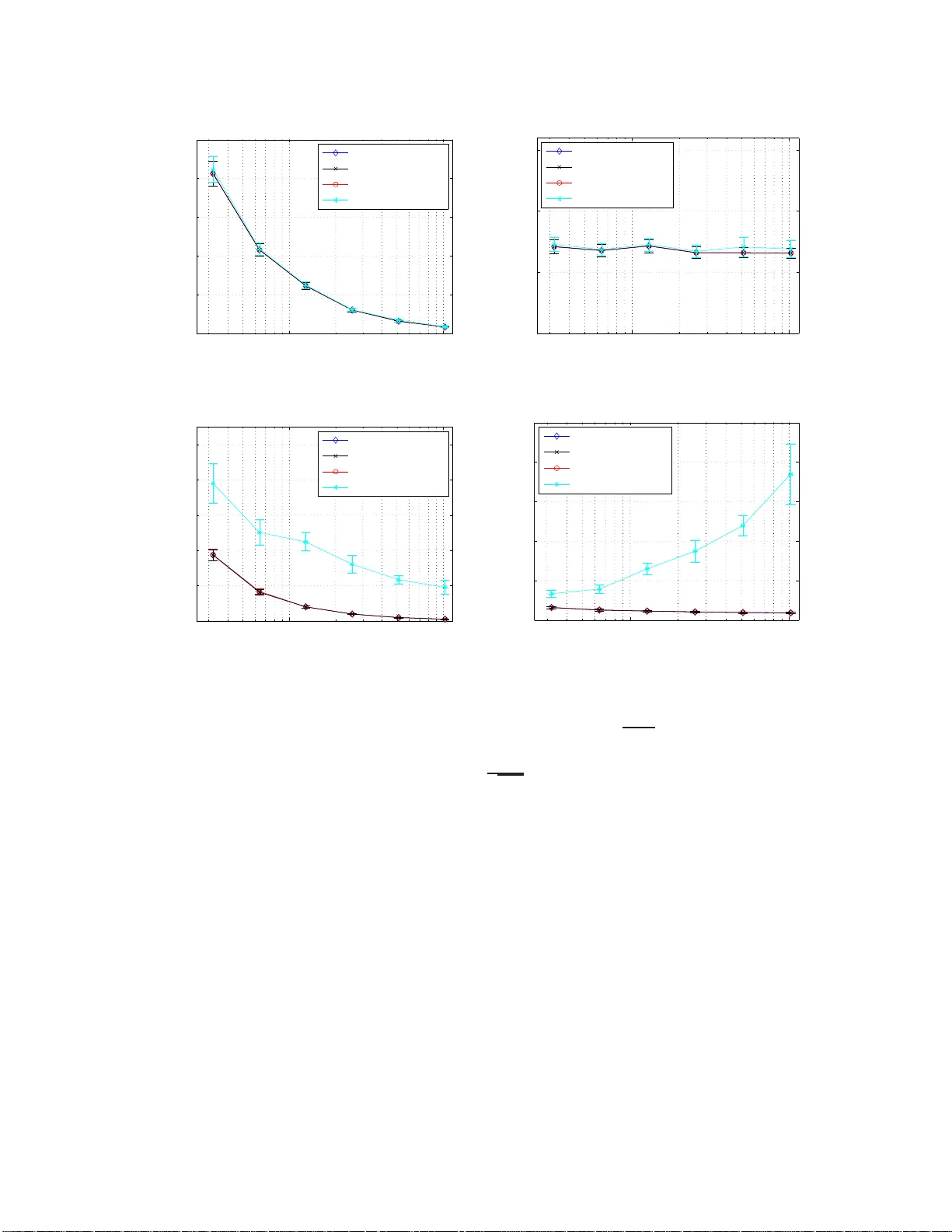
Randomized sk etc hes for k ernels: F ast and optimal non-parametric regress ion Y un Y ang 1 Mert Pilanci 1 Martin J. W ain wrigh t 1 , 2 Univ ersit y of California, Berk ele y 1 Departmen t of Electrical Engineering and Computer Science 2 Departmen t of Statistics Jan uary 27, 2015 Abstract Kernel ridge regr ession (KRR) is a standard metho d for p erfor ming non-para metric regres s ion o ver repro ducing kernel Hilbert spa ces. Given n samples, the time and space complexity of computing the KRR estimate s c a le as O ( n 3 ) a nd O ( n 2 ) r esp ectively , and so is prohibitive in many cases. W e prop ose appr oximations of KRR based on m -dimensional randomized sketc hes of the kernel matrix, and study how small the pr o jection dimension m can b e chosen while still pr eserving minimax o ptimalit y of the approximate KRR esti- mate. F or v arious classes o f randomized sketc hes, including thos e ba sed on Gauss ian and randomized Hadamard ma trices, we prove that it suffices to choo s e the sketc h dimension m prop o rtional to the statistical dimension (mo dulo log a rithmic factors). Thu s, we ob- tain fast a nd minimax optimal approximations to the K RR es timate for non-pa rametric regres s ion. 1 In tro duc tion The goal of non-parametric regression is to mak e predictions of a resp onse v ariable Y ∈ R based on observ in g a co v ariate v ector X ∈ X . In pr actice, w e are giv en a collection of n samples, sa y { ( x i , y i ) } n i =1 of co v ariate-resp onse pairs and our goal is to estimate the regression function f ∗ ( x ) = E [ Y | X = x ]. In the standard Gaussian mo del, it is assumed that the co v aria te-resp onse pairs are related via the mo del y i = f ∗ ( x i ) + σ w i , for i = 1 , . . . , n (1) where the sequence { w i } n i =1 consists of i.i.d. standard Gaussian v ariate s. I t is typical to assu me that the regression function f ∗ has s ome regularit y prop erties, and one w ay of enforcing su c h structure is to require f ∗ to b elong to a repro ducing ke rn el Hilb ert space, or RKHS for short [3, 28, 9]). Giv en such an assumption, it is natural to estimate f ∗ b y minimizing a com bination of the least-squares fit to the data and a p enalt y term inv olving the s q u ared Hilb ert norm, leading to an estimator known k ernel ridge r e gr ession , or KRR for short [10, 22]). F rom a statistica l p oint of view, th e b ehavior of KRR can b e c haracterized using existing r esults on M -estimation and empirical pro cesses (e.g. [13, 17, 26]). When the regularization parameter is set app ropriately , it is kn o wn to yield a function estimate w ith minim ax pred iction error for v arious classes of kernels. 1 Despite th ese attractiv e statistical pr op erties, the computational complexit y of compu ting the KRR estimate prev ent it from b eing routinely used in large-scale problems. More pr ecisely , in a standard implementat ion [21], the time complexity and space complexit y of KRR in a stand ard imp lemen tation scale as O ( n 3 ) and O ( n 2 ), resp ectiv ely , where n refers to the n umb er of samples. As a consequence, it b ecomes imp ortant to design metho ds to compu te appro ximate forms of the KRR estimate, while r etaining guaran tees of optimalit y in term s of statistical minimaxity . V arious authors hav e tak en differen t appr oac hes to this pr oblem. Zhang et al. [30] analyze a distributed implemen tation of K RR, in w hic h a set of t mac hines eac h compu te a separate estimate based on a random t -wa y p artition of the fu ll data set, and com bine it in to a global estimate b y a verag ing. Th is d ivide-and-conquer appr oac h has time complexit y and space complexity O ( n 3 /t 3 ) and O ( n 2 /t 2 ), resp ectiv ely . Zhang et al. [30 ] giv e conditions on the num b er of s plits t , as a f unction of the k ernel, under whic h minimax optimalit y of the resu lting estimator can b e guaran teed. More closely related to this pap er are metho ds that are based on f orm ing a lo w-rank appro ximation to the n -dimens ional k ernel matrix, suc h as the Nystr¨ om metho d s (e.g. [7, 8]). The time complexit y by usin g a lo w-rank appro ximation is either O ( nr 2 ) or O ( n 2 r ), d ep end in g on the sp eci fic approac h (excluding the time for factorizat ion), wh ere r is the maint ained rank, and th e sp ace complexit y is O ( nr ). Some recen t wo rk [4, 2] analyzes the tradeoff b etw een the rank r and the resulting statistical p erformance of the estimator, and we discus s this line of work at more length in Section 3.3. In this pap er, we consider approxi mations to KRR based on random pro jections, also kno wn as sk etc hes, of the data. Random p ro jections are a classical wa y of p erforming dimen- sionalit y reduction, and are widely us ed in many algorithmic con texts (e.g., see the b o ok [27 ] and references therein). Our pr op osal is to approximate n -d im en sional ke rn el matrix b y p ro- jecting its ro w and column sub spaces to a r andomly chosen m -d im en sional s ubspace with m ≪ n . By doing so, an app ro ximate f orm of the KRR estimate can b e obtained by s olving an m -dimensional quadratic program, which inv olv es time and sp ace complexit y O ( m 3 ) and O ( m 2 ). Computing the app ro ximate ke rn el matrix is a pr e-pro cessing s tep that has time complexit y O ( n 2 log( m )) f or s uitably chosen pro jections; this pre-pro cessing step is tr ivially parallelizable, meaning it can b e reduced to to O ( n 2 log( m ) /t ) by using t ≤ n clusters. Giv en s uc h an appr o ximation, we p ose the follo wing question: how s m all can the pro- jection dimension m b e c hosen wh ile still retaining minimax optimalit y of th e appro ximate KRR estimate? W e answer this question by connecting it to the statistic al dimension d n of the n -d im en sional ke rn el matrix, a quantit y that measures the effectiv e n umb er of degrees of freedom. (See Section 2.3 for a pr ecise defin ition.) F rom the results of earlier work on r andom pro jections for constr ained Least S quares estimators (e.g., see [18, 19]), it is natural to conjec- ture that it should b e p ossible to pro ject the k ernel matrix d o wn to the statistical dim en sion while preservin g minimax optimalit y of the resu lting estimator. The main con tribu tion of this p ap er is to confirm this conjecture f or several classes of random pro jection matrices. The remainder of this pap er is organized as follo ws. Section 2 is devo ted to furth er bac kground on n on-parametric regression, repro du cing k ernel Hilb ert spaces and asso ciated measures of complexit y , as we ll as the notion of statistical dimen s ion of a kernel. In S ection 3, w e turn to statemen ts of our main resu lts. Th eorem 2 pro vides a general sufficien t condition on a rand om sketc h f or th e asso ciated appr o ximate form of KRR to ac hieve the minimax risk. In Corollary 1, we derive s ome consequ ences of this general result for particular classes of random sketc h matrices, and confirm these theoretical pr edictions with some simulat ions. W e also compare at m ore length to metho ds based on th e Nystr¨ om approximati on in Section 3.3. Section 4 is devote d to the pro ofs of our main results, with the pro ofs of more tec hnical results deferred to th e app en dices. W e conclude with a d iscussion in Section 5. 2 2 Problem form ulation and bac kground W e b egi n by introdu cing some bac kground on non p arametric regression and repro du cing k ernel Hilb ert spaces, b efore form ulating the problem discussed in this pap er. 2.1 Regression in repro ducing k ernel Hilb ert spaces Giv en n samples { ( x i , y i ) } n i =1 from th e non-p arametric regression m o del (1), our goal is to estimate th e unknown regression fu nction f ∗ . Th e qualit y of an estimate b f can b e measured in d ifferen t wa ys: in this pap er, we fo cus on the s q u ared L 2 ( P n ) error k b f − f ∗ k 2 n : = 1 n n X i =1  b f ( x i ) − f ∗ ( x i )  2 . (2) Naturally , the difficult y of non-parametric r egression is con trolled by the structure in the function f ∗ , and on e wa y of mo deling such str u cture is within the framew ork of a repr o ducing k ernel Hilb ert space (or RKHS for s h ort). Here we pro vide a v ery br ief in tro d uction r eferring the reader to the b o oks [6, 9, 28] f or more details and bac kground. Giv en a space X endo w ed with a probability distribution P , the space L 2 ( P ) consists of all fu nctions that are s quare-in tegrable w ith resp ect to P . In abstract terms, a sp ace H ⊂ L 2 ( P ) is an RKHS if for eac h x ∈ X , th e ev aluatio n function f 7→ f ( x ) is a b ound ed linear fun ctional. In m ore concrete terms, any RK HS is generated by a p ositiv e semidefinite (PSD) k ernel function in the f ollo wing wa y . A PSD k ernel f u nction is a symmetric fun ction K : X × X → R such that, f or any p ositiv e inte ger N , collectio ns of p oin ts { v 1 , . . . , v N } and w eigh t v ector ω ∈ R N , the sum P N i,j =1 ω i ω j K ( v i , v j ) is non-negativ e. S upp ose moreo ve r that for eac h fi xed v ∈ X , the f u nction u 7→ K ( u, v ) b elongs to L 2 ( P ). W e can then consider the v ector space of all fu nctions g : X → R of the form g ( · ) = N X i =1 ω i K ( · , v i ) for some intege r N , p oin ts { v 1 , . . . , v N } ⊂ X and weig ht vecto r w ∈ R N . By taking the closure of all suc h linear com bin ations, it can b e shown [3] that w e generate an RKHS, and one that is uniqu ely asso ciated with the k ernel K . W e p ro vide some examples of v arious kernels and the asso ciated function classes in Section 2.3 to follo w. 2.2 Kernel ridge regr ession and its sketc hed form Giv en th e dataset { ( x i , y i ) } n i =1 , a natur al metho d for estimating unk n o wn fun ction f ∗ ∈ H is kno wn as k ernel ridge regression (KRR): it is based on the conv ex p rogram f † : = arg min f ∈H n 1 2 n n X i =1  y i − f ( x i )  2 + λ n k f k 2 H o , (3) where λ n is a regularization parameter. As stated, this optimization problem can b e infin ite-dimensional in nature, sin ce it take s place o v er the Hilb ert space. Ho w ev er, as a straigh tforw ard consequ ence of the repr esenter theorem [12], the solution to this optimization problem can b e obtained by s olving the n - dimensional conv ex pr ogram. In particular, let us defi n e the e mpiric al kernel matrix , namely 3 the n -dimensional symmetric matrix K with en tries K ij = n − 1 K ( x i , x j ). Here w e adopt the n − 1 scaling for later theoretical con v enience. In terms of this matrix, the KRR estimate can b e obtained b y first solving the quadratic program ω † = arg min ω ∈ R n n 1 2 ω T K 2 ω − ω T K y √ n + λ n ω T K ω o , (4a) and then outpu tting the fun ction f † ( · ) = 1 √ n n X i =1 ω † i K ( · , x i ) . (4b) In principle, the original K RR optimization problem (4a) is s im p le to s olv e: it is an n dimensional quadr atic program, and can b e solv ed exactly usin g O ( n 3 ) via a QR decomp o- sition. Ho we ver, in man y applications, the num b er of samples m ay b e large, so that th is t yp e of cubic s caling is p rohibitiv e. In addition, the n -dimens ional k ernel m atrix K is d ense in general, and so requires storage of ord er n 2 n umb ers, which can also b e problematic in practice. In this pap er, w e consider an appr oximati on based on limiting the original parameter ω ∈ R n to an m -dimensional sub space of R n , where m ≪ n is the pr oje ctio n dimension . W e define this app r o ximation via a sketc h matrix S ∈ R m × n , such that the m -d imensional subspace is generated by the ro w span of S . More precisely , the sketche d kernel ridge r e gr ession estimate is given by first solving b α = arg min θ ∈ R m n 1 2 α T ( S K )( K S T ) α − α T S K y √ n + λ n α T S K S T α o , (5a) and then outpu tting the fun ction b f ( · ) : = 1 √ n n X i =1 ( S T b α ) i K ( · , x i ) . (5b) Note that the sket ched pr ogram (5a) is a qu adratic pr ogram in m dimensions: it tak es as in- put the m -dimensional matrices ( S K 2 S T , S K S T ) and the m -dimensional v ector S K y . Con- sequen tly , it can b e solve d efficien tly via QR decomp osition w ith computational complexit y O ( m 3 ). Moreo v er, the computation of the ske tc hed kernel matrix S K = [ S K 1 , . . . , S K n ] in the input can b e parallellized across its columns. In this pap er, w e analyze v arious f orms of r andom sk etc h matrices S . Let us consider a few of them here. Sub-Gaussian sketc hes: W e sa y the row s i of the ske tc h mat rix is zero-mean 1-sub- Gaussian if for an y fix ed un it v ector u ∈ S n − 1 , we hav e P  |h u, s i i ≥ t |  ≤ 2 e − nδ 2 2 for all δ ≥ 0. Man y standard c hoices of sket ch matrices hav e i.i.d. 1-sub-Gaussian ro ws in th is sense; exam- ples include matrices with i.i.d. Gaussian entries, i.i.d. Bernou lli entries, or random matrices with in d ep endent r o ws d ra wn uniformly from a rescaled sph ere. F or con venience, the sub- Gaussian sk etc h matrices considered in this p ap er are all rescaled so that their rows h a v e the co v aria nce matrix 1 √ m I n × n . 4 Randomized orthogonal system (R OS) sk etc hes: This class of sketc hes are b ased on randomly sampling and rescaling the r o ws of a fi xed orth onormal matrix H ∈ R n × n . Examples of suc h matrices include the discrete F ourier transform (DFT) matrix, and the Hadamard matrix. More sp ecifically , a ROS sk etc h m atrix S ∈ R m × n is form ed w ith i.i.d. ro ws of th e form s i = r n m RH T p i , for i = 1 , . . . , m, where R is a random diagonal matrix whose entries are i.i.d. Rademac her v ariables and { p 1 , . . . , p m } is a r andom subset of m ro ws s ampled uniformly f rom the n × n id en tit y matrix without r eplacemen t. An adv an tage of using R OS s k etc hes is that for suitably c hosen or- thonormal m atrices, including the DFT and Hadamard cases among others, a matrix-v ector pro du ct (say of the form S u for some v ector u ∈ R n ) can b e computed in O ( n log m ) time, as opp osed to O ( nm ) time required for the same op eration w ith generic dens e sk etc hes. F or instance, see Ailon and Lib erty [1 ] and [18] for further d etails. Throu gh ou t this pap er, w e fo cus on ROS sketc hes based on orthonormal matrices H with un iformly b ounded en tries, meaning that | H ij | ≤ c √ n for all en tries ( i, j ). This entrywise b ound is s atisfied by Hadamard and DFT matrices, among others. Sub-sampling sketc hes: This class of sketc hes are ev en simp ler, based on sub -sampling th e ro ws of the ident ity matrix without replacemen t. In particular, the sket ch m atrix S ∈ R m × n has ro ws of the form s i = p n m p i , where the vect ors { p 1 , . . . , p m } are dr a wn uniform ly at random without r ep lacemen t from the n -dimensional id en tit y matrix. It can b e understo o d as related to a R OS sk etc h, based on the identit y m atrix as an orthon orm al matrix, and not using the Rademac her randomization nor satisfying the en trywise b ound. I n App endix A, w e sho w that the ske tc hed KRR estimate (5a) based on a su b-sampling sket ch matrix is equiv ale nt to the Nystr¨ om appr o ximation. 2.3 Kernel complexit y measures and statistical guaran tees So as to set the stage for later results, let us characte rize an appr opriate c hoice of the regu- larizatio n parameter λ , and the resu lting b ound on the prediction err or k f † − f ∗ k n . Recall the empir ical k ernel matrix K d efined in the previous section: s in ce it is symmetric and p os- itiv e definite, it has an eigendecomp osition of the form K = U D U T , wh ere U ∈ R n × n is an orthonormal matrix, and D ∈ R n × n is diagonal with elemen ts b µ 1 ≥ b µ 2 ≥ . . . ≥ b µ n ≥ 0. Using these eigen v a lues, consider the ke rnel c omplexity fu nction b R ( δ ) = v u u t 1 n n X j =1 min { δ 2 , b µ j } , (6) corresp ondin g to a rescaled su m of the eigen v alues, trun cated at lev el δ 2 . This f unction arises via analysis of the lo ca l R ad emacher complexit y of the k ernel class (e.g., [5 , 13, 17, 20]). F or a giv en k ernel matrix and noise v ariance σ > 0, the c ritic al r adius is defined to b e the smallest p ositiv e solution δ n > 0 to the inequalit y b R ( δ ) δ ≤ δ σ . (7) Note that the existence and uniqueness of this critical radiu s is guarante ed for any kernel class [5 ]. 5 Bounds on ordinary KRR: The significance of the critical radiu s is th at it can b e used to sp ecify b ounds on th e pr ediction error in k ernel rid ge r egression. More precisely su pp ose that we compute the KRR estimate (3) with any regularization parameter λ ≥ 2 δ 2 n . Th en with p robabilit y at least 1 − c 1 e − c 2 nδ 2 n , w e are guarantee d that k f † − f ∗ k 2 n ≤ c u  λ n + δ 2 n  , (8) where c u > 0 is a unive rs al constant (in d ep end ent of n , σ and the k ernel). This kno wn result follo ws from standard tec hniqu es in emp ir ical pr o cess theory (e.g., [26, 5]); we also note that it can b e obtained as a corollary of our more general theorem on sk etc hed KRR estimates to follo w (viz. Theorem 2). T o illustrate, let us consider a few examples of repro ducing k ernel Hilb ert spaces, and compute the critical radius in different cases. In working through these examples, so as to determine explicit rates, w e assume that the design p oint s { x i } n i =1 are s amp led i.i.d. from some u nderlying distribution P , and we make use of the u seful fact that, u p to constan t factors, w e can alwa ys w ork with the p opulation-lev el kernel complexit y function R ( δ ) = v u u t 1 n ∞ X j =1 min { δ 2 , µ j } , (9) where { µ j } ∞ j =1 are the eigen v alues of the ke rn el integ ral op erator (assum ed to b e u niformly b ound ed). T his equ iv al ence follo ws from standard r esults on the p opulation and empirical Rademac her complexities [17, 5]. Example 1 (Polynomia l k ern el) . F or s ome intege r D ≥ 1, consider the kernel fu nction on [0 , 1] × [0 , 1] giv en by K poly ( u, v ) =  1 + h u, v i  D . F or D = 1, it generates the class of all linear functions of the form f ( x ) = a 0 + a 1 x for some scalars ( a 0 , a 1 ), and corresp onds to a linear k ernel. More generally , for larger integ ers D , it generates the class of all p olynomial functions of d egree at most D —that is, functions of the form f ( x ) = P D j =0 a j x j . Let u s n o w compute a b ound on the critical r adius δ n . It is straightfo rward to sho w that the p olynomial k ernel is of fin ite rank at most D + 1, meaning that the k ern el matrix K alw a ys has at most min { D + 1 , n } non-zero eigen v alues. Consequent ly , as long n > D + 1, there is a unive rsal constan t c such that b R ( δ ) ≤ c r D + 1 n δ , whic h implies that δ 2 n - σ 2 D +1 n . Consequently , we conclude that the KRR estimate satisifes the b ound k b f − f ∗ k 2 n - σ 2 D +1 n with high p robabilit y . Note that this b ound is in tuitiv e, since a p olynomial of degree D h as D + 1 free parameters. Example 2 (Gaussian k ernel) . The Gaussian k ernel with bandwidth h > 0 tak es the f orm K gau ( u, v ) = e − 1 2 h 2 ( u − v ) 2 . When defined with resp ect to Leb esgue measure on the real line, the eigen v alues of the ke rn el integ ral op erator scale as µ j ≍ exp ( − π h 2 j 2 ) as j → ∞ . Ba sed on this fact, it can b e shown that the critical radiu s scales as δ 2 n ≍ σ 2 n q log  n σ 2  . T h us , ev en though the Gaussian k ernel is non-parametric (since it cannot b e sp ec ified by a fixed n umb er of parametrers), it is still a r elativ ely small function class. 6 Example 3 (First-order S ob olev space) . As a final example, consider the ke rn el d efi ned on the unit s q u are [0 , 1] × [0 , 1] giv en b y K sob ( u, v ) = min { u, v } . It generates the function class H 1 [0 , 1] = n f : [0 , 1] → R | f (0) = 0 , and f is abs. cts. with R 1 0 [ f ′ ( x )] 2 dx < ∞  , (10) a class that con tains all Lipschitz f u nctions on the u nit in terv al [0 , 1]. Roughly sp eaking, we can think of the fir st-order Sob olev class as functions th at are almost eve ryw h ere differentiable with deriv ativ e in L 2 [0 , 1]. Note that this is a m uch larger k ern el class than the Gaussian k ernel class. The fi rst-order Sob olev space can b e generalized to h igher ord er S ob olev s paces, in wh ic h functions ha v e add itional smo othn ess. See the b ook [9] for fu rther details on these and other r epro du cing k ernel Hilb ert spaces. If the kernel integral op er ator is defined with resp ect to Leb esgue measure on the unit in terv al, then the p opu lation lev el eigen v alues are giv en by µ j =  2 (2 j − 1) 2 π  2 for j = 1 , 2 , . . . . Giv en this relation, some calculation sh ows that the critical r adius s cales as δ 2 n ≍  σ 2 n  2 / 3 . This is the familiar minimax risk f or estimating Lipschitz fun ctions in one dimension [23]. Lo wer b ounds for non-parametric regression: F or futur e reference, it is also con venien t to provide a lo wer b ound on the prediction err or ac hiev able b y any estimator . In order to do so, we fi r st define the statistic a l dimension of the k ernel as d n : = arg min j =1 ,...,n  b µ j ≤ δ 2 n } , (11) and d n = n if no su c h in dex j exists. By definition, we are guaran teed th at b µ j > δ 2 n for all j ∈ { 1 , 2 , . . . , d n } . I n terms of this statistica l dimension, w e hav e b R ( δ n ) = h d n n δ 2 n + 1 n n X j = d n +1 b µ j i 1 / 2 , sho wing that the s tatistical dim en sion control s a type of bias-v ariance tradeoff. It is reasonable to exp ect that the critical rate δ n should b e related to the s tatistical dimension as δ 2 n ≍ σ 2 d n n . Th is scaling relation holds wheneve r the tail sum satisfies a b ound of the form P n j = d n +1 b µ j - d n δ 2 n . Although it is p ossible to construct pathological examples in whic h this scaling relation do es n ot hold, it is tru e for m ost kernels of interest, in clud ing all examples considered in this pap er. F or any suc h regular ke rn el, th e critical radius pro vides a fundamental lo we r b ound on the p erformance of any estimator , as summ arized in the follo wing theorem: Theorem 1 (Critical r adius and m inimax r isk) . Given n i.i.d. samples { ( y i , x i ) } n i =1 fr om the standar d non-p ar ametric r e gr ession mo d el over any r e gular k ernel class, any estimator e f has pr e diction e rr or lower b ounde d as sup k f ∗ k H ≤ 1 E k e f − f ∗ k 2 n ≥ c ℓ δ 2 n , (12) wher e c ℓ > 0 is a numeric al c onstant, and δ n is the critic al r adius (7) . The p ro of of this claim, pr o vided in App end ix B.1, is based on a standard applicaton of F ano’s inequalit y , com bin ed with a ran d om pac king argument. It establishes that the critical r adius is a fund amen tal quan tit y , corresp ondin g to the app ropriate b enc hmark to which ske tc hed k ernel regression estimates should b e compared. 7 3 Main r esults and their consequences W e no w turn to statement s of our main theorems on kernel sket ching, as we ll as a discussion of some of their consequen ces. W e fir st introdu ce the n otion of a K -satisfiable sk etc h matrix, and then sho w (in T h eorem 2) that any sket ched KRR estimate based on a K -satisfiable ske tc h also ac hieves the minimax risk. W e illustrate this ac h iev able result with sev eral corollaries for differen t t yp es of randomized sk etc hes. F o r Gaussian and ROS ske tc hes, w e show that c ho osing the sk etc h dimens ion pr op ortional to the s tatistical dimens ion of the kernel (with additional log factors in the R OS case) is sufficient to guaran tee that the r esulting sk etc h will b e K - satisfiable with high pr obabilit y . In addition, w e illustrate the sh arpness of our theoretical predictions via some exp erim ental simulat ions. 3.1 General conditions for sk etched k ernel optimalit y Recall the defin ition (11) of the statistical dimension d n , and consid er the eigendecomp osition K = U D U T of the k ernel matrix, where U ∈ R n × n is an orthonormal m atrix of eigen v ectors, and D = diag { b µ 1 , . . . , b µ n } is a diagonal m atrix of eigen v alues. Let U 1 ∈ R n × d n denote the left blo c k of U , and similarly , U 2 ∈ R n × ( n − d n ) denote th e righ t blo ck. Note that the columns of the left b lo c k U 1 corresp ond to the eigen v ectors of K asso cia ted with the leading d n eigen v alues, whereas th e columns of the righ t blo ck U 2 corresp ond to th e eigen ve ctors asso ciated with the remaining n − d n smallest eigen v alues. Int uitively , a sket ch matrix S ∈ R m × n is “go o d ” if the sub-matrix S U 1 ∈ R m × d n is relativ ely close to an isometry , whereas th e sub -matrix S U 2 ∈ R m × ( n − d n ) has a relativ ely small op erator norm. This in tuition can b e formalized in the follo wing w a y . F or a giv en kernel matrix K , a sk etc h m atrix S is said to b e K -satisfia ble if there is a universal constan t c such that | | | ( S U 1 ) T S U 1 − I d n | | | op ≤ 1 / 2 , and | | | S U 2 D 1 / 2 2 | | | op ≤ c δ n , (13) where D 2 = diag { b µ d n +1 , . . . , b µ n } . Giv en this defin ition, the follo wing theorem sh o ws that any ske tc hed KRR estimate based on a K -satisfiable matrix ac h iev es the minimax r isk (with high p r obabilit y o v er th e noise in the observ ation mo del): Theorem 2 (Upp er b ound) . Given n i.i.d. samples { ( y i , x i ) } n i =1 fr om the standar d non- p ar ametric r e gr ession mo del, c onsider the sketche d KRR pr oblem (5a) b ase d on a K -satisfiable sketch matrix S . Then any for λ n ≥ 2 δ 2 n , the sketche d r e gr ession estimate b f fr om e quation (5b) satisfies the b ound k b f − f ∗ k 2 n ≤ c u  λ n + δ 2 n  with pr ob ability gr e ater than 1 − c 1 e − c 2 nδ 2 n . W e emp hasize that in the case of fixed design regression and for a fixed ske tc h matrix, the K -satisfiable condition on the sk etc h matrix S is a determin istic s tatemen t: apart from the sket ch matrix, it only dep end s on the prop erties of the kernel function K and design v ariables { x i } n i =1 . Thus, wh en us in g ran d omized sketc hes, the algorithmic randomness can b e completely decoupled fr om the rand omness in the noisy obser v ation mo del (1 ). 8 Pro of intuition: The pro of of Th eorem 2 is give n in S ection 4.1. A t a high-lev el, it is based on an upp er b oun d on the prediction error k b f − f ∗ k 2 n that in vo lves t wo sources of error: the appr oximation e rr or asso ciated with solving a zero-noise v ersion of the KRR pr ob lem in the p ro jected m -dimen s ional space, and the estimation err or b etw een the noiseless and noisy v ersions of the pro jected pr oblem. In more d etail, letting z ∗ : = { f ∗ ( x 1 ) , . . . , f ∗ ( x n ) } denote the v ector of fu nction ev aluations defined b y f ∗ , consider the quad r atic program α † : = arg min α ∈ R m n 1 2 n k z ∗ − √ nK S T α k 2 2 + λ n k √ K S T α k 2 2 o , (14) as well as the asso ciated fitted fu nction f † = 1 √ n P n i =1 α † i K ( · , x i ). The vecto r α † ∈ R m is the solution of the sk etc hed problem in the case of zero noise, whereas the fitted function f † corresp onds to the b est p enalized appro ximation of f ∗ within the range space of S T . Giv en this definition, w e then ha v e th e elemen tary inequ ality 1 2 k b f − f ∗ k 2 n ≤ k f † − f ∗ k 2 n | {z } Appro ximation error + k f † − b f k 2 n | {z } Estimation err or . (15) F or a fixed sk etc h matrix, the approximat ion error term is determin istic: it corresp onds to the error indu ced by app r o ximating f ∗ o v er the range sp ace of S T . On the other hand , the estimation error d ep ends b oth on the ske tc h matrix and the observ ation noise. In S ection 4.1, w e state and pr o v e tw o lemmas that con trol the appro ximation and error terms r esp ectiv ely . As a corollary , Th eorem 2 implies the stated u p p er b ound (8) on the prediction err or of the original (unsket ched) KRR estimate (3). Ind eed, th is estimator can b e obtained using the “sk etc h matrix” S = I n × n , w h ic h is easily seen to b e K -satisfiable. In practice, h o w eve r, w e are inte rested in m × n sketc h matrices with m ≪ n , so as to ac hieve computational sa vings. In particular, a n atural conjecture is that it should b e p ossib le to efficien tly generate K -sat isfiab le sk etc h matrices w ith the pro jection d imension m p rop ortional to the statistical d im en sion d n of the k ernel. Of course, one suc h K -sat isfiable matrix is giv en by S = U T 1 ∈ R d n × n , bu t it is not easy to generate, sin ce it requires computing the eigendecomp osition of K . Nonetheless, as w e now sho w, there are v arious randomized constructions that lead to K -sa tisfiable sketc h matrices with high pr obabilit y . 3.2 Corollaries for randomized sk etches When com bined with add itional probabilistic analysis, Th eorem 2 implies th at v arious forms of r an d omized ske tc hes ac h iev e the minimax r isk using a sk etc h dimension prop ortional to the statistica l d imension d n . Here we analyze the Gaussian and ROS families of rand om s ketc hes, as pr eviously defi n ed in Section 2.2. Throughout our an alysis, we require that the sk etc h dimension satisfies a low er obun d of the form m ≥ ( c d n for Gaussian sketc hes, and c d n log 4 ( n ) for R OS sk etc hes, (16a) where d n is the statistic al dimension as pr eviously d efined in equation (11 ). Here it should b e u ndersto o d that the constant c can b e chosen sufficiently large (but fi n ite). In addition, for the p u rp oses of stating high probabilit y results, we defin e the f unction φ ( m, d n , n ) : =    c 1 e − c 2 m for Gaussian ske tc hes, and c 1  e − c 2 m d n log 2 ( n ) + e − c 2 d n log 2 ( n )  for ROS sketc hes , (16b) 9 where c 1 , c 2 are universal constants. With this notation, the follo w ing r esult pro vides a h igh probabilit y guarant ee for b oth Gaussian and ROS sk etc hes: Corollary 1 (Guaran tees for Gaussian and ROS sketc hes) . Given n i.i . d. samples { ( y i , x i ) } n i =1 fr om the standar d non-p ar ametric r e gr ession mo del (1) , c onsider the sketche d KRR pr ob- lem (5a) b ase d on a sketch dimension m satisfying the lower b ound (16a) . Then ther e is a universal c onstant c ′ u such that for any λ n ≥ 2 δ 2 n , the sketche d r e gr e ssion estimate (5b) satisfies the b ound k b f − f ∗ k 2 n ≤ c ′ u  λ n + δ 2 n  with pr ob ability gr e ater than 1 − φ ( m, d n , n ) − c 3 e − c 4 nδ 2 n . In order to illus tr ate Corollary 1, let us r eturn to the three examples previously discussed in Section 2.3. T o b e concrete, we d er ive the consequences for Gaussian sk etc hes, noting that R OS sk etc hes incur only an additional log 4 ( n ) ov erhead. • for the D th -order p olynomial k ernel from Example 1, the statistica l dimension d n for an y sample size n is at most D + 1, so that a s k etc h size of order D + 1 is su fficien t. T his is a v ery sp eci al case, since the k ernel is finite rank and so the r equired sketc h dimension has no d ep endence on the sample size. • for the Gaussian kernel from Examp le 2, th e statistical d imension satisfies th e scaling d n ≍ √ log n , so that it s uffices to tak e a sk etc h dimension scaling logarithmically with the sample size. • for the first-order Sob olev k ernel fr om Example 3 , the statistica l dimension scales as d n ≍ n 1 / 3 , so that a sk etc h d imension scaling as the cub e ro ot of the sample size is required. In order to illustrate these theoretical predictions, we p erformed some simulations. Be- ginning with the Sob olev k ernel K sob ( u, v ) = min { u, v } on the unit square, as introdu ced in Example 3, we generated n i.i.d. samp les from the mo d el (1) with noise standard d eviation σ = 1, the unknown r egression function f ∗ ( x ) = | x + 0 . 5 | − 0 . 5 , (17) and uniformly sp aced design p oin ts x i = i n for i = 1 , . . . , n . By constru ction, the function f ∗ b elongs to the first-order Sob ole v space with k f ∗ k H = 1. As suggested by our theory for the Sob olev k ernel, we set the p ro jection d imension m = ⌈ n 1 / 3 ⌉ , and then s olv ed the ske tc hed ver- sion of k ernel r idge regression, for b oth Gauss ian ske tc hes and R OS ske tc hes based on the fast Hadamard transform . W e p erformed simulat ions for n in th e set { 32 , 64 , 128 , 256 , 512 , 1024 } so as to stud y scaling with the s amp le s ize. As noted ab ov e, our theory predicts that the squared p rediction loss k b f − f ∗ k 2 n should tend to zero at the same rate n − 2 / 3 as that of the unsket ched estimator f † . Figure 1 confir ms this theoretical prediction. In panel (a), we plot the squared p rediction error v ersus the sample size, showing that all three curv es (original, Gaussian ske tc h and R OS sketc h) tend to zero. Pa nel (b) plots th e r esc ale d p rediction error n 2 / 3 k b f − f ∗ k 2 n v ersus the sample size, w ith th e relativ e flatness of these cu r v es confirming the n − 2 / 3 deca y predicted by our theory . In our second exp eriment, w e rep eate d the same set of simulati ons this time for the Gaus- sian k ern el K gau ( u, v ) = e − 1 2 h 2 ( u − v ) 2 with band width h = 0 . 25, and the function f ∗ ( x ) = − 1 + 2 x 2 . 10 10 2 10 3 0 0.01 0.02 0.03 0.04 Sample size Squared prediction loss Pred. error for Sobolev kernel Original KRR Gaussian sketch ROS sketch 10 2 10 3 0 0.1 0.2 0.3 0.4 0.5 0.6 Sample size Rescaled prediction loss Pred. error for Sobolev kernel Original KRR Gaussian sketch ROS sketch (a) (b) Figure 1. Prediction erro r versus sample size for or iginal KRR, Gaussian sketc h, and ROS sketc hes for the Sob o lev one kernel for the function f ∗ ( x ) = | x + 0 . 5 | − 0 . 5. In all cases, each po int cor resp onds to the average of 100 trials , with standa rd errors also shown. (a) Squared prediction err or k b f − f ∗ k 2 n versus the sample size n ∈ { 32 , 6 4 , 128 , 2 56 , 1024 } for pro jection dimension m = ⌈ n 1 / 3 ⌉ . (b) Rescaled prediction er ror n 2 / 3 k b f − f ∗ k 2 n versus the sample s ize. In this case, as suggested by our theory , we c ho ose the ske tc h dimens ion m = ⌈ 1 . 25 √ log n ⌉ . Figure 2 sh o ws the same t yp es of plots with the prediction error. In this case, w e exp ect that the squ ared prediction err or w ill deca y at the rate √ log n n . Th is prediction is confirmed by the plot in p anel (b), sh owing that the rescaled error n √ log n k b f − f ∗ k 2 n , when plotted v ersus the sample size, remains relativ ely constant ov er a wide range. 3.3 Comparison with N ystr¨ om- based approac hes It is interesting to compare th e conv ergence rate and compu tational complexit y of our m eth- o ds with guarantee s based on the Nystr¨ om approximati on. As shown in App endix A, this Nystr¨ om appr o ximation approac h can b e under s to o d as a particular form of our sketc hed estimate, one in which the sk etc h corresp onds to a random row-sa mp ling matrix. Bac h [4] analyzed the prediction error of th e Nystr¨ om approxima tion to K R R based on uniformly samp ling a su bset of p -columns of the kernel matrix K , leading to an o ve rall com- putational complexit y of O ( np 2 ). In order for the app r o ximation to matc h the p erformance of KRR, the num b er of sampled columns must b e lo w er b ound ed as p % n k diag( K ( K + λ n I ) − 1 ) k ∞ log n, a quan tit y whic h can b e subs tan tially larger than the statistical dimens ion required by our metho ds. Moreo ver, as shown in the follo win g example, there are many classes of k ernel matrices for w hic h the p erformance of the Nys tr ¨ om approximati on will b e p oor. Example 4 (F ailure of Nystr¨ om appr o ximation) . Giv en a ske tc h d imension m ≤ n log 2, consider an empirical kernel matrix K that h as a blo c k diagonal form diag( K 1 , K 2 ), w here K 1 ∈ R ( n − k ) × ( n − k ) and K 2 ∈ R k × k for an y integ er k ≤ n m log 2. Then the pr obabilit y of n ot sampling an y of the last k column s/ro ws is at least 1 − (1 − k /n ) m ≥ 1 − e − k m/n ≥ 1 / 2. This means th at with probabilit y at least 1 / 2, the su b-sampling sketc h matrix can b e expressed as 11 10 2 10 3 0 0.005 0.01 0.015 0.02 0.025 0.03 Sample size Squared prediction loss Pred. error for Gaussian kernel Original KRR Gaussian sketch ROS sketch 10 2 10 3 0 0.1 0.2 0.3 0.4 0.5 0.6 Sample size Rescaled prediction loss Pred. error for Gaussian kernel Original KRR Gaussian sketch ROS sketch (a) (b) Figure 2. Prediction erro r versus sample size for or iginal KRR, Gaussian sketc h, and ROS sketc hes for the Gaussian kernel with the function f ∗ ( x ) = − 1 + 2 x 2 . In a ll cases, each po int cor resp onds to the average of 100 trials , with standa rd errors also shown. (a) Squared prediction err or k b f − f ∗ k 2 n versus the sample size n ∈ { 32 , 6 4 , 128 , 2 56 , 1024 } for pro jection dimension m = ⌈ 1 . 25 √ log n ⌉ . (b) Rescaled prediction erro r n √ log n k b f − f ∗ k 2 n versus the sample size. S = ( S 1 , 0), wh ere S 1 ∈ R m × ( n − k ) . Und er such an ev ent, the sketc hed K RR (5a) tak es on a degenerate form, n amely b α = arg min θ ∈ R m n 1 2 α T S 1 K 2 1 S T 1 α − α T S 1 K 1 y 1 √ n + λ n α T S 1 K 1 S T 1 α o , and ob jectiv e that dep ends only on the fir st n − k observ ations. Since the v alues of the last k observ ations can b e arbitrary , this d egeneracy has th e p otenti al to lead to sub stan tial appro ximation error. The pr evious example suggests th at the Nystr¨ om ap p ro ximation is likel y to b e very sensi- tiv e to n on-inhomogeneit y in the samp ling of co v ariates. In order to explore this conjecture, w e p erform ed some additional sim ulations, this time comparing b oth Gaussian and R OS sk etc hes with the un iform Nystr¨ om app ro ximation sket ch. Returnin g again to the Gauss ian k ernel K gau ( u, v ) = e − 1 2 h 2 ( u − v ) 2 with band width h = 0 . 25, and the fun ction f ∗ ( x ) = − 1 + 2 x 2 , w e fir st generated n i.i.d. samples that were unif orm on the un it in terv al [0 , 1]. W e then im- plemen ted sketc hes of v arious t yp es (Gaussian, R OS or Nystr¨ om) u sing a sketc h d im en sion m = ⌈ 4 √ log n ⌉ . As sh o wn in the top ro w (panels (a) and (b)) of Figur e 3, all three sk etc h t yp es p erform ve ry we ll for this regular design, with p rediction err or that is essentia lly indis- tiguishable from the original K RR estimate. Keeping the same k ern el and fun ction, we then considered an ir regular form of design, namely with k = ⌈ √ n ⌉ samples p erturb ed as follo ws : x i ∼ ( Unif [0 , 1 / 2] if i = 1 , . . . , n − k 1 + z i for i = k + 1 , . . . , n where eac h z i ∼ N (0 , 1 /n ). The p erformance of th e sketc hed estimators in this case are sh o wn in the b ottom ro w (panels (c) and (d)) of Figure 3. As b efore, b oth th e Gaussian and ROS sk etc hes trac k the p erformance of the original KRR estimate v ery closely; in con trast, th e 12 10 2 10 3 0 0.01 0.02 0.03 0.04 0.05 Sample size Squared prediction loss Gaussian kernel; regular design Original KRR Gaussian sketch ROS sketch Nystrom 10 2 10 3 0 0.5 1 1.5 Sample size Rescaled prediction loss Gaussian kernel; regular design Original KRR Gaussian sketch ROS sketch Nystrom (a) (b) 10 2 10 3 0 0.02 0.04 0.06 0.08 0.1 Sample size Squared prediction loss Gaussian kernel; irregular design Original KRR Gaussian sketch ROS sketch Nystrom 10 2 10 3 0 2 4 6 8 10 Sample size Rescaled prediction loss Gaussian kernel; irregular design Original KRR Gaussian sketch ROS sketch Nystrom (c) (d) Figure 3. Predictio n er ror versus sample size for orig inal KRR, Gauss ian sketc h, ROS sketc h and Nys tr¨ om a pproximation. Left panels (a) and (c) shows k b f − f ∗ k 2 n versus the s a mple size n ∈ { 3 2 , 64 , 12 8 , 256 , 1024 } for pro jection dimension m = ⌈ 4 √ log n ⌉ . In all cases, each po int co rresp onds to the average of 1 00 tria ls, with standard er rors also shown. Rig ht panels (b) and (d) show the rescaled predictio n erro r n √ log n k b f − f ∗ k 2 n versus the s ample size. T op row corr e s po nd to c ov a riates a rrange d uniformly on the unit interv al, wherea s b ottom row corres p o nds to a n irreg ular de s ign (see text for deta ils). Nystr¨ om appr o ximation b ehav es ve ry p o orly for this r egression problem, consisten t with the in tuition suggested b y the preceding example. As is kno wn f rom general theory on the Nys tr ¨ om app ro ximation, its p erformance can b e improv ed by knowledge of the so-called lev erage s cores of the underlying matrix. In this vein, recen t wo rk by Alaoui and Mahoney [2] su ggests a Nystr¨ om app ro ximation non- uniform samp ling of the column s of kernel matrix in vo lving the lev erage scores. Assuming that the lev erage scores are kno wn, they sho w that their metho d matc h es the p erformance of original KRR using a non-un if orm sub-sample of the order trace( K ( K + λ n I ) − 1 ) log n ) columns. When the regularization parameter λ n is set optimally—that is, prop ortional to δ 2 n —then apart from the extra logarithmic factor, this sket ch size scales with the s tatistica l dimension, as defined here. Ho w eve r, the lev erage scores are not known , and their metho d for obtaining a suffi cien tly app ro ximation requires s ampling ˜ p columns of the k ernel matrix K , 13 where ˜ p % λ − 1 n trace( K ) log n. F or a typical (normalized) kernel matrix K , we ha v e trace( K ) % 1; moreo ve r, in order to ac h iev e the minimax r ate, the regularization parameter λ n should scale with δ 2 n . Putting together the pieces, we see that the sampling parameter ˜ p m ust satisfy the lo wer b oun d ˜ p % δ − 2 n log n . This requirement is muc h larger than the statistical d imension, and prohibitive in m any cases: • for th e Gaussian k ernel, we hav e δ 2 n ≍ √ log( n ) n , and so ˜ p % n log 1 / 2 ( n ), meaning that all ro ws of the k ern el matrix are samp led. In contrast, the statistical dimension scales as √ log n . • for the first-order Sob olev k ern el, we ha v e δ 2 n ≍ n − 2 / 3 , s o that ˜ p % n 2 / 3 log n . In contrast, the statistica l dimension for this kernel scales as n 1 / 3 . It r emains an op en question as to whether a more efficien t p r o cedure for appr oximati ng the lev erage scores m igh t b e d evised, wh ic h w ould allo w a metho d of this t yp e to b e statistically optimal in term s of the sampling dim en sion. 4 Pro ofs In th is section, we pr o vide the pro ofs of our main theorems. Some tec hnical p r o ofs of the in termediate results are pro vided in the app endices. 4.1 Pro of of Theorem 2 Recall th e definition (14) of the estimate f † , as wel l as the up p er b ound (15) in terms of ap- pro ximation and estimation err or terms. T h e remainder of our pro of consists of tw o tec hn ical lemmas used to cont rol these t wo terms. Lemma 1 (Control of estimation error) . Under the c onditions of The or em 2, we have k f † − b f k 2 n ≤ c δ 2 n (18) with pr ob ability at le ast 1 − c 1 e − c 2 nδ 2 n . Lemma 2 (Control of app r o ximation error) . F or any K -satisfia ble sketch matrix S , we have k f † − f ∗ k 2 n ≤ c  λ n + δ 2 n  and k f † k H ≤ c n 1 + δ 2 n λ n o . (19) These t w o lemmas, in conju nction w ith the u pp er b oun d (15), yield the claim in the theorem statemen t. Accordingly , it remains to pro ve the t w o lemmas. 14 4.1.1 Proof of Lemma 1 So as to simp lify notation, we assume throughout the pr o of that σ = 1. (A simple rescaling argumen t can b e used to reco ver the general statemen t). Sin ce α † is optimal f or the quadratic program (14 ), it must satisfy the zero gradient condition − S K  1 √ n f ∗ − K S T α †  + λ n S K S T α † = 0 . (20) By the optimalit y of b α and feasibilit y of α † for the sketc hed pr oblem (5a), we ha ve 1 2 k K S T b α k 2 2 − 1 √ n y T K S T b α + λ n k √ K S T b α k 2 2 ≤ 1 2 k K S T α † k 2 2 − 1 √ n y T K S T α † + λ n k √ K S T α † k 2 2 Defining the err or ve ctor b ∆ : = S T ( b α − α † ), s ome algebra leads to the follo wing inequalit y 1 2 k K b ∆ k 2 2 ≤ −  K b ∆ , K S T α †  + 1 √ n y T K b ∆ + λ n k √ K S T α † k 2 2 − λ n k √ K S T b α k 2 2 . (21) Consequent ly , by plugging in y = z ∗ + w and applying the optimalit y condition (20), w e obtain the basic inequalit y 1 2 k K b ∆ k 2 2 ≤    1 √ n w T K b ∆    − λ n k √ K b ∆ k 2 2 . (22) The f ollo win g lemma pro vides con trol on the righ t-hand side: Lemma 3. With pr ob ability at le ast 1 − c 1 e − c 2 nδ 2 n , we have    1 √ n w T K ∆    ≤ ( 6 δ n k K ∆ k 2 + 2 δ 2 n for al l k √ K ∆ k 2 ≤ 1 , 2 δ n k K ∆ k 2 + 2 δ 2 n k √ K ∆ k 2 + 1 16 δ 2 n for al l k √ K ∆ k 2 ≥ 1 . (23) See App end ix B.2 for the pro of of this lemma. Based on this auxiliary result, w e divide the remainder of our analysis in to t w o cases: Case 1: If k √ K b ∆ k 2 ≤ 1, th en th e basic inequ ality (22) and the top in equalit y in Lemm a 3 imply 1 2 k K b ∆ k 2 2 ≤    1 √ n w T K b ∆    ≤ 6 δ n k K b ∆ k 2 + 2 δ 2 n (24) with pr obabilit y at least 1 − c 1 e − c 2 nδ 2 n . Note th at we ha ve used that f act that the rand omness in the sketc h matrix S is indep enden t of the rand omness in the noise v ector w . The q u adratic inequalit y (24) im p lies that k K b ∆ k 2 ≤ cδ n for some un iv ersal constant c . 15 Case 2: If k √ K b ∆ k 2 > 1, then the basic inequality (22 ) and the b ottom inequalit y in Lemma 3 imply 1 2 k K b ∆ k 2 2 ≤ 2 δ n k K b ∆ k 2 + 2 δ 2 n k √ K b ∆ k 2 + 1 16 δ 2 n − λ n k √ K b ∆ k 2 2 with pr obabilit y at least 1 − c 1 e − c 2 nδ 2 n . If λ n ≥ 2 δ 2 n , then un der the assum ed condition k √ K b ∆ k 2 > 1, the ab o ve inequ alit y giv es 1 2 k K b ∆ k 2 2 ≤ 2 δ n k K b ∆ k 2 + 1 16 δ 2 n ≤ 1 4 k K b ∆ k 2 2 + 4 δ 2 n + 1 16 δ 2 n . By rearranging terms in the ab o v e, we obtain k K b ∆ k 2 2 ≤ cδ 2 n for a universal constan t, whic h completes the pr o of. 4.1.2 Proof of Lemma 2 Our goal is to sho w that the b ound 1 2 n k z ∗ − √ nK S T α † k 2 2 + λ n k √ K S T α † k 2 2 ≤ c  λ n + δ 2 n  . In fact, since α † is a minimizer, it suffi ces to exhib it some α ∈ R m for whic h this inequality holds. Recalling the eigendecomp osition K = U D U T , it is equiv alen t to exhibit some α ∈ R m suc h that 1 2 k θ ∗ − D e S T α k 2 2 + λ n α T e S D e S T α ≤ c n λ n + δ 2 n o , (25) where e S = S U is the transformed sket ch matrix, and the v ector θ ∗ = n − 1 / 2 U z ∗ ∈ R n satisfies the ellipse constraint k D − 1 / 2 θ ∗ k 2 ≤ 1. W e do so via a constructiv e pr o cedure. First, w e partition the ve ctor θ ∗ ∈ R n in to t wo sub-ve ctors, namely θ ∗ 1 ∈ R d n and θ ∗ 2 ∈ R n − d n . Similarly , we partition the d iagonal matrix D in to tw o b lo c ks, D 1 and D 2 , with dimensions d n and n − d n resp ectiv ely . Un der the condition m > d n , we m ay let e S 1 ∈ R m × d n denote the left blo c k of the transformed sk etc h matrix, and similarly , let e S 2 ∈ R m × ( n − d n ) denote th e right blo ck. In terms of th is notation, the assu mption that S is K -sat isfiable corresp onds to the in equalities | | | e S T 1 e S 1 − I d n | | | op ≤ 1 2 , and | | | e S 2 p D 2 | | | op ≤ cδ n . (26) As a consequ ence, we are guarant ee that the matrix e S T 1 e S 1 is inv ertible, so that we ma y defi n e the m -dimensional vec tor b α = e S 1 ( e S T 1 e S 1 ) − 1 ( D 1 ) − 1 β ∗ 1 ∈ R m , Recalling th e disjoin t partition of our ve ctors and matrices, w e hav e k θ ∗ − D e S T b α k 2 2 = k θ ∗ 1 − D 1 e S T 1 b α k 2 | {z } =0 + k θ ∗ 2 − D 2 e S T 2 e S 1 ( e S T 1 e S 1 ) − 1 D − 1 1 θ ∗ 1 k 2 2 | {z } T 2 1 (27a) 16 By the triangle inequalit y , w e ha ve T 1 ≤ k θ ∗ 2 k 2 + k D 2 e S T 2 e S 1 ( e S T 1 e S 1 ) − 1 D − 1 1 θ ∗ 1 k 2 ≤ k θ ∗ 2 k 2 + | | | D 2 e S T 2 | | | op | | | e S 1 | | | op | | | ( e S T 1 e S 1 ) − 1 | | | op | | | D − 1 / 2 1 | | | op k D − 1 / 2 1 θ ∗ 1 k 2 ≤ k θ ∗ 2 k 2 + | | | p D 2 | | | op | | | e S 2 p D 2 | | | op | | | e S 1 | | | op | | | ( e S T 1 e S 1 ) − 1 | | | op | | | D − 1 / 2 1 | | | op k D − 1 / 2 1 θ ∗ 1 k 2 . Since k D − 1 / 2 θ ∗ k 2 ≤ 1, w e hav e k D − 1 / 2 1 θ ∗ 1 k 2 ≤ 1 and moreov er k θ ∗ 2 k 2 2 = n X j = d n +1 ( θ ∗ j ) 2 ≤ δ 2 n n X j = d n +1 ( θ ∗ j ) 2 b µ j ≤ δ 2 n , since b µ j ≤ δ 2 n for all j ≥ d n +1. S imilarly , we ha v e | | | √ D 2 | | | op ≤ p b µ d n +1 ≤ δ n , and | | | D − 1 / 2 1 | | | op ≤ δ − 1 n . Putting together the pieces, w e hav e T 1 ≤ δ n + | | | e S 2 p D 2 | | | op | | | e S 1 | | | op | | | ( e S T 1 e S 1 ) − 1 | | | op ≤  cδ n ) r 3 2 2 = c ′ δ n , (27b) where we ha v e inv oked th e K -sat isfiability of the s ketc h matrix to guaran tee the b oun ds | | | e S 1 | | | op ≤ p 3 / 2, | | | ( e S T 1 e S ) | | | op ≥ 1 / 2 an d | | | e S 2 √ D 2 | | | op ≤ cδ n . Bounds (27a) and (27b) in con- junction guaran tee that k θ ∗ − D e S T b α k 2 2 ≤ c δ 2 n , (28a) where the v alue of the un iv ersal constant c ma y c hange f r om line to line. T urn in g to the remaining term on the left-side of inequalit y (25), app lying the triangle inequalit y and the previously stated b ounds leads to b α T e S D e S T b α ≤ k D − 1 / 2 1 θ ∗ 1 k 2 2 + | | | D 1 / 2 2 e S T 2 | | | op | | | e S 1 | | | op · | | | ( e S T 1 e S 1 ) − 1 | | | op | | | D − 1 / 2 1 | | | op k D − 1 / 2 1 θ ∗ 1 k 2 ≤ 1 +  cδ n  p 3 / 2 1 2 δ − 1 n  1  ≤ c ′ . (28b) Com bining the t wo b ounds (28a) and (28b) yields the claim (25). 5 Discussion In th is pap er, w e ha v e analyzed randomized sk etc hing metho d s for k ernel ridge regression. Our main theorem giv es s u fficien t conditions on any sket c h m atrix for the sk etc hed estimate to ac hiev e the min im ax risk for n on-parametric regression o ver the u nderlying k ernel class. W e sp ecia lized this general result to t wo b road classes of sk etc hes, namely those based on Gaussian r andom matrices and randomized orthogonal systems (ROS), for whic h we pro v ed that a sketc h size prop ortional to th e statistical d imension is sufficien t to ac hieve the minimax risk. More b roadly , w e su sp ect that s ketc hing metho ds of the t yp e analyzed here hav e the p oten tial to sa v e time and space in other forms of statistical computation, and w e h op e that the results given here are useful for su ch explorations. 17 Ac kno wledgemen ts All authors were p artially su pp orted by Office of Nav al Researc h MURI gran t N00014-11 -1- 0688, National Science F oundation Grants CIF-31712-2 3800 and DMS-110700 0, and Air F orce Office of Scientific Researc h gran t AFOSR-F A9550-14-1 -0016. In addition, MP wa s sup p orted b y a Microsoft R esearch F ello wship. A Subsampling ske tc hes yield Nystr¨ om appro ximation In this app endix, w e sho w that th e the sub-samp lin g sk etc h matrix describ ed at the end of Section 2.2 coincides with applying Nystr¨ om approximati on [29] to the k ernel matrix. W e b egin by observing that the original KRR quadr atic p rogram (4a ) can b e wr itten in the equiv alen t form min ω ∈ R n , u ∈ R n { 1 2 n k u k 2 + λ n ω T K ω } suc h that y − √ nK ω = u . The dual of this constrained qu adratic p rogram (QP) is giv en by ξ † = arg max ξ ∈ R n n − n 4 λ n ξ T K ξ + ξ T y − 1 2 ξ T ξ o . (29) The KRR estimate f † and the original solution ω † can b e r eco vered fr om the dual solution ξ † via th e relation f † ( · ) = 1 √ n P n i =1 ω † i K ( · , x i ) and ω † = √ n 2 λ n ξ † . No w turnin g to the the sk etc hed KRR program (5a), note that it can b e w ritten in the equiv alen t form min α ∈ R n , u ∈ R n  1 2 n k u k 2 + λ n α T S K S T α  sub ject to the constrain t y − √ nK S T α = u . The d ual of this constrained QP is give n by ξ ‡ = arg max ξ ∈ R n n − n 4 λ n ξ T e K ξ + ξ T y − 1 2 ξ T ξ o , (30) where e K = K S T ( S K S T ) − 1 S K is a rank - m matrix in R n × n . In addition, the sketc hed KRR es- timate b f , the original solution b α and the dual solution ξ ‡ are related by b f ( · ) = 1 √ n P n i =1 ( S T b α ) i K ( · , x i ) and b α = √ n 2 λ n ( S K S T ) − 1 S K ξ ‡ . When S is the sub-samp ling sketc h m atrix, the matrix e K = K S T ( S K S T ) − 1 S K is known as the Nystr¨ om appro ximation [29]. Consequen tly , the dual formulation of sketc hed KRR based on a sub-samp lin g matrix can b e view ed as the Nystr ¨ om appro ximation as applied to the dual formulation of the original KRR problem. B T ec hn ical Pro ofs B.1 Pro of of Theorem 1 W e b egin b y conv erting the problem to an in stance of the norm al sequence m o del [11]. Recall that the kernel m atrix can b e decomp ose d as K = U T D U , wh ere U ∈ R n × n is orthonormal, and D = diag { b µ 1 , . . . , b µ n } . Any f unction f ∗ ∈ H can b e decomp osed as f ∗ = 1 √ n n X j =1 K ( · , x j )( U T β ∗ ) j + g , (31) 18 for some ve ctor β ∗ ∈ R n , and some fu nction g ∈ H is orthogonal to span { K ( · , x j ) , j = 1 , . . . , n } . Consequen tly , th e inequalit y k f ∗ k H ≤ 1 implies that    1 √ n n X j =1 K ( · , x j )( U T β ∗ ) j    2 H =  U T β ∗  T U T D U  U T β ∗  = k √ D β ∗ k 2 2 ≤ 1 . Moreo ver, we h a v e f ∗ ( x n 1 ) = √ nU T D β ∗ , and so the original observ ation mo d el (1) h as the equiv alen t form y = √ nU T θ ∗ + w , where θ ∗ = D β ∗ . In fact, due to the rotation in v ariance of the Gaussian, it is equiv alent to consider the normal sequence mo d el e y = θ ∗ + w √ n . (32) An y estimate e θ of θ ∗ defines the fun ction estimate e f ( · ) = 1 √ n P n i =1 K ( · , x i )  U T D − 1 e θ ) i , and by construction, w e hav e k e f − f ∗ k 2 n = k e θ − θ ∗ k 2 2 . Finally , the original constraint k √ D β ∗ k 2 2 ≤ 1 is equiv alen t to k D − 1 / 2 θ ∗ k 2 ≤ 1. Th us, we hav e a v ersion of the normal sequence m o del sub ject to an ellipse constraint . After this reduction, we can assume th at we are giv en n i.i.d. observ ations e y n 1 = { e y 1 , . . . , e y n } , and our goal is to lo w er b oun d the E u clidean error k e θ − θ ∗ k 2 2 of an y estimate of θ ∗ . I n order to do so, we first construct a δ / 2 -packi ng of the set B = { θ ∈ R n | k D − 1 / 2 θ k 2 ≤ 1 } , sa y { θ 1 , . . . , . . . , θ M } . No w consider the r andom ensem ble of regression problems in whic h we fi rst dra w an ind ex A u n iformly at random from the ind ex set [ M ], and then conditioned on A = a , w e observe n i.i.d. samples from the non-parametric r egression mo del with f ∗ = f a . Giv en this set-up , a standard argumen t usin g F ano’s inequalit y implies that P  k e f − f ∗ k 2 n ≥ δ 2 4  ≥ 1 − I ( e y n 1 ; A ) + log 2 log M , where I ( e y n 1 ; A ) is the mutual information b et ween the samples e y n 1 and the random index A . It remains to construct the desired p ac king and to up p er b ound the m utu al in formation. F or a given δ > 0, define the ellipse E ( δ ) : = n θ ∈ R n | n X j =1 θ 2 j min { δ 2 , b µ j } | {z } k θ k 2 E ≤ 1 o . (33) By construction, observ e that E ( δ ) is contai ned within Hilb ert ball of unit radius . Conse- quen tly , it suffices to construct a δ / 2-pac king of this ellipse in th e Euclidean norm . Lemma 4. F or any δ ∈ (0 , δ n ] , ther e is a δ / 2 -p acking of the el lipse E ( δ ) with c ar dinality log M = 1 64 d n . (34) T aking this pac king as giv en, note th at by construction, we ha ve k θ a k 2 2 = δ 2 n X j =1 ( θ a ) 2 j δ 2 ≤ δ 2 , and hence k θ a − θ b k 2 2 ≤ 4 δ 2 . 19 In conjunction with conca vit y of the KL divereg ence, w e ha v e I ( y n 1 ; J ) ≤ 1 M 2 M X a,b =1 D ( P a k P b ) = 1 M 2 n 2 σ 2 M X a,b =1 k θ a − θ b k 2 2 ≤ 2 n σ 2 δ 2 F or an y δ such that log 2 ≤ 2 n σ 2 δ 2 and δ ≤ δ n , w e ha ve P h k e f − f ∗ k 2 n ≥ δ 2 4 i ≥ 1 − 4 nδ 2 /σ 2 d n / 64 . Moreo ver, since the k ern el is regular, we hav e σ 2 d n ≥ cnδ 2 n for some p ositive constan t c . Thus, setting δ 2 = cδ 2 n 512 yields the claim. Pro of of Lemma 4: It remains to p r o v e the lemma, and w e do so via the pr obabilistic metho d. Consider a random ve ctor θ ∈ R n of the form θ = h δ √ 2 d n w 1 δ √ 2 d n w 2 · · · δ √ 2 d n w d n 0 · · · 0 i , (35) where w = ( w 1 , . . . , w d n ) T ∼ N (0 , I d n ) is a stand ard Gaussian vec tor. W e claim that a collect ion of M suc h random v ectors { θ 1 , . . . , θ M } , generated in an i.i.d. man n er, d efines the required pac king with high p robabilit y . On one hand , for eac h ind ex a ∈ [ M ], since δ 2 ≤ δ 2 n ≤ b µ j for eac h j ≤ d n , we ha ve k θ a k 2 E = k w a k 2 2 2 d n , corresp onding to a n ormalized χ 2 -v ariate. Consequently , b y a com bination of standard tail b ounds and the u nion b ound, we ha v e P h k θ a k 2 E ≤ 1 for all a ∈ [ M ] i ≥ 1 − M e − d n 16 . No w consider the difference vect or θ a − θ b . Since th e un derlying Gaussian noise v ectors w a and w b are indep end en t, the difference v ector w a − w b follo w s a N (0 , 2 I m ) distr ibution. Consequent ly , th e ev ent k θ a − θ b k 2 ≥ δ 2 is equiv alen t to the ev en t √ 2 k θ k 2 ≥ δ 2 , wh ere θ is a random v ector drawn fr om the original ensem ble. Note that k θ k 2 2 = δ 2 k w k 2 2 2 d n . Then a combinatio n of standard tail b ounds for χ 2 -distributions and the union b ound argumen t yields P h k θ a − θ b k 2 2 ≥ δ 2 4 for all a, b ∈ [ M ] i ≥ 1 − M 2 e − d n 16 . Com bining the last t wo displa y together, w e obtain P h k θ a k 2 E ≤ 1 and k θ a − θ b k 2 2 ≥ δ 2 4 for all a, b ∈ [ M ] i ≥ 1 − M e − d n 16 − M 2 e − d n 16 . This probabilit y is p ositiv e for log M = d n / 64. B.2 Pro of of Lemma 3 F or use in the pro of, f or eac h δ > 0, let us define the random v ariable Z n ( δ ) = sup k √ K ∆ k 2 ≤ 1 k K ∆ k 2 ≤ δ    1 √ n w T K ∆    . (36) 20 T op inequality in t he b ound (23) : If the top inequalit y is violated, then we claim that we m ust hav e Z n ( δ n ) > 2 δ 2 n . O n one h and, if the b ound (23 ) is violate d by some vec tor ∆ ∈ R n with k K ∆ k 2 ≤ δ n , then we ha ve 2 δ 2 n ≤    1 √ n w T K ∆    ≤ Z n ( δ n ) . On the other hand, if the b ound is violated b y some f u nction with k K ∆ k 2 > δ n , then we can define the rescaled v ector e ∆ = δ n k K ∆ k 2 ∆, for which w e ha ve k K e ∆ k 2 = δ n , and k √ K e ∆ k 2 = δ n k K ∆ k 2 k √ K ∆ k 2 ≤ 1 sho wing that Z n ( δ n ) ≥ 2 δ 2 n as w ell. When view ed as a fun ction of the standard Gaussian ve ctor w ∈ R n , it is easy to see that Z n ( δ n ) is Lipschitz with p arameter δ n / √ n . C onsequen tly , b y concen tration of measure for Lipsc hitz functions of Gaussians [15], we ha ve P  Z n ( δ n ) ≥ E [ Z n ( δ n )] + t  ≤ e − nt 2 2 δ 2 n . (37) Moreo ver, w e claim that E [ Z n ( δ n )] ( i ) ≤ v u u t 1 n n X i =1 min { δ 2 n , b µ j } | {z } b R ( δ n ) ( ii ) ≤ δ 2 n (38) where inequalit y (ii) follo ws by definition of the critical radiu s (recalling th at we h a v e set σ = 1 by a r escaling argument ). Setting t = δ 2 n in the tail b ound (37), w e see that P [ Z n ( δ n ) ≥ 2 δ 2 n ] ≤ e nδ 2 n / 2 , whic h completes the pr o of of the top b ound. It only r emains to pro ve inequalit y (i) in equation (38). Th e kernel matrix K can b e decomp osed as K = U T D U , where D = d iag { b µ 1 , . . . , b µ n } , and U is a unitary matrix. Defin in g the vec tor β = D U ∆, th e tw o constraints on ∆ can b e expressed as k D − 1 / 2 β k 2 ≤ 1 and k β k 2 ≤ δ . Note that an y vec tor satisfying these tw o constraint s m ust b elong to th e ellipse E : = n β ∈ R n | n X j =1 β 2 j ν j ≤ 2 where ν j = max { δ 2 n , b µ j } o . Consequent ly , we ha ve E [ Z n ( δ n )] ≤ E h sup β ∈E 1 √ n   h U T w, β i   i = E h sup β ∈E 1 √ n   h w, β i   i , since U T w also follo ws a stand ard normal distribution. By the Cauch y-S c h warz inequalit y , w e ha ve E h sup β ∈E 1 √ n   h w, β i   i ≤ 1 √ n E v u u t n X j =1 ν j w 2 j ≤ 1 √ n v u u t n X j =1 ν j | {z } b R ( δ n ) , where the fi nal step follo ws from Jensen’s inequalit y . 21 Bottom inequality in the b ound (23) : W e now turn to the p ro of of the b ottom inequalit y . W e claim th at it suffi ces to sho w that    1 √ n w T K e ∆    ≤ 2 δ n k K e ∆ k 2 + 2 δ 2 n + 1 16 k K e ∆ k 2 2 (39) for all e ∆ ∈ R n suc h that k √ K e ∆ k 2 = 1. Indeed, for any vec tor ∆ ∈ R n with k √ K ∆ k 2 > 1, w e can d efine the rescaled v ector e ∆ = ∆ / k √ K ∆ k 2 , for which w e hav e k √ K e ∆ k 2 = 1. Ap plying the b ound (39) to this c h oice and th en multiplying b oth sides b y k √ K ∆ k 2 , we obtain    1 √ n w T K ∆    ≤ 2 δ n k K ∆ k 2 + 2 δ 2 n k √ K ∆ k 2 + 1 16 k K ∆ k 2 2 k √ K ∆ k 2 ≤ 2 δ n k K ∆ k 2 + 2 δ 2 n k √ K ∆ k 2 + 1 16 k K ∆ k 2 2 , as required. Recall the f amily of rand om v ariables Z n previously defined (36) . F or any u ≥ δ n , we h a v e E [ Z n ( u )] = b R ( u ) = u b R ( u ) u ( i ) ≤ u b R ( δ n ) δ n ( ii ) ≤ uδ n , where inequ ality (i) follo ws since the function u 7→ b R ( u ) u is non-increasing, and s tep (ii) follo ws b y our c h oice of δ n . Setting t = u 2 32 in th e concen tration b ound (37), w e conclude that P  Z n ( u ) ≥ uδ n + u 2 64  ≤ e − cnu 2 for eac h u ≥ δ n . (40) W e are no w equipp ed to p ro ve the b ound (39) via a “p eeling” argumen t. Let E denote the ev en t that the b ound (39 ) is violated for some vect or e ∆ with k √ K e ∆ k 2 = 1. F or real num b ers 0 ≤ a < b , let E ( a, b ) denote th e ev ent that it is violated for s ome v ector with k √ K ∆ k 2 = 1 and k K e ∆ k 2 ∈ [ a, b ]. F or m = 0 , 1 , 2 , . . . , defi n e u m = 2 m δ n . W e then h a v e the decomp ositi on E = E (0 , u 0 ) ∪  S ∞ m =0 E ( u m , u m +1 )  and hence by union b oun d , P [ E ] ≤ P [ E (0 , u 0 )] + ∞ X m =0 P [ E ( u m , u m +1 )] . (41) The fi nal step is to b ound eac h of th e terms in this summ ation, Since u 0 = δ n , w e ha ve P [ E (0 , u 0 )] ≤ P [ Z n ( δ n ) ≥ 2 δ 2 n ] ≤ e − cnδ 2 n . (42) On the other hand , supp ose that E ( u m , u m +1 ) holds, meaning that there exists some vect or e ∆ w ith k √ K e ∆ k 2 = 1 and k K e ∆ k 2 ∈ [ u m , u m +1 ] such that    1 √ n w T K e ∆    ≥ 2 δ n k K e ∆ k 2 + 2 δ 2 n + 1 16 k K e ∆ k 2 2 ≥ 2 δ n u m + 2 δ 2 n + 1 16 u 2 m ≥ δ n u m +1 + 1 64 u 2 m +1 , 22 where the second inequalit y follo w s sin ce k K e ∆ k 2 ≥ u m ; a nd the th ird inequalit y follo ws since u m +1 = 2 u m . This lo wer b ound implies that Z n ( u m +1 ) ≥ δ n u m +1 + u 2 m +1 64 , whence the b ound (40 ) imp lies that P  E ( u m , u m +1 )] ≤ e − cnu 2 m +1 ≤ e − cn 2 2 m δ 2 n . Com bining th is tail bou n d with o ur ea rlier b ound (42) and substituting into the u nion b ound (41 ) yields P [ E ] ≤ e − cnδ 2 n + ∞ X m =0 exp  − cn 2 2 m δ 2 n  ≤ c 1 e − c 2 nδ 2 n , as claimed. B.3 Pro of of Corollary 1 Based on Theorem 2, we need to verify that the stated lo wer b ound (16a) on the pro jection dimension is sufficient to guaran tee th at that a random sketc h matrix is K -satisfiable is high probabilit y . In particular, let us state th is guarantee as a formal claim: Lemma 5. U nder the lower b ound (16a) on the sketch dimension, a { Gaussian, ROS } r andom sketch is K -satisfiable with pr ob ability at le ast φ ( m, d n , n ) . W e sp lit our pro of in to t wo parts, one for eac h inequalit y in the definition (13) of K - satisfiabilit y . B.3.1 Proof of inequalit y (i): W e need to b ound the op erato r norm of the matrix Q = U T 1 S T S U 1 − I d n , w h ere the matrix U 1 ∈ R n × d n has orthonormal column s . Let { v 1 , . . . , v N } b e a 1 / 2-co ver of the Euclidean sphere S d n − 1 ; b y standard argum en ts [16], we can find such a set with N ≤ e 2 d n elemen ts. Using this co ver, a straight forward discretizatio n argument yields | | | Q | | | op ≤ 4 max j,k =1 ,...,N h v j , Qv k i = 4 max j,k =1 ,...,N ( e v ) j n S T S − I n o e v k , where e v j : = U 1 v j ∈ S n − 1 , and e Q = S T S − I n . In the Gaussian case, standard sub-exp onen tial b ound s imply that P  ( e v ) j e Q e v k ≥ 1 / 8  ≤ c 1 e − c 2 m , and consequen tly , by the union b ound, we ha v e P  | | | Q | | | op ≥ 1 / 2] ≤ c 1 e − c 2 m +4 d n ≤ c 1 e − c ′ 2 m , where the second and third steps us es the assumed lo w er b oun d on m . In the ROS case, results of K r ahmer and W ard [14] imply that P  | | | Q | | | op ≥ 1 / 2] ≤ c 1 e − c 2 m log 4 ( n ) . where the fi nal step uses the assum ed low er b oun d on m . B.3.2 Proof of inequalit y (ii): W e split this claim into t w o sub -parts: one for Gaussian s k etc hes, and the other for ROS sk etc hes. Thr oughout the p ro of, w e mak e use of the n × n diagonal matrix D = diag (0 d n , D 2 ), with w hic h w e ha ve S U 2 D 1 / 2 2 = S U D 1 / 2 . 23 Gaussian case: By the defin ition of the matrix s p ectral norm, w e kno w | | | S U D 1 / 2 | | | op : = sup u ∈S m − 1 v ∈E h u, S v i , (43) where E = { v ∈ R n | k U D v k 2 ≤ 1 } , and S m − 1 = { u ∈ R m | k u k 2 = 1 } . W e ma y c ho ose a 1 / 2-co ver { u 1 , . . . , u M } of the set S m − 1 of the set with log M ≤ 2 m elemen ts. W e then hav e | | | S U D 1 / 2 | | | op ≤ max j ∈ [ M ] sup v ∈E h u j , S v i + 1 2 sup u ∈S d n − 1 v ∈E h u, S v i = max j ∈ [ M ] sup v ∈E h u j , S v i + 1 2 | | | S U D 1 / 2 | | | op , and re-arranging imp lies that | | | S U D 1 / 2 | | | op ≤ 2 max j ∈ [ M ] sup v ∈E h u j , e S v i | {z } e Z . F or eac h fixed u j ∈ S d n − 1 , consider the random v ariable Z j : = sup v ∈E h u j , S v i . It is equal in distribution to the r andom v ariable V ( g ) = 1 √ m sup v ∈E h g , v i , where g ∈ R n is a standard Gaussian v ector. F or g , g ′ ∈ R n , we hav e | V ( g ) − V ( g ′ ) | ≤ 2 √ m sup v ∈E |h g − g ′ , v i| ≤ 2 | | | D 1 / 2 2 | | | op √ m k g − g ′ k 2 ≤ 2 δ n √ m k g − g ′ k 2 , where w e hav e u s ed the fact that b µ j ≤ δ 2 n for all j ≥ d n + 1. Consequently , b y concent ration of measure for Lipschitz functions of Gaussian rand om v ariables [15], we hav e P  V ( g ) ≥ E [ V ( g )] + t  ≤ e − mt 2 8 δ 2 n . (44) T urn in g to th e exp ectation, w e ha ve E [ V ( g )] = 2 √ m E   D 1 / 2 2 g   2 ≤ 2 s P n j = d n +1 µ j m = 2 r n m s P n j = d n +1 µ j n ≤ 2 δ n (45) where the last inequalit y follo ws since m ≥ n δ 2 n and q P n j = d n +1 µ j n ≤ δ 2 n . Com bin in g the pieces, w e hav e s h o wn hav e shown that P [ Z j ≥ c 0 (1 + ǫ ) δ n ] ≤ e − c 2 m for eac h j = 1 , . . . , M . Finally , setting t = cδ n in the tail b ound (44) for a constant c ≥ 1 large enough to ensur e that c 2 m 8 ≥ 2 log M . T aking th e un ion b ound o v er all j ∈ [ M ] yields P [ | | | S U D 1 / 2 | | | op ≥ 8 c δ n ] ≤ c 1 e − c 2 m 8 +log M ≤ c 1 e − c ′ 2 m whic h completes the p ro of. 24 R OS case: Here we pur sue a matrix Chernoff argument analogous to that in th e pap er [24]. Letting r ∈ {− 1 , 1 } n denote an i.i.d. sequence of Rademac her v ariables, the R OS ske tc h can b e written in the form S = P H diag ( r ), where P is a partial identit y matrix scaled by n/m , and the matrix H is orthonormal with elemen ts b ounded as | H ij | ≤ c/ √ n f or some constant c . With th is n otation, we can write | | | P H diag ( r ) ¯ D 1 / 2 | | | 2 op = | | | 1 m m X i =1 v i v T i | | | op , where v i ∈ R n are random v ectors of the form √ nD 1 / 2 diag( r ) H e , wh er e e ∈ R n is c hosen uniformly at r andom from the standard Euclidean basis. W e first sh o w that the vecto rs { v i } m i =1 are uniformly b ound ed with high pr obabilit y . Note that we certainly ha ve max i ∈ [ m ] k v i k 2 ≤ max j ∈ [ n ] F j ( r ), where F j ( r ) : = √ n k D 1 / 2 diag( r ) H e j k 2 = √ n k D 1 / 2 diag( H e j ) r k 2 . Begining with the exp ectat ion, define the vect or e r = diag( H e j ) r , and note th at it h as en tries b ound ed in abs olute v alue by c/ √ n . T h us we ha ve , E [ F j ( r )] ≤ h n E [ e r T D e r ] i 1 / 2 ≤ c v u u t n X j = d n +1 b µ j ≤ c √ nδ 2 n F or an y t wo vec tors r , r ′ ∈ R n , w e h a v e    F ( r ) − F ( r ′ )    ≤ √ n k r − r ′ k 2 k D 1 / 2 diag( H e j ) k 2 ≤ δ n . Consequent ly , by concen tration results for con ve x Lip s c hitz functions of Rademac her v ari- ables [15], we hav e P h F j ( r ) ≥ c 0 √ nδ 2 n log n i ≤ c 1 e − c 2 nδ 2 n log 2 n . T aking the union b ound o ve r all n ro ws, we see that max i ∈ [ n ] k v i k 2 ≤ max j ∈ [ n ] F j ( r ) ≤ 4 √ nδ 2 n log( n ) with p robabablit y at least 1 − c 1 e − c 2 nδ 2 n log 2 ( n ) . Finally , a simple calculation sho ws that | | | E [ v 1 v T 1 ] | | | op ≤ δ 2 n . Consequent ly , by standard matrix C hernoff b ound s [25, 24], w e ha ve P h | | | 1 m m X i =1 v i v T i | | | op ≥ 2 δ 2 n i ≤ c 1 e − c 2 mδ 2 n nδ 4 n log 2 ( n ) + c 1 e − c 2 nδ 2 n log 2 ( n ) , (46) from w hic h the claim follo ws. References [1] N. Ailon and E. Lib erty . F ast dimension r eduction usin g rademacher series on d ual BCH co des. Discr ete Comput. Ge om , 42(4):615 –630, 2009. 25 [2] A. E. Alaoui and M. W. Mahoney . F ast r andomized k ernel metho ds with statistical guaran tees. T ec hn ical Rep ort arXiv:1411 .0306, UC Berk eley , 2014. [3] N. Aronsza jn. Th eory of r epro du cing k ernels. T r ansactions of the Americ an Mathematic al So ciety , 68:337 –404, 1950. [4] F. Bac h . S harp analysis of lo w-rank kernel matrix appr o ximations. In International Confer enc e on L e arning The ory (COL T) , Decem b er 2012. [5] P . L. Bartlett, O. Bousquet, and S. Mendelson. Lo cal Rademacher complexities. Annal s of Statistics , 33(4):1497 –1537, 2005. [6] A. Berlinet and C. T homas-Agnan. R epr o ducing kernel H i lb ert sp ac e s in pr ob ability and statistics . Kluw er Academic, Norw ell, MA, 2004. [7] P . Drineas and M. W. Mahoney . O n the Nystrm metho d for approximati ng a Gram matrix for improv ed kernel-based learning. Journal of Machine L e arning R ese ar ch , 6: 2153– 2175, 2005. [8] A. Gittens and M. W. Mahoney . Revisiting the nystrom metho d for impr ov ed large-scale mac hine learning. arXiv pr eprint arXiv:1303.184 9 , 2013. [9] C . Gu. Sm o othing spline ANOV A mo dels . S pringer S eries in Statistics. Sp ringer, New Y ork, NY, 2002. [10] T. Hastie, R. Tib s hirani, and J. H. F riedman. The Elements of Statistic al L e arning: Data Mining, Inf e r enc e and Pr e diction . Springer V erlag, 2001. [11] I. M. Joh n stone. Gaussian estimation: Se quenc e and wavelet mo dels . Sp ringer, New Y ork, T o app ear. [12] G. Kimeldorf and G. W ah ba. Some results on Tc hebyc h effian spline fu nctions. Jour. Math. Anal. Appl. , 33:82–9 5, 1971. [13] V. Koltc hinskii. Lo cal Rademac her complexities and oracle inequalities in risk minimiza- tion. Annals of Statistics , 34(6): 2593–265 6, 2006 . [14] F. Krahmer and R. W ard . New and impr ov ed Johnson-Lind enstrauss embedd ings via the restricted isometry prop ert y . SIAM Journal on Mathematic al Analys is , 43(3):126 9–1281, 2011. [15] M. Ledoux. The Conc e ntr ation of Me asur e Phenomenon . Mathemat ical Su rv eys and Monographs. American Mathematic al So ciet y , Pr o vidence, RI, 2001. [16] J. Matousek. L e ctur es on discr ete ge ometry . S p ringer-V erlag, New Y ork, 2002. [17] S. Mendelson. Geometric parameters of k ern el mac hines. In Pr o c e e dings of COL T , pages 29–43 , 2002. [18] M. Pilanci and M. J. W ain wright. R an d omized sk etc hes of con v ex p rograms with sharp guaran tees. T ec hnical rep ort, UC Berke ley , 2014 . F ull length version at arXiv:1404 .7203; Presen ted in part at ISI T 2014. 26 [19] M. Pilanci and M. J. W ain wr igh t. Iterativ e h essian sk etc h: F ast and accurate solution appro ximation for constrained least-squares. T ec hnical rep ort, UC Berke ley , 2014. F ull length v ersion at arXiv:141 1.0347. [20] G. Raskutti, M. J. W ain wright , and B. Y u. Mi nim ax-optimal rates for sparse addi- tiv e mo dels o v er k ernel classes via conv ex programming. Journal of Machine L e arning R ese ar ch , 12:389– 427, March 2012. [21] C. Saunders, A. Gammerman, an d V. V ovk. Rid ge r egression learning algorithm in du al v ariables. In Pr o c e e dings of the Fifte enth International Confer enc e on Machine L e arning , ICML ’98, p ages 515–521 , 1998. [22] J. Shaw e-T ayl or and N. Cristianini. Kernel Metho ds for Pattern An alysis . Cambridge Univ ersit y Press, Cam bridge, 2004 . [23] C. J. Stone. O ptimal global rates of conv ergence for n on-parametric regression. Annal s of Statistics , 10(4):1040 –1053, 1982. [24] J. A. T ropp. Improv ed analysis of the subsampled randomized h adamard transform. A dvanc es in A daptive D ata Analysis , 3(01n02):11 5–126, 2011. [25] J. A. T ropp. User-friendly tail b ounds for su ms of rand om matrices. F oundations of Computation al Mathematics , 12:389–4 34, 2012. [26] S. v an de Geer. Empiric al Pr o c esses in M-E stimation . Cambridge Universit y Press, 2000. [27] S. V empala. The Random Pr oje ction Metho d . Discrete Mathematics and Th eoretical Computer Science. American Mathematical So ciet y , Pro vidence, RI, 2004. [28] G. W ahba. Spline mo dels for observational data . C BMS-NSF Regional C onference S eries in Ap plied Mathematics. S IAM, Ph iladelph ia, PN, 1990. [29] C. Williams and M. Seeger. Using the Nystr¨ om metho d to sp eed u p k ernel mac hines. In Pr o c e e dings of the 14th Annual Confer enc e on Neur al Information Pr o c essing Systems , pages 682–688, 2001. [30] Y. Zh an g, J. C. Duchi, and M. J . W ain wr igh t. Divide and conquer ke rn el r idge regression. In Computat ional L e arning The ory (COL T) Confer enc e , Princeton, NJ, July 2013 . 27