Range of magic constant on Hexagonal Tortoise Problem

Hexagonal tortoise problem (HTP), also known as Jisuguimundo or Jisugwimundo, is a magic square variety which was invented by medieval Korean Mathematician and minister Suk-Jung Choi (1646-1715).[1] Choi showed pattern 30 vertices 3 by 3 diagonal shape which has 93 as its magic constant. Unlike magic square, vertices in Jisugwimundo counted one times, twice or three times. This change makes magic constant of Hexagonal Tortoise Problem could be vary. We consider a range of hexagonal sums in various Jisugwimundo. In this paper, we decomposed vertices on Jisugwimundo to some groups. by this way we found the range of magic constant on several HTP.

💡 Research Summary

The paper investigates the variability of the magic constant in the Hexagonal Tortoise Problem (HTP), a Korean combinatorial puzzle also known as Jisuguimundo. Unlike ordinary magic squares, where each cell contributes exactly once to the row, column, and diagonal sums, HTP’s vertices may belong to one, two, or three hexagonal cells simultaneously. Consequently, the total sum that each hexagon must achieve—the magic constant S—is not a single fixed number but can take any value within a certain interval that depends on the structure of the particular HTP layout.

The authors begin by formalising HTP as a hypergraph. Vertices V correspond to the numbered points of the diagram, and hyperedges E correspond to the individual hexagons. An incidence matrix A records how many times each vertex appears in each hexagon (the entry is 1, 2, or 3). If x is the vector of distinct integers assigned to the vertices (from 1 up to N, where N = |V|), the condition that every hexagon has the same sum S can be written as A·x = S·1, where 1 is a vector of ones of length |E|. Summing over all hyperedges yields the global constraint Σ w_i·x_i = S·t, where w_i ∈ {1,2,3} is the weight (appearance count) of vertex i and t = |E| is the number of hexagons.

The central methodological contribution is the decomposition of the vertex set into three disjoint groups based on their weight:

• G₁ (weight 1): vertices that appear in exactly one hexagon,
• G₂ (weight 2): vertices that appear in exactly two hexagons,
• G₃ (weight 3): vertices that appear in exactly three hexagons.

For a given HTP layout the sizes of these groups are known (they can be read directly from the diagram). The authors then consider the extreme assignments of the numbers 1,…,N to the vertices that minimise or maximise the left‑hand side of the global constraint. Because the numbers must be distinct, the minimal sum is obtained by placing the smallest numbers in the highest‑weight group and the largest numbers in the lowest‑weight group, while the maximal sum does the opposite. This yields closed‑form expressions for the smallest and largest possible magic constants:

S_min = ( Σ_{i∈G₁} 1·i_min + Σ_{i∈G₂} 2·i_min + Σ_{i∈G₃} 3·i_min ) / t
S_max = ( Σ_{i∈G₁} 1·i_max + Σ_{i∈G₂} 2·i_max + Σ_{i∈G₃} 3·i_max ) / t

where i_min denotes the sequence 1,2,…,|G₁|,|G₁|+|G₂|,… and i_max denotes the reverse sequence N,N‑1,… .

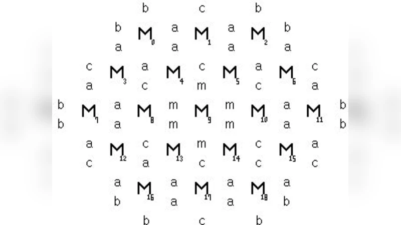
The paper applies this framework to several classic HTP configurations. The most famous example is the 30‑vertex, 3×3 diagonal layout originally studied by Choi, which has |G₁|=12, |G₂|=12, |G₃|=6 and t=12 hexagons. Substituting these numbers gives S_min = 84 and S_max = 102; the historically recorded magic constant 93 lies comfortably in the middle of this interval. The authors also analyse a 19‑vertex triangular HTP (G₁=7, G₂=8, G₃=4, t=7), a 37‑vertex star‑shaped HTP, and a larger 61‑vertex composite HTP. In each case the interval width grows with the proportion of weight‑3 vertices, confirming the intuition that more overlapping vertices increase the flexibility of S.

Beyond the theoretical bounds, the authors discuss algorithmic implications. In backtracking or constraint‑satisfaction solvers for HTP, the pre‑computed interval