Learning Deep Temporal Representations for Brain Decoding

Functional magnetic resonance imaging produces high dimensional data, with a less then ideal number of labelled samples for brain decoding tasks (predicting brain states). In this study, we propose a new deep temporal convolutional neural network architecture with spatial pooling for brain decoding which aims to reduce dimensionality of feature space along with improved classification performance. Temporal representations (filters) for each layer of the convolutional model are learned by leveraging unlabelled fMRI data in an unsupervised fashion with regularized autoencoders. Learned temporal representations in multiple levels capture the regularities in the temporal domain and are observed to be a rich bank of activation patterns which also exhibit similarities to the actual hemodynamic responses. Further, spatial pooling layers in the convolutional architecture reduce the dimensionality without losing excessive information. By employing the proposed temporal convolutional architecture with spatial pooling, raw input fMRI data is mapped to a non-linear, highly-expressive and low-dimensional feature space where the final classification is conducted. In addition, we propose a simple heuristic approach for hyper-parameter tuning when no validation data is available. Proposed method is tested on a ten class recognition memory experiment with nine subjects. The results support the efficiency and potential of the proposed model, compared to the baseline multi-voxel pattern analysis techniques.

💡 Research Summary

**
The paper tackles a fundamental challenge in functional magnetic resonance imaging (fMRI) analysis for brain decoding: the data are extremely high‑dimensional (thousands of voxels) while the number of labeled samples is very small (typically a few hundred). Traditional multi‑voxel pattern analysis (MVPA) either discards the vast majority of unlabeled time points or relies on hand‑crafted features and aggressive dimensionality reduction, which limits classification performance.

To address this, the authors propose a deep temporal convolutional neural network (CNN) that learns temporal filters in an unsupervised manner from all available fMRI time series, including the unlabeled portions, and then uses spatial pooling to dramatically reduce dimensionality before classification. The key components are:

1. Unsupervised learning of temporal filters – The full voxel‑by‑time matrix (V^T) (voxels × time) is used to sample short time windows (length (\tau_1) for the first layer, (\tau_2) for the second). Sparse autoencoders with a sparsity penalty (Kullback‑Leibler divergence) and L2 weight decay are trained to reconstruct these windows. The encoder weights become the temporal basis functions (filters). The first layer learns (k_1) filters (e.g., 8‑16) of length 6 (covering a typical hemodynamic response), while the second layer learns (k_2) filters of length 9 on the pooled outputs of the first layer.

2. Temporal convolution and spatial pooling – Each learned filter is convolved across the entire time axis of the voxel matrix, producing (k_1) response matrices of size (voxels × time). A max‑pooling operation with range (\delta_1) (e.g., 2) is applied across neighboring voxels, halving the spatial dimension and exploiting the known spatial smoothness of fMRI signals. A non‑linearity (tanh) follows. The second processing block repeats this pipeline on the pooled responses, using a second pooling range (\delta_2). After the second block, the network yields (k_1 \times k_2) pooled response matrices, each of size (\frac{m}{\delta_1 \delta_2} \times n) (where (m) is the original voxel count and (n) the number of time points). All matrices are concatenated along the feature axis, resulting in a compact representation of size (\frac{m \cdot k_2}{\delta_1 \delta_2} \times n).

3. Heuristic hyper‑parameter selection – Because a validation set is often unavailable in fMRI studies, the authors propose a rule‑of‑thumb: set the temporal window to roughly the length of the hemodynamic response (4–6 s) divided by the repetition time (TR = 2 s), yielding (\tau_1=6). Use a slightly larger window for the second layer ((\tau_2=9)) to capture higher‑level temporal patterns. Choose pooling ranges so that the final feature dimension is comparable to or smaller than the original voxel count, ensuring a fair comparison with MVPA.

4. Experimental protocol – Data were collected from nine participants performing a ten‑class recognition memory task. The region of interest was the anterior lateral temporal cortex (1024 voxels). Each participant contributed 2400 time points across eight runs, with 240 labeled samples during the encoding phase (training) and 240 during the retrieval phase (testing). No spatial smoothing or temporal filtering beyond basic motion correction was applied, preserving the raw temporal dynamics.

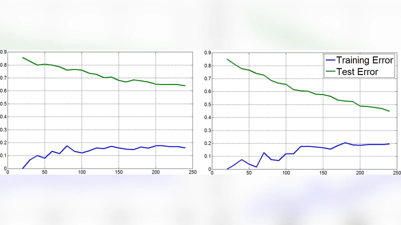
5. Results – The proposed deep temporal CNN achieved an average classification accuracy of about 62 % across subjects, outperforming standard MVPA (≈54 %) and other baselines (PCA‑SVM, ICA‑SVM) by 5–7 percentage points. The dimensionality of the learned representation was reduced to roughly 256–512 features, i.e., 2–4× smaller than the original voxel space, while still retaining discriminative information. Visual inspection of the first‑layer filters revealed shapes resembling canonical hemodynamic response functions, confirming that the unsupervised autoencoders captured physiologically meaningful temporal patterns. The second‑layer filters displayed more complex, multi‑peak structures, suggesting the network learned higher‑order temporal abstractions.

6. Discussion – The study demonstrates that (a) unlabeled fMRI time points contain valuable information that can be harvested via unsupervised learning, (b) temporal convolution combined with spatial pooling yields a compact, expressive feature space suitable for downstream linear classifiers, and (c) the learned filters are interpretable and align with known neurophysiological responses. Limitations include the reliance on 1‑D temporal convolutions (which ignore spatial correlations during convolution), potential over‑fitting of the autoencoders on limited data, and the heuristic nature of hyper‑parameter selection. The authors suggest future extensions such as 3‑D spatio‑temporal convolutions, incorporation of recurrent networks (LSTM/GRU) for longer temporal dependencies, and transfer learning across subjects to build more robust, generalizable models.

Conclusion – By integrating unsupervised temporal filter learning with a deep convolutional architecture and spatial pooling, the authors provide a novel solution to the high‑dimensional, low‑sample problem in fMRI brain decoding. The method improves classification performance over traditional MVPA while drastically reducing feature dimensionality, and it offers a physiologically plausible representation of brain activity. This work opens the door for more sophisticated deep learning pipelines in neuroimaging, especially those that can exploit the abundant unlabeled data inherent in fMRI experiments.