Robust Spectral Compressed Sensing via Structured Matrix Completion

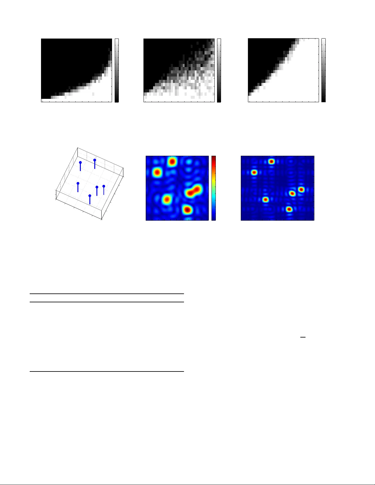
1 Rob ust Spectral Comp ressed Sensing via Structured Matrix Completion Y uxin Chen, Studen t Member , IEEE , and Y uejie Chi, Member , IEEE Abstract —The paper explores the problem of spe ctral com- pressed sensing , which aims to recov er a sp ectrally sparse signal from a small random subset of its n time domain samples. T he signal of interest is assumed to be a su perposition of r multi- dimensional complex sinusoids, while the u nderlying frequencies can assume any contin uous values in the normalized frequency domain. Conv entional compressed sensing paradigms suffer from the basis mismatch issu e when imposing a d iscrete dictionary on the Fourier representation. T o address this issue, we develop a nove l algorithm, called Enhanced Matrix Completion (E MaC) , based on stru ctured matrix completion that does not require prior kn owledge of the model order . Th e algorithm starts by arranging the data into a low-rank enhanced form exhib iting multi-fold Hankel structure, and th en attempts reco very via nuclear norm mini mization. Under mild incoherence conditions, EMaC allows perfect recov ery as soon as the number of samples exceeds th e order of r log 4 n , and is stable against bound ed noise. Ev en if a constant portion of samples are corrupted with arbitrary magnitude, EMaC still allows exact recov ery , p ro vided that the sample complexity exceeds the order of r 2 log 3 n . Along the way , our results d emonstrate the power of conv ex relaxa tion in completing a low-rank multi-fold Hankel or T oeplitz matrix fr om minimal obser ved entries. Th e p erf ormance of our algorithm and its applicabil ity to super resolution are further validated by numerical experiments. Index T erms —sp ectral compressed sensing, matrix completion, Hankel matrices, T oeplitz ma trices, basis mismatch, o ff-grid compressed sensing, incoherence, super-r esolution I . I N T RO D U C T I O N A. Motivation and Contrib utions A large class of practical applications features high- dimensiona l sign als that can be mod eled or appro ximated by a sup erposition of spikes in the spec tral (resp. time) doma in, and inv olves estimatio n of the sign al from its time (resp. frequen cy) do main sample s. Exam ples includ e acceleration of medical im aging [1] , target localiza tion in radar a nd son ar systems [2], in verse scatter ing in seismic imag ing [ 3], ﬂuo res- cence microscopy [4 ], c hannel estima tion in wire less co mmu- nications [5], analog- to-digital conversion [6], e tc. The data acquisition devices, h owe ver , are o ften limited by hardware and phy sical constrain ts, pre cluding sam pling with the desired resolution. It is thus of param ount in terest to reduce sensing complexity wh ile retaining recovery ac curacy . Y . Chen is with the Department of Electric al Engineering, Stan ford Uni- versi ty , Stanford, CA 94305, USA (email: yxchen@stanford.edu ). Y . Chi is with Department of E lectr ical and Computer E nginee ring and Departmen t of Biomedic al Informatics, The Ohio State Unive rsity , Columbus, OH 43210, USA (email: chi.97@osu.edu). Prelimina ry results of this work have been presente d at the 2013 Inter - nationa l Conferenc e on Machine L earning (ICML) and the 2013 Signal Pro- cessing with Adaptiv e Sparse Structured Representa tions W orkshop (SP ARS). Manuscript date: July 22, 2014. In this paper , we in vestigate the s pectral compr essed sensing problem , which aims to r ecover a spectrally spa rse signal f rom a small nu mber of rand omly observed time domain samples. The signal of intere st x ( t ) with ambient dimension n is assumed to be a weighted sum of m ulti-dimen sional comp lex sinusoids at r distinct f requencie s { f i ∈ [0 , 1) K : 1 ≤ i ≤ r } , where the underlying frequencies can assume any continuou s values on the unit interval. Spectral compressed sensing is closely related to the pr ob- lem o f harmon ic r etrieval , which seeks to extract the u nder- lying f requenc ies o f a signal from a co llection o f its time domain samples. Conventional me thods for harm onic re triev al include Pro ny’ s method [7], E SPRIT [ 8], the matr ix pe ncil method [9], the T ufts and Kumaresan ap proach [10], the ﬁn ite rate of innovation app roach [11], [ 12], etc. These methods routinely exploit the shift invariance of the harmon ic structure, namely , a consecutive segment of time domain samp les lies in the same subspace irr espectiv e of the startin g poin t of th e segment. Howe ver , one weakness of these techniqu es if th at they requir e prior kn owledge of th e mo del order, that is, the number o f under lying frequency spikes of the signal or at least an estimate of it. Besides, these techn iques h eavily rely on the knowledge of the no ise sp ectra, and ar e often sensitiv e against noise and outliers [13]. Another line of work is concerned with Compressed Sensing (CS) [14], [15] over a discrete domain , which suggests that it is p ossible to recover a signal even w hen the num ber of samples is far below its ambient dimension , p rovided th at the signal enjoys a sparse repr esentation in the transform d omain. In particular , tr actable alg orithms based on conve x surrog ates become po pular due to their compu tational efﬁciency and robustness against noise and outliers [16], [1 7]. Furthermor e, they do no t require prior infor mation on the mod el order . Nev ertheless, th e succ ess of CS r elies o n spa rse rep resentation or app roximation of the signal o f interest in a ﬁnite d iscrete dictionary , while the true param eters in ma ny applica tions are actually speciﬁed in a continu ous dictionary . The basis mismatch between the true frequ encies and the discretized grid [18] results in loss of spar sity due to spectral leakag e along the Dirichlet kernel, and hence d egeneration in the pe rforman ce of con ventional CS parad igms. In this paper, we develop an algorithm , ca lled En hanced Matrix Completion (EMa C) , that simultan eously explo its the shift inv ariance pr operty of harmonic structur es and the spec- tral spar sity of signals. Inspired b y the con ventiona l m atrix pencil form [19], EMaC starts by ar ranging the data samples into an enh anced ma trix exhib iting K -fold Han kel structur es, whose rank is bo unded above by the spectral sparsity r . This 2 way we con vert the spectral s parsity into the lo w-rank structure without imposing any pre-determined grid. EMaC then i nv okes a nuclear norm minimization prog ram to com plete the en- hanced matr ix from p artially ob served samp les. When a small constant propor tion of the observed samples are corrupted with arbitrary m agnitudes, EMaC solves a weigh ted nuclear norm minimization and ℓ 1 norm minimization to re cover th e signal as well as th e sparse corruption component. The perfor mance o f EMaC depen ds on an inco herence condition th at depen ds only on the frequen cy locations r e- gardless of the amplitudes of their respec ti ve c oefﬁcients. The incoheren ce m easure is character ized by th e recip rocal of the smallest singu lar value of some Gram m atrix, which is deﬁned b y sampling the Dirichlet kernel at the wrap-a round differences of all freq uency pairs. The sign al of inter est is said to o bey the incoh erence condition if the Gram matrix is well cond itioned, wh ich arises over a broad class of spectrally sparse signals inclu ding but not restricted to signals with well-separated frequenc ies. W e demon strate that, und er this incohere nce cond ition, EMaC enab les exact recovery fro m O ( r log 4 n ) ran dom samples 1 , an d is stable against b ound ed noise. Moreover , EMaC ad mits perf ect sign al recovery fro m O ( r 2 log 3 n ) rand om samples e ven when a constant propor tion of the sam ples are corr upted with arbitrar y mag nitudes. Fi- nally , n umerical experimen ts validate our th eoretical ﬁnd ings, and demon strate the applicability of EMaC in super resolution. Along the way , we p rovide theoretical guaran tees for low- rank matrix com pletion of Hankel matrices and T o eplitz matri- ces, whic h is of great importance in control, natural la nguage processing, and computer vision. T o the best of our knowledge, our results p rovide th e ﬁrst theor etical guarantees for Hankel matrix comp letion that are c lose to the infor mation theor etic limit. B. Connection and Comparison to Prior W ork The K -fo ld Hankel structure, which play s a central role in the EMaC algo rithm, r oots from the tr aditional spectral esti- mation techniqu e named Matrix Enh ancement Matrix Pen cil (MEMP) [19] for multi- dimensional harmonic retrieval. The conv ention al MEMP algo rithm assumes fully observed equi- spaced time domain samples for estimation, and require p rior knowledge o n the model o rder . Cadz ow’ s den oising method [20] also exploits the low-rank structure of the matrix pen cil form for denoising line spectrum, but the metho d is non - conv ex and lacks perfor mance guara ntees. When th e fre quencies of the signal in deed fall on a grid, CS algorithm s based on ℓ 1 minimization [14], [15] assert th at it is possible to recover the spectra lly sparse signal from O ( r log n ) random time dom ain samp les. Th ese algo rithms admit faithful recovery ev en whe n the samp les are con taminated by bound ed noise [ 16], [ 21] or arbitra ry sparse outliers [17]. Whe n the inevitable b asis misma tch issue [18 ] is presen t, se veral r eme- dies of CS algo rithms have bee n p roposed to mitigate the 1 The standard notation f ( n ) = O ( g ( n )) means that there exists a constant c > 0 such that f ( n ) ≤ c g ( n ) ; f ( n ) = Θ ( g ( n )) indic ates that there ar e numerica l constants c 1 , c 2 > 0 such that c 1 g ( n ) ≤ f ( n ) ≤ c 2 g ( n ) . effect [22], [23] under random li near pr ojection measurements, although theoretical guarantees are in ge neral lac king. More recently , Candï¿œs and Fernandez- Granda [24] pro- posed a total-v ariation norm minimizatio n algor ithm to super- resolve a spar se sign al from frequ ency samples at th e low end of the spectrum. This algorithm allows accurate super- resolution wh en the point sources ar e sufﬁciently separated , and is stable against noise [2 5]. Inspired b y this approac h, T ang et. al. [ 26] th en developed an atomic norm min imization algorithm f or line sp ectral estimation from O ( r log r lo g n ) random time domain samples, which enab les exact recovery when the freq uencies are separated by at least 4 /n with random a mplitude phases. Similar pe rforman ce guaran tees are later estab lished in [2 7] for multi-d imensional freq uencies. Howe ver , the se results are established u nder a rando m signal model, i. e. the co mplex signs o f the f requency spikes are assumed to be i.i.d. drawn from a unifo rm distribution. The robustness of the method ag ainst n oise and outliers is not established either . In con trast, our app roach yields deter min- istic cond itions for multi-dim ensional fr equency mod els that guaran tee perfect recovery with noiseless samples an d are provably robust again st n oise an d sparse corruptions. W e will provide d etailed comp arison with the appro ach of T an g et. al. after we forma lly pr esent our resu lts. Numer ical compa rison will also be p rovided in Section V - C for the line sp ectrum model. Our algorithm is inspire d by recent advances of M atrix Completion (MC) [28], [29], which aims at recovering a lo w- rank matrix from partial entries. It has been shown [3 0]–[32] that exact recovery is po ssible via nuclear no rm m inimization, as soon as the num ber of observed en tries exceeds the order of the inform ation theo retic limit. Th is line of algorithms is also robust aga inst noise and outliers [3 3], [34], and allows exact recovery even in th e presence of a co nstant por tion of adversarially cor rupted entrie s [3 5]–[37], wh ich have fou nd numero us applications in collabo rative ﬁltering [38], medical imaging [39], [40], etc. Nevertheless, the theo retical g uaran- tees of these algorithms do not apply to the mo re stru ctured observation models associated with the prop osed multi-fold Hankel structure. Consequen tly , direct app lication of existing MC results d eliv ers p essimistic sample complexity , which far exceeds the d egrees of freedo m un derlying the sign al. Preliminary results of this work have been presente d in [41], wher e an a dditional stro ng inco herence cond ition was introdu ced that bo re a similar role as the tradition al strong incohere nce parameter in MC [30] but lacked phy sical in- terpretation s. Th is paper r emoves this con dition and f urther improves the sample complexity . C. Organization The rest of th e pap er is organized as follows. The signal an d sampling mod els are d escribed in Sec tion II. By restricting our attention to two-dimensional (2-D) frequen cy models, we present the enhan ced matrix fo rm and the associated struc- tured matrix completio n algor ithms. Th e extension to mu lti- dimensiona l frequen cy mo dels is discussed in Section III -C. The main theor etical guaran tees are su mmarized in Section 3 III, based on the in coherence condition introduced in Section III-A. W e then d iscuss the extension to low-rank Hankel an d T oeplitz matrix c ompletion in Section IV. Section V p resents the nu merical validation of o ur algorith ms. Th e proo fs of Theorem s 1 and 3 are based on duality an alysis followed by a golﬁng scheme, wh ich a re sup plied in Section VI a nd Section VII, respectiv ely . Section VIII concludes the paper wit h a short summary of o ur ﬁndings as well as a discussion of potential extensions an d improvements. Fina lly , the proofs o f auxiliary lemmas supp orting our results are defer red to th e app endices. I I . M O D E L A N D A L G O R I T H M Assume that the signal of interest x ( t ) can be modeled as a weigh ted sum of K -dimensional complex sinusoids at r distinct frequen cies f i ∈ [0 , 1) K , 1 ≤ i ≤ r , i. e. x ( t ) = r X i =1 d i e j 2 π h t , f i i , t ∈ Z K . (1) It is assum ed th rougho ut that the freq uencies f i ’ s are nor- malized with respect to the Nyq uist fre quency of x ( t ) an d the time domain m easurements ar e sample d at in teger values. W e deno te b y d i ’ s the co mplex amplitu des o f the associated coefﬁcients, and h· , ·i r epresents the inn er p roduct. For con- creteness, o ur discussion is ma inly devoted to a 2-D fr equency model wh en K = 2 . This sub sumes line spectral estima- tion a s a specia l ca se, a nd indica tes h ow to add ress multi- dimensiona l mo dels. The algor ithms for higher dime nsional scenarios clo sely parallel the 2-D case, which will b e brieﬂy discussed in Section III-C. A. 2-D F requency Model Consider a data matrix X = [ X k,l ] 0 ≤ k min ( n 1 , n 2 ) . This motivates us to seek o ther forms that better capture the har monic structure. In this paper, we ad opt one effecti ve enh anced form of X based on the fo llowing two-fold Hankel structure. T he enhanced ma trix X e with resp ect to X is deﬁned as a k 1 × ( n 1 − k 1 + 1) block Hankel m atrix X e :=      X 0 X 1 · · · X n 1 − k 1 X 1 X 2 · · · X n 1 − k 1 +1 . . . . . . . . . . . . X k 1 − 1 X k 1 · · · X n 1 − 1      , (8) where k 1 (1 ≤ k 1 ≤ n 1 ) is called a pen cil par ameter . E ach block is a k 2 × ( n 2 − k 2 + 1) Hankel matrix deﬁned such th at for e very ℓ ( 0 ≤ ℓ < n 1 ): X ℓ :=      X ℓ, 0 X ℓ, 1 · · · X ℓ,n 2 − k 2 X ℓ, 1 X ℓ, 2 · · · X ℓ,n 2 − k 2 +1 . . . . . . . . . . . . X ℓ,k 2 − 1 X ℓ,k 2 · · · X ℓ,n 2 − 1      , (9) where 1 ≤ k 2 ≤ n 2 is another pencil parameter . This enhanced form allo ws us to e xpr ess ea ch block as 2 X ℓ = Z L Y ℓ d D Z R , (10) 2 Note that the l th ( 0 ≤ l < n 1 ) row X l ∗ of X can be expressed as X l ∗ = h y l 1 , · · · , y l r i D Z ⊤ = h y l 1 d 1 , · · · , y l r d r i Z ⊤ , and hence we only need to ﬁnd the V andemonde decomposition for X 0 and then replace d i by y l i d i . 4 where Z L , Z R and Y d are deﬁned respectiv ely as Z L :=      1 1 · · · 1 z 1 z 2 · · · z r . . . . . . . . . . . . z k 2 − 1 1 z k 2 − 1 2 · · · z k 2 − 1 r      , Z R :=      1 z 1 · · · z n 2 − k 2 1 1 z 2 · · · z n 2 − k 2 2 . . . . . . . . . . . . 1 z r · · · z n 2 − k 2 r      , and Y d := diag [ y 1 , y 2 , · · · , y r ] . Substituting (10) into (8) yields the fo llowing: X e =      Z L Z L Y d . . . Z L Y k 1 − 1 d      | {z } √ k 1 k 2 E L D  Z R , Y d Z R , · · · , Y n 1 − k 1 d Z R  | {z } √ ( n 1 − k 1 +1)( n 2 − k 2 +1) E R , (11) where E L and E R span the column and r ow space of X e , respectively . This immediately implies that X e is low-rank , i.e. rank ( X e ) ≤ r. (12) This f orm is in spired by th e trad itional matrix p encil ap proach propo sed in [9], [19] to estimate har monic f requenc ies if all entries of X ar e av ailable. Thus, one can extract all underlying frequen cies of X using methods p roposed in [19], as long as X can be faithfully recovered. C. The EMaC Algorithm in the Ab sence of Noise W e th en attempt recovery through th e following Enhan ce- ment Matrix Completion (EMaC) a lgorithm: (EMaC) minimize M ∈ C n 1 × n 2 k M e k ∗ (13) subject to P Ω ( M ) = P Ω ( X ) , where M e denotes the enh anced form o f M . I n other words, EMaC minimize s the nuclear norm o f th e enhan ced f orm over all matrices compatible with t he samples. This con vex pr ogram can be rewritten into a semideﬁnite program (SDP) [4 2] minimize M ∈ C n 1 × n 2 1 2 T r ( Q 1 ) + 1 2 T r ( Q 2 ) subject to P Ω ( M ) = P Ω ( X ) ,  Q 1 M ∗ e M e Q 2   0 , which can be solved using off-the-shelf solvers in a tractable manner (see, e. g., [ 42]). I t is worth m entioning th at EMaC has a similar com putational complexity as th e ato mic norm m in- imization method [26] wh en re stricted to the 1-D freq uency model. Careful readers will remark tha t th e per forman ce o f EMaC must d epend on the choices of the p encil par ameters k 1 and k 2 . In fact, if we deﬁne a quantity c s := max  n 1 n 2 k 1 k 2 , n 1 n 2 ( n 1 − k 1 + 1) ( n 2 − k 2 + 1)  (14) that m easures h ow close X e is to a squ are matrix , then it will be shown later tha t the requ ired samp le comp lexity for faithful recovery is an increasing func tion o f c s . In fact, both our theor y and em pirical experiments are in fav or of a small c s , correspon ding to the choices k 1 = Θ ( n 1 ) , n 1 − k 1 + 1 = Θ ( n 1 ) , k 2 = Θ ( n 2 ) , and n 2 − k 2 + 1 = Θ ( n 2 ) . D. Th e Noisy-EMaC Algorithm wit h Bou nded Noise In practice, me asurements are ofte n con taminated by a certain a mount of no ise. T o make o ur mo del and algor ithm more practically applicable, we r eplace our measurements by X o = [ X o k,l ] 0 ≤ k 0 is a regularization parameter that will be s peciﬁed later . As will be shown later, λ can be selected in a p arameter- free fashion. W e denote by M e and ˆ S e the en hanced form of M and ˆ S , respecti vely . Here, k ˆ S e k 1 := k vec ( ˆ S e ) k 1 represents the elemen twise ℓ 1 -norm of ˆ S e . Robust-EMaC pr omotes the low-rank structure of th e enhanced data matrix as well as th e sparsity of the outliers via conve x r elaxation with respective structures. F . Notation s Before con tinuing, we introdu ce a few notation s that will b e used thro ughou t. Le t the singular v alue decom position (SVD) of X e be X e = U Λ V ∗ . Denote by T : = n U M ∗ + ˜ M V ∗ : M ∈ C ( n 1 − k 1 +1)( n 2 − k 1 +1) × r , ˜ M ∈ C k 1 k 2 × r o (19) the tangent space with respect to X e , and T ⊥ the o rthogo nal compleme nt of T . Denote by P U (resp. P V , P T ) the orthog- onal projection onto the colu mn ( resp. row , tan gent) space of X e , i.e. for any M , P U ( M ) = U U ∗ M , P V ( M ) = M V V ∗ , and P T = P U + P V − P U P V . W e let P T ⊥ = I − P T be th e orthogonal complem ent o f P T , where I denote s the identity opera tor . Denote by k M k , k M k F and k M k ∗ the spectral norm (operato r no rm), Froben ius nor m, and nucle ar n orm of M , respectively . Also, k M k 1 and k M k ∞ are d eﬁned to be the elementwise ℓ 1 and ℓ ∞ norm of M . Den ote by e i the i th standard basis vector . Additionally , we use sgn ( M ) to den ote the elementwise complex sign of M . On the other hand, we denote by Ω e ( k , l ) the set of locations of the enha nced m atrix X e containing copies of X k,l . Due to the Hankel or mu lti-fold Hankel structures, one can easily verify t he following: each location set Ω e ( k , l ) co ntains at most one index in any given row o f the enh anced fo rm, and at mo st one index in any given column . For each ( k , l ) ∈ [ n 1 ] × [ n 2 ] , we use A ( k,l ) to denote a basis ma trix that extracts the av erage of all entries in Ω e ( k , l ) . Spe ciﬁcally ,  A ( k,l )  α,β := ( 1 √ | Ω e ( k,l ) | , if ( α, β ) ∈ Ω e ( k , l ) , 0 , else . (20) W e will use ω k,l := | Ω e ( k , l ) | (21) throug hout as a short-h and no tation. I I I . M A I N R E S U LT S This section d eli vers the fo llowing encouraging news : un der mild in coheren ce co nditions, E MaC e nables faithfu l signal recovery from a minimal num ber of time-do main samp les, ev en when the samples ar e co ntaminated b y bou nded no ise or a constant portion of ar bitrary outliers. A. Incoherence Mea sur e In gen eral, matrix co mpletion fro m a f e w en tries is ho peless unless the underlyin g structure is s ufﬁciently uncorrelated with the observation basis. This inspires us to intro duce certain incohere nce measures. T o this end, we deﬁn e the 2-D Dirichlet kernel as D ( k 1 , k 2 , f ) := 1 k 1 k 2  1 − e − j 2 π k 1 f 1 1 − e − j 2 π f 1   1 − e − j 2 π k 2 f 2 1 − e − j 2 π f 2  , (22) where f = ( f 1 , f 2 ) ∈ [0 , 1) 2 . Fig. 1 (a) illustrates the amplitude o f D ( k 1 , k 2 , f ) when k 1 = k 2 = 6 . The value of |D ( k 1 , k 2 , f ) | de cays inverse pr oportio nally with respect to the frequ ency f . Set G L and G R to be two r × r Gr am matrices such that their en tries are speciﬁed r espectiv ely by ( G L ) i,l = D ( k 1 , k 2 , f i − f l ) , ( G R ) i,l = D ( n 1 − k 1 + 1 , n 2 − k 2 + 1 , f i − f l ) , where th e d ifference f i − f l is under stood as the wrap-ar ound distance in the inter val [ − 1 / 2 , 1 / 2 ) 2 . Simple manipu lation reveals that G L = E ∗ L E L , G R = ( E R E ∗ R ) ⊤ , where E L and E R are deﬁned in ( 11). Our incoheren ce measure is then deﬁned as follo ws. Deﬁnition 1 ( Incoherence ) . A ma trix X is said to obey the incoherence p r operty with parameter µ 1 if σ min ( G L ) ≥ 1 µ 1 and σ min ( G R ) ≥ 1 µ 1 . (23) wher e σ min ( G L ) and σ min ( G R ) r epr esent the least singular values of G L and G R , r espectively . The incoher ence measur e µ 1 only depen ds o n th e locations of the frequen cy spikes, irrespective of the amplitudes of their r espectiv e coefﬁcients. The signal is said to satisfy the incoher ence condition if µ 1 scales as a small constant, which occurs when G L and G R are b oth well-condition ed. Our incoherence condition naturally requires certain separation among all fre quency pair s, as when two freq uency spikes are closely located, µ 1 gets undesirably large. As shown in [43, T heorem 2 ], a separation of a bout 2 / n fo r line spectrum is sufﬁcient to guaran tee the incohere nce conditio n to hold . Howe ver , it is worth em phasizing that su ch strict separation is not necessary as requir ed in [26], and th ereby o ur incoher ence condition is applicable to a broade r class of spe ctrally sparse signals. T o give the reader a ﬂavor o f the in coheren ce condition , we list two examp les b elow . For ease of presentation, we assume below 2-D freque ncy mo dels with n 1 = n 2 . Note, howe ver , 6 2 4 6 8 10 12 14 16 18 0 0.1 0.2 0.3 0.4 0.5 0.6 0.7 0.8 0.9 1 sparsity level minimum eigenvalue of G L k = 6 k = 36 k = 72 (a) (b) Fig. 1. (a) T he 2-D Dirichlet kernel when k = k 1 = k 2 = 6 ; (b) The empirical distributi on of the minimum eigen value σ min ( G L ) for vari ous choice s of k with respect to the sparsity lev el. that the asy mmetric cases an d general K -dim ensional fre- quency models can be analyze d in the same manne r . • Ran dom fr equ ency locatio ns : supp ose that the r fre- quencies are g enerated unifo rmly at rand om, the n the minimum pairwise separation can be crudely bou nded b y Θ  1 r 2 log n 1  . If n 1 ≫ r 2 . 5 log n 1 , then a crud e bou nd reveals that ∀ i 1 6 = i 2 , max ( 1 k 1 1 −  y ∗ i 1 y i 2  k 1 1 − y ∗ i 1 y i 2 , 1 k 2 1 −  z ∗ i 1 z i 2  k 2 1 − z ∗ i 1 z i 2 ) ≪ 1 √ r holds with high p robability , indicating that the off- diagona l e ntries of G L and G R are much smaller than 1 /r in magnitu de. Simple manipulatio n th en allows u s to conclud e that σ min ( G L ) and σ min ( G R ) are bound ed b e- low by positive co nstants. Fig. 1 (b ) shows the minimu m eigenv alue of G L for d ifferent k = k 1 = k 2 = 6 , 36 , 72 when the spikes are randomly genera ted an d th e nu mber of spikes is given as the sparsity level. The m inimum eigenv alue o f G L gets clo ser to one as k grows, con ﬁrm- ing our argument. • Sma ll perturba tion off the grid : supp ose that all f requen- cies are within a d istance at most 1 n 1 r 1 / 4 from some grid points  l 1 k 1 , l 2 k 2  (0 ≤ l 1 < k 1 , 0 ≤ l 2 < k 2 ) . One can verify that ∀ i 1 6 = i 2 , max ( 1 k 1 1 −  y ∗ i 1 y i 2  k 1 1 − y ∗ i 1 y i 2 , 1 k 2 1 −  z ∗ i 1 z i 2  k 2 1 − z ∗ i 1 z i 2 ) < 1 2 √ r , and hence th e magnitu de of all off-diago nal entries of G L and G R are no larger tha n 1 / (4 r ) . This immediately sug- gests that σ min ( G L ) and σ min ( G R ) are lower bo unded by 3 / 4 . Note, howev er, that the class of incoh erent sign als are far beyond th e ones discussed a bove. B. Theor etical Guarantees W ith the above incohere nce measur e, the ma in theo retical guaran tees are provid ed in the following thre e theorems each accountin g for a distinct da ta mod el: 1) noiseless measu re- ments, 2) measurem ents contaminated by b ounded no ise, and 3) m easurements corrup ted by a constant prop ortion of arbitrary outliers. 1) Exa ct Recovery fr o m Noiseless Measurements: E xact recovery is possible fr om a minimal nu mber of noise-free samples, as asserted in the fo llowing theore m. Theorem 1 . Let X be a data matrix of form ( 3), and Ω the random location set of size m . Supp ose that the incoherence pr operty (23) hold s and th at all measurements ar e no iseless. Then th er e exists a u niversal con stant c 1 > 0 such that X is the un ique solution to E MaC with pr obab ility e xceedin g 1 − ( n 1 n 2 ) − 2 , pr ovided that m > c 1 µ 1 c s r log 4 ( n 1 n 2 ) . (24) Theorem 1 asserts that un der som e mild d eterministic incohere nce condition suc h th at µ 1 scales as a small constant, EMaC ad mits prefe ct recovery as soon as the numb er of measuremen ts exceeds O ( r log 4 ( n 1 n 2 )) . Since th ere are Θ ( r ) degrees of f reedom in tota l, the lower bound shou ld be no smaller th an Θ ( r ) . This d emonstrates the order wise optim ality of EMaC except f or a logar ithmic gap . W e note, howev er, th at the p olylog factor might be furth er reﬁned via ﬁner tuning of concentr ation of measure inequalities. It is w orth emphasizing that while we assum e random o bser- vation m odels, the data model is assumed deterministic. This differs sign iﬁcantly fro m [26], wh ich r elies on r andomn ess in both the o bservation model and the d ata model. In particular, our theoretical perfor mance guaran tees rely solely on the frequen cy location s ir respective of th e associated amplitu des. In co ntrast, the results in [2 6] r equire the phases of all frequen cy sp ikes to be i.i.d. drawn in a unif orm m anner in addition to a separation condition. Remark 1 . Theorem 1 signiﬁcantly stren gthens our prior results rep orted in [41] by improving the requ ired sample comp lexity from O  µ 2 1 c 2 s r 2 poly lo g( n 1 n 2 )  to O ( µ 1 c s r po ly log( n 1 n 2 )) . 2) Sta ble Recovery in th e Pr esence o f Bound ed Noise: Our method enable s stable recovery even wh en the time domain samples are noisy co pies o f the true data. He re, we say the recovery is stable if the solution o f Noisy -EMaC is clo se to the ground truth in pro portion to the noise le vel. T o th is end, we p rovide the following theor em, which is a cou nterpart of Theorem 1 in the no isy setting, whose pro of is inspired by [44]. Theorem 2. Sup pose X o is a noisy copy of X tha t satisﬁes kP Ω ( X − X o ) k F ≤ δ . Un der the con ditions of Theo r em 1, the solution to Noisy-EMaC in (1 6) satisﬁes k ˆ X e − X e k F ≤ 5 n 3 1 n 3 2 δ (25) with pr obability exceeding 1 − ( n 1 n 2 ) − 2 . Theorem 2 reveals tha t the recovered e nhanced matrix (which contain s Θ( n 2 1 n 2 2 ) entries) is close to the true en hanced matrix at h igh SNR. In pa rticular, the average entry inaccu racy of the enhanced matrix is bound ed above by O ( n 3 1 n 3 2 δ ) , ampli- ﬁed by the sub sampling factor . I n practice, one is in terested in an estimate o f X , which ca n b e o btained n aiv ely b y rando mly selecting an entry in Ω e ( k , l ) as ˆ X k,l , then we ha ve k ˆ X − X k F ≤ k ˆ X e − X e k F . 7 This y ields that the per-entry no ise o f ˆ X is abo ut O ( n 2 . 5 1 n 2 . 5 2 δ ) , which is f urther am pliﬁed d ue to enha ncement by a factor of n 1 n 2 . Howe ver , this factor arises fro m an anal- ysis artifact due to our simp le strategy to ded uce ˆ X f rom ˆ X e , and may be ele vated. W e note that in n umerical experiments, Noisy-EMaC u sually g enerates mu ch better estimates, usually by a poly nomial factor . T he practical applicab ility will be illustrated in Section V. It is worth mentionin g that to the b est o f our knowledge, our result is the ﬁrst stability result with partially observed data f or spectra l comp ressed sensing off the grid. While the atomic norm approach is n ear-minimax with full data [45], it is not clear ho w it performs with partially ob served data . 3) Robust Recovery in th e P r esence of Spa rse Outliers: Interestingly , Robust-EMaC can provably tolera te a constant portion of ar bitrary o utliers. T he th eoretical perf ormance is formally summarized in th e following theo rem. Theorem 3. Let X be a da ta matrix with matrix form (3), a nd Ω a random loc ation set o f size m . Set λ = 1 √ m log( n 1 n 2 ) , and assume τ ≤ 0 . 1 is some sma ll positive constan t. Then ther e exis t a numerical constant c 1 > 0 depen ding only on τ such that if (23) holds and m > c 1 µ 2 1 c 2 s r 2 log 3 ( n 1 n 2 ) , (26) then Robust-EMaC is exact, i.e. the minimizer ( ˆ M , ˆ S ) satisﬁes ˆ M = X , with pr o bability e xceeding 1 − ( n 1 n 2 ) − 2 . Remark 2 . Note that τ ≤ 0 . 1 is not a critical threshold. I n fact, one can prove the same theor em f or a larger τ (e.g . τ ≤ 0 . 25 ) with a larger absolute constant c 1 . Howe ver , to allow even larger τ (e.g. in the regime wh ere τ ≥ 50% ), we need the sparse compo nents exhibit random sign patter ns. Theorem 3 speciﬁes a can didate cho ice of the regularization parameter λ th at allows recovery fro m a few samples, which only depend s on the size of Ω but is otherw ise parameter- free. In practice, howe ver , λ ma y better b e selected via cross validation. Fur thermore, T heorem 3 demo nstrates th e possibility of ro bust recovery un der a co nstant propo rtion of sparse co rruption s. Un der the same m ild inco herence con - dition as for Th eorem 1, ro bust recovery is p ossible from O  r 2 log 3 ( n 1 n 2 )  samples, even when a con stant prop ortion of the sam ples are arbitrar ily co rrupted. As far as w e kno w , th is provides the ﬁrst theoretical gu arantees fo r sepa rating sparse measuremen t corru ptions in the off-grid compr essed sensing setting. C. Extension to Hig her-Dimensional and Damping F requency Models By letting n 2 = 1 the ab ove 2-D freq uency model r ev erts to the line spectru m mod el. T he EMaC algorithm and the main results immed iately extend to h igher dim ensional fre- quency mod els withou t difﬁculty . In fact, f or K -dimen sional frequen cy mod els, on e can a rrange the original data into a K - fold Han kel matrix of rank at mo st r . For instance, co nsider a 3-D model such that X l 1 ,l 2 ,l 3 = r X i =1 d i y l 1 i z l 2 i w l 3 i , ∀ ( l 1 , l 2 , l 3 ) ∈ [ n 1 ] × [ n 2 ] × [ n 3 ] . An enhanced for m can be d eﬁned as a 3- fold Hankel matr ix such that X e :=      X 0 , e X 1 , e · · · X n 3 − k 3 , e X 1 , e X 2 , e · · · X n 3 − k 3 +1 , e . . . . . . . . . . . . X k 3 − 1 , e X k 1 , e · · · X n 3 − 1 , e      , where X i, e denotes the 2-D enha nced f orm of the m atrix consisting of all entries X l 1 ,l 2 ,l 3 obeying l 3 = i . One can verify that X e is of rank at most r , and can the reby app ly EMaC on the 3- D enhanced form. T o summ arize, for K - dimensiona l freq uency m odels, EMaC (re sp. Noisy-EMaC, Robust-EMaC) searches over all K -f old Han kel matrices that are c onsistent with th e measurements. T he theoretical perfor mance gu arantees can be similarly extended by deﬁning the re spectiv e Dirichlet kern el in 3- D and the coh erence measure. In fact, a ll our analyses can be extended to handle damping modes, when the frequen cies are not of time-in variant amplitudes. W e omit the details for conciseness. I V . S T RU C T U R E D M AT R I X C O M P L E T I O N One prob lem clo sely related to ou r method is com pletion of mu lti-fold Han kel matrices fr om a small numbe r o f entries. While each spectrally spa rse signal can be map ped to a low- rank multi- fold Hankel matrix, it is not clear wheth er all multi-fold Hankel matrices of ran k r can b e written as the enhanced form o f a signal with spe ctral sparsity r . Therefore, one can think of recovery o f multi-fold Hankel matrices as a more general problem than th e sp ectral compressed sensing problem . In deed, Hankel ma trix comp letion has found n umer- ous applications in system identiﬁcation [46], [47], natural languag e processing [48], computer vision [4 9], m agnetic resonance imaging [50], etc. There h as been se veral work co ncerning algorith ms an d numerical experiments for Ha nkel m atrix completions [46], [47], [51]. Howev er, to the b est of ou r k nowledge, there has be en little the oretical gua rantee that ad dresses directly Hankel matrix com pletion. Our analysis framework can be straightfor wardly ad apted to th e gen eral K -f old Hankel matrix completion s. Below we present the perform ance guaran tee for th e two-fold Han kel matrix comp letion without loss o f generality . Notice that we need to modif y the de ﬁnition of µ 1 as stated in th e following theor em. Theorem 4. Con sider a two-fold Hankel matrix X e of rank r . The bo unds in Theor ems 1, 2 and 3 co ntinue to hold, if the incoherence µ 1 is deﬁned as the smallest n umber tha t satisﬁes max ( k,l ) ∈ [ n 1 ] × [ n 2 ]  k U ∗ A ( k,l ) k 2 F , k A ( k,l ) V k 2 F  ≤ µ 1 c s r n 1 n 2 . (27) Condition (27) r equires that the left and righ t singular vectors are suf ﬁciently uncorrelated with the observation basis. In fact, con dition (27) is a weaker assumption than (23). It is worth men tioning that a low-rank Hankel matrix can often be converted to its low-rank T oeplitz counterp art, by reversely ord ering all rows o f th e Han kel matrix . Both Hankel and T o eplitz matrices ar e effecti ve form s th at capture the under lying harmo nic structur es. Our results and ana lysis 8 framework extend to low-rank T oe plitz matrix co mpletion problem without difﬁculty . V . N U M E R I C A L E X P E R I M E N T S In this section, we presen t numerical examples to ev aluate the perfor mance o f EMaC and its variants u nder d ifferent scenarios. W e furth er examine the ap plication of EMaC in image super r esolution. Finally , we prop ose an extension of singular value thr esholding (SVT) de veloped by Cai et. al. [52] that exploits the mu lti-fold Hankel structure to h andle larger scale data sets. A. Phase T ransition in the Noiseless Setting T o ev aluate the p ractical ability of the EMaC algor ithm, we con ducted a serie s of num erical experimen ts to examine the phase tran sition f or exact r ecovery . Let n 1 = n 2 , an d we take k 1 = k 2 = ⌈ ( n 1 + 1) / 2 ⌉ which co rrespond s to the smallest c s . For ea ch ( r, m ) pair, 100 Mon te Carlo trials were cond ucted. W e gen erated a spectrally sparse data matrix X by rando mly gen erating r f requency spikes in [0 , 1) × [0 , 1) , and sampled a sub set Ω of size m en tries unifor mly at rand om. The EMaC a lgorithm was c onducted using the con vex p rogramm ing modeling software CVX with the in terior-point solver SDPT3 [ 53]. Each trial is decla red successful if the nor malized mean squared err or (NMSE) satisﬁes k ˆ X − X k F / k X k F ≤ 10 − 3 , whe re ˆ X den otes the estimate retu rned by E MaC. The empir ical success rate is calculated by a veraging ov er 100 Monte Carlo trials. Fig. 2 illustrates the results o f these Monte Carlo experi- ments when the dimen sions 3 of X are 11 × 11 and 15 × 15 . The horizontal axis correspond s to the number m of samples revealed to the algorithm , while the vertical axis corr esponds to the spectral sparsity level r . The emp irical success rate is reﬂected b y th e co lor o f each cell. It can b e seen f rom th e p lot that th e nu mber of samples m grows app roximately lin early with r espect to the spectral sparsity r , an d that the slopes of the phase transition lines for two cases are approx imately the same. These observations are in lin e with ou r th eoretical guaran tee in Theorem 1. Th is phase tran sition diagr ams justify the pra ctical applicability of our alg orithm in the no iseless setting. B. Stable Recovery fr om Noisy Data Fig. 3 further examin es th e stability o f the pro posed al- gorithm by p erformin g N oisy-EMaC with respect to dif ferent parameter δ on a noise-free dataset of r = 4 complex s inusoid s with n 1 = n 2 = 11 . The numbe r of random samp les is m = 5 0 . The reconstruc ted NMSE grows ap proxim ately line ar with respect to δ , validating the stability of the propo sed algorithm . 3 W e choose the dimension of X to be odd simply to yield a squared matrix X e . In fact, our results do not rely on n 1 or n 2 being either odd or prime. W e note that when n 1 and n 2 are kno wn to be prime numbers, there m ight exi st computat ionally cheaper m ethods to enable perfect recov ery (e.g. [54]) m: number of samples r: sparsity level 20 40 60 80 100 120 2 4 6 8 10 12 14 16 0 0.1 0.2 0.3 0.4 0.5 0.6 0.7 0.8 0.9 1 m: number of samples r: sparsity level 20 40 60 80 100 120 140 160 180 200 2 4 6 8 10 12 14 16 18 20 22 0 0.1 0.2 0.3 0.4 0.5 0.6 0.7 0.8 0.9 1 (a) (b) Fig. 2. Phase transition plots where frequency locati ons are randomly generat ed. T he plo t (a) conc erns the case where n 1 = n 2 = 11 , where as the plot (b) corresponds to the situation where n 1 = n 2 = 15 . The empirical success rate is calculate d by averag ing ove r 100 Monte Carlo trials. 10 −3 10 −2 10 −1 10 0 10 1 10 −5 10 −4 10 −3 10 −2 10 −1 10 0 δ NMSE Fig. 3. The reconstructi on NMSE with respect to δ for a dataset with n 1 = n 2 = 11 , r = 4 and m = 50 . C. Comp arison with Existing A ppr oaches for Line Sp ectrum Estimation Suppose that we rando mly observe 64 entries of an n - dimensiona l vector ( n = 127 ) composed of r = 4 m odes. For such 1-D signals, we comp are EMaC with the ato mic norm approa ch [2 6] as well as basis pursuit [ 55] assum ing a g rid of size 2 12 . For the atomic no rm and th e EMaC algorithm , the modes are recovered v ia linear p rediction using the re covered data [56]. Fig. 4 demonstrates th e recovery of mode lo cations for three cases, n amely when (a) all the mode s are on the DFT grid alo ng th e unit circle; (b) all the m odes are on the unit circle excep t two c losely located mo des th at are off the presum ed grid; (c) all the modes are on the u nit cir cle except tha t one o f the two closely located m odes is a damp ing mode with amplitu de 0 . 99 . In all cases, th e EMaC algorithm successfully recovers the underlying m odes, wh ile the atomic norm app roach fails to recover damp ing modes, an d basis pursuit fails with bo th off-the-grid modes and da mping modes. W e f urther com pare the ph ase tran sition of the EMaC algo- rithm an d th e atom ic n orm ap proach in [26] for line spectru m estimation. W e assume a 1-D signal of length n = n 1 = 127 and the pen cil p arameter k 1 of EMaC is ch osen to be 64 . Th e phase transition exp eriments are condu cted in the same man ner as Fig. 2. In the ﬁrst ca se, the spikes are ge nerated r andomly as Fig. 2 on a un it circle; in the second ca se, the spikes are gene rated u ntil a separation co ndition is satisﬁed ∆ := min i 1 6 = i 2 | f i 1 − f i 2 | ≥ 1 . 5 /n . Fig. 5 (a) and (b ) illustrate the phase tran sition of EMaC a nd the ato mic norm ap proach when the frequencies ar e randomly generated witho ut imposing the separation condition . The perf ormance o f the atomic no rm 9 −1 −0.5 0 0.5 1 −1 −0.5 0 0.5 1 0 0.2 0.4 0.6 0.8 1 1.2 actual −1 −0.5 0 0.5 1 −1 −0.5 0 0.5 1 0 0.2 0.4 0.6 0.8 1 1.2 hankel −1 −0.5 0 0.5 1 −1 −0.5 0 0.5 1 0 0.2 0.4 0.6 0.8 1 1.2 atomic −1 −0.5 0 0.5 1 −1 −0.5 0 0.5 1 0 0.2 0.4 0.6 0.8 1 1.2 BP −1 −0.5 0 0.5 1 −1 −0.5 0 0.5 1 0 0.2 0.4 0.6 0.8 1 1.2 actual −1 −0.5 0 0.5 1 −1 −0.5 0 0.5 1 0 0.2 0.4 0.6 0.8 1 1.2 hankel −1 −0.5 0 0.5 1 −1 −0.5 0 0.5 1 0 0.2 0.4 0.6 0.8 1 1.2 atomic −1 −0.5 0 0.5 1 −1 −0.5 0 0.5 1 0 0.2 0.4 0.6 0.8 1 1.2 BP −1 −0.5 0 0.5 1 −1 −0.5 0 0.5 1 0 0.5 1 1.5 actual −1 −0.5 0 0.5 1 −1 −0.5 0 0.5 1 0 0.5 1 1.5 hankel −1 −0.5 0 0.5 1 −1 −0.5 0 0.5 1 0 0.5 1 1.5 atomic −1 −0.5 0 0.5 1 −1 −0.5 0 0.5 1 0 0.5 1 1.5 BP (a) On-the-grid (b) Frequency misma tch (c) Frequency and Dampin g m ismatch Fig. 4. Recov ery of mode locati ons when (a) all the modes are on the DFT grid along the unit circle; (b) all the modes are on the unit circle except two closely locate d modes that are off the DFT grid; (c) all the m odes are on the unit circle excep t that one of the two closely locate d modes is a damping mode. The panels from the upper left, clockwise, are the ground truth, the E MaC algorithm, the atomic norm approach [26], and basis pursuit [55 ] assuming a grid of size 2 12 . approa ch degenerates se verely wh en the separatio n condition is n ot me t; o n th e other ha nd, the E MaC g iv es a sharp phase transition similar to the 2D case. When the sep aration condition is imposed, the p hase tran sition of th e atom ic norm approa ch greatly improves as shown in Fig. 5 (c), while the phase tran sition o f EMaC still gives similar perfo rmance as in Fig. 5 (a) (W e o mit the actual phase tran sition in this case.) Howe ver , it is worth men tioning that wh en the sparsity level is relativ ely high , the req uired separation con dition is in general difﬁcult to be satisﬁed in p ractice. In co mparison, EMaC is less sensiti ve to the sep aration requirement. D. R obust Line Sp ectrum Estimation Consider the problem of lin e spectrum estimation, where the time domain measuremen ts are contaminated by a constant portion o f outlier s. W e co nducted a series of Monte Carlo trials to illustrate the phase transition for perfect r ecovery of the gro und truth . Th e tr ue data X is assumed to b e a 125 -d imensional vector, wh ere the location s of the under lying frequen cies are random ly g enerated. The simulation s were carried out again u sing CVX with SDPT3. Fig. 6 (a) illu strates the phase transition for robust line spectrum estimation whe n 10 % of the entries are c orrupted , which showcases the tradeo ff between the numb er m of measuremen ts and the recoverable spectral sparsity level r . One can see from the plot that m is ap proxim ately linea r in r on the phase transition curve even wh en 10 % of the measuremen ts are co rrupted , which validates our ﬁnding in Theorem 3 . Fig . 6 (b) illustrates th e suc cess rate of exact recovery when we obtain samples fo r all entry lo cations. This plot illustrates the tradeoff between the spectral sparsity le vel and the number of o utliers wh en all entr ies of the corrupted X o are o bserved. It can be seen that there is a large region where exact recovery can be guaranteed , d emonstratin g th e power of ou r algo rithms in th e presence of sp arse outliers. E. Synthetic Super Resolution The propo sed EMa C algor ithm works beyond th e random observation model in Theor em 1 . Fig. 7 con siders a synthetic super resolutio n examp le motiv ated b y [ 24], where the grou nd truth in Fig. 7(a) co ntains 6 po int sou rces with co nstant m: number of samples r: sparsity level 20 40 60 80 100 5 10 15 20 25 0 0.1 0.2 0.3 0.4 0.5 0.6 0.7 0.8 0.9 1 r: sparsity spectral level s: number of outliers 10 15 20 25 30 35 10 20 30 40 50 60 70 0 0.1 0.2 0.3 0.4 0.5 0.6 0.7 0.8 0.9 1 (a) (b) Fig. 6. Robust line spectrum estimati on where m ode location s are randomly generat ed: (a) Phase transit ion plots when n = 125 , and 10% of the entries are corrupted; the empirical success rate is calculate d by av eraging ov er 100 Monte Carlo trials. (b) Phase transitio n plots when n = 125 , and all the entrie s are observed; the empirica l s uccess rate is calcula ted by averag ing ov er 20 Monte Carlo trials. amplitude. The low-resolution o bservation in Fig. 7(b ) is obtained b y measuring low-freque ncy com ponents [ − f lo , f lo ] of the grou nd truth. Due to the large width of the associated point-spr ead function, both the lo cations and am plitudes of the point sources are distorted in the low-resolution image. W e apply EMa C to extrapo late high- frequen cy comp onents up to [ − f hi , f hi ] , where f hi /f lo = 2 . T he recon struction in Fig. 7(c) is obtained via ap plying directly inv erse Fourier transform of the spectrum to av oid pa rameter estimation such as the numb er of modes. Th e resolution is gre atly enhan ced from Fig. 7 (b), su ggesting th at E MaC is a promising ap proach for super resolution tasks. Th e theoretical per formanc e is left for future work. F . Sing ular V alue Thr esholding for E MaC The above Monte Carlo experim ents wer e conducted using the ad vanced SDP solver SDPT3. T his solver and m any other popular ones (e.g . SeDuMi) are ba sed on interior point methods, which are typically inapplicab le to lar ge-scale data. In fact, SDPT3 fails to han dle an n × n data matrix when n exceeds 19 , which correspo nds to a 100 × 100 enhanced matrix. One alter native f or large- scale data is the ﬁrst-order al- gorithms tailored to matrix com pletion p roblems, e.g. the singular value thr esholding (SVT) alg orithm [ 52]. W e propo se 10 m: number of samples r: sparsity level 20 30 40 50 60 70 80 90 100 110 120 0 5 10 15 20 25 30 35 40 0 0.1 0.2 0.3 0.4 0.5 0.6 0.7 0.8 0.9 1 m: number of samples r: sparsity level 20 30 40 50 60 70 80 90 100 110 120 0 5 10 15 20 25 30 35 40 0 0.1 0.2 0.3 0.4 0.5 0.6 0.7 0.8 0.9 1 m: number of samples r: sparsity level 20 30 40 50 60 70 80 90 100 110 120 0 5 10 15 20 25 30 35 40 0 0.1 0.2 0.3 0.4 0.5 0.6 0.7 0.8 0.9 1 (a) EMaC without separation (b) Atomic Norm with out separation (c) Atomic Norm with separation Fig. 5. Phase transition for line spectrum estimati on of EMaC and the atomic norm approach [26]. (a) EMaC without imposing separatio n; (b) atomic norm approac h without imposing separation; (c) atomic norm approach with separation. 0 0.2 0.4 0.6 0.8 1 0 0.2 0.4 0.6 0.8 1 0 0.5 1 amplitude 0.1 0.2 0.3 0.4 0.5 0.6 0.7 0.8 0.9 1 0.1 0.2 0.3 0.4 0.5 0.6 0.7 0.8 0.9 1 0.1 0.2 0.3 0.4 0.5 0.6 0.7 0.8 0.9 0.1 0.2 0.3 0.4 0.5 0.6 0.7 0.8 0.9 1 0.1 0.2 0.3 0.4 0.5 0.6 0.7 0.8 0.9 1 (a) Ground truth (b) Low-resolution obser vation (c) High-re solution recon struction Fig. 7. A synth etic supe r re solution e xample, whe re the observ ati on (b) is tak en from the lo w-frequenc y components of the ground truth in (a), and the reconstru ction (c) is done via in verse Fourier transform of the extrapol ated high-frequenc y components. a modiﬁed SVT algorithm in Algo rithm 1 to exploit the Hankel structure. Algorithm 1 Sing ular V alue Thresholding for E MaC. Input : The observed data matrix X o on the location set Ω . initialize : let X o e denote the enhanced f orm of P Ω ( X o ) ; set M 0 = X 0 e and t = 0 . repeat 1) Q t ← D τ t ( M t ) 2) M t ← H X 0 ( Q t ) 3) t ← t + 1 until con vergence output ˆ X as the data matrix with enhanced form M t . In particular, two ope rators a re deﬁned as f ollows: • D τ t ( · ) in Algor ithm 1 denotes the singular v alue shrink- age operato r . Spe ciﬁcally , if the SVD of X is given by X = U Σ V ∗ with Σ = d iag ( { σ i } ) , then D τ t ( X ) := U diag  ( σ i − τ t ) +  V ∗ , where τ t > 0 is the so ft-threshold ing level. • In the K -d imensional fr equency model, H X o ( Q t ) de- notes th e p rojection o f Q t onto th e sub space o f e nhanced matrices (i.e. K -fold Hankel ma trices) th at are co nsistent with the observed entries. Consequently , a t each itera tion, a p air ( Q t , M t ) is prod uced by ﬁrst performing singular v alue shrink age and then project- ing the outco me onto the space of K -fold Hankel matrices that are consistent with observed entries. The key param eter that one need s to tune is the th reshold τ t . Unf ortunately , there is no universal consensus regardin g how to tweak the threshold for SVT typ e of algorithm s. On e suggested choice is τ t = 0 . 1 σ max ( M t ) /  t 10  , wh ich works well based on our empirical experim ents. Fig. 8 illustrates the perf ormance of Algorithm 1 . W e g ener- ated a true 10 1 × 1 01 data matrix X through a super position of 30 random complex sinu soids, an d revealed 5.8% of the total entries (i.e . m = 60 0 ) unifo rmly at rand om. The noise was i.i.d. Gaussian giving a signal-to-n oise amplitude ratio of 10 . The reconstructed vector ized signal is sup erimposed on the groun d truth in Fig. 8. The nor malized reconstru ction er ror was k ˆ X − X k F / k X k F = 0 . 10 98 , validating the stability of our algorithm in the presence of noise. V I . P RO O F O F T H E O R E M S 1 A N D 4 EMaC h as similar spirit as the well-known matrix com- pletion alg orithms [28], [31], except that we impose Hankel and multi-fo ld Hankel structur es on the m atrices. While [31] has p resented a gen eral sufﬁcient cond ition for exact r ecovery 11 0 10 20 30 40 50 60 70 80 90 100 0 5 10 15 20 25 Time (vectorized) Amplitude True Signal Reconstructed Signal Fig. 8. The performance of SVT for Noisy-EMaC for a 101 × 101 data matrix that contains 30 random frequency spikes. 5.8% of all entries ( m = 600 ) are observed with signal-to-noi se amplitude ratio 10. Here, τ t = 0 . 1 σ max ( M t ) /  t 10  empirica lly . For concreteness, the reconstr ucted data against the true data for the ﬁrst 100 time instances (after vect orization ) are plotted. (see [31, T heorem 3] ), the basis in ou r case does n ot exhibit desired coher ence pr operties as req uired in [31], and hence these results cannot deliver info rmative estimates when applied to our proble m. Nev ertheless, the beautiful golﬁng scheme introdu ced in [ 31] lays the f ounda tion of ou r an alysis in th e sequel. W e also note that the analyses adop ted in [28], [31] rely on a d esired joint incoher ence property on U V ∗ , which has been shown to be unnecessary [32]. For concreten ess, the analyses in this paper focus on recov- ering harmonica lly spar se signals as stated in T heorem 1, since proving Th eorem 1 is sligh tly m ore inv olved than provin g Theorem 4. W e n ote, howe ver , that our ana lysis already entails all reasoning required for establishin g Theorem 4. A. Dual Certiﬁcation Denote b y A ( k, l ) ( M ) the p rojection of M on to the sub- space span ned b y A ( k,l ) , and deﬁne the projection o perator onto the spac e spann ed b y all A ( k,l ) and its ortho gonal compleme nt as A := X ( k,l ) ∈ [ n 1 ] × [ n 2 ] A ( k,l ) , and A ⊥ = I − A . (28) There are two comm on ways to d escribe the ran domness of Ω : o ne c orrespon ds to samp ling withou t replacemen t, and another con cerns sampling with rep lacement (i.e. Ω contains m indices { a i ∈ [ n 1 ] × [ n 2 ] : 1 ≤ i ≤ m } that are i.i. d. gener- ated). As discussed in [3 1, Section II.A], while both situation s result in the same ord er-wide bo unds, the latter situation admits simpler analysis due to indep endence. Therefo re, we will assume that Ω is a multi-set (p ossibly with repeated elements) and a i ’ s are independently and uniformly distrib uted throug hout the proofs of this paper, and deﬁne the assoc iated operator s as A Ω := m X i =1 A a i . (29) W e also deﬁne another pro jection op erator A ′ Ω similar to ( 29), but with the su m extending only over distinct samples. Its compleme nt ope rator is deﬁned as A ′ Ω ⊥ := A − A ′ Ω . Note that A Ω ( M ) = 0 is equiv alent to A ′ Ω ( M ) = 0 . With these deﬁnitions, EMaC can be r e written as the f ollowing gene ral matrix completion problem: minimize M k M k ∗ (30) subject to A ′ Ω ( M ) = A ′ Ω ( X e ) , A ⊥ ( M ) = A ⊥ ( X e ) = 0 . T o prove exact recovery of conv ex optimizatio n, it sufﬁces to prod uce an approp riate dua l certiﬁcate, as stated in the following lemm a. Lemma 1. Consider a multi-set Ω that contain s m random indices. Suppose that the samp ling operator A Ω obeys    P T AP T − n 1 n 2 m P T A Ω P T    ≤ 1 2 . (31) If ther e e xists a matrix W satisfying A ′ Ω ⊥ ( W ) = 0 , (32) kP T ( W − U V ∗ ) k F ≤ 1 2 n 2 1 n 2 2 , (33) and kP T ⊥ ( W ) k ≤ 1 2 , (34) then X e is the un ique solution to (30) or , equivalen tly , X is the unique minimizer o f EMaC. Pr oof: See Appendix B. Condition (31) will be analyze d in Section VI-B, while a dual cer tiﬁcate W will be constructed in Sectio n VI-C. The validity o f W as a dual certiﬁcate will be establishe d in Sections V I-C - VI-E. T hese are th e focu s o f the r emaining section. B. Deviation of   P T AP T − n 1 n 2 m P T A Ω P T   Lemma 1 require s that A Ω be sufﬁciently incoh erent with respect to the tangent space T . The follo wing lemma quantiﬁes the projection of each A ( k,l ) onto the subspace T . Lemma 2. Und er the hyp othesis (23) , one h as   U U ∗ A ( k,l )   2 F ≤ µ 1 c s r n 1 n 2 ,   A ( k,l ) V V ∗   2 F ≤ µ 1 c s r n 1 n 2 , (35) for a ll ( k , l ) ∈ [ n 1 ] × [ n 2 ] . F o r any a , b ∈ [ n 1 ] × [ n 2 ] , o ne h as |h A b , P T A a i| ≤ r ω b ω a 3 µ 1 c s r n 1 n 2 . (36) Pr oof: See Appendix C. Recognizing tha t (35) is the same as (27), the following proof also establishes Theo rem 4. Note that Lemma 2 imme- diately leads to   P T  A ( k,l )    2 F ≤   P U  A ( k,l )    2 F +   P V  A ( k,l )    2 F ≤ 2 µ 1 c s r n 1 n 2 . (37) As long as (37) h olds, the ﬂuctu ation of P T A Ω P T can be controlled reasonably well, as stated in the following lemm a. This justiﬁes Condition (31) as r equired b y Lemma 1. 12 Lemma 3. Sup pose that (37) holds. Then for any small constant 0 < ǫ ≤ 1 2 , one has    n 1 n 2 m P T A Ω P T − P T AP T    ≤ ǫ (38) with pr obability exceeding 1 − ( n 1 n 2 ) − 4 , pr ovided that m > c 1 µ 1 c s r log ( n 1 n 2 ) for some universal con stant c 1 > 0 . Pr oof: See Appendix D. C. Construction of Dual Cert iﬁcate s Now w e are in a position to co nstruct the d ual certiﬁcate, for which we will employ th e golﬁng scheme introduced in [31]. Suppose that we genera te j 0 indepen dent random location multi-sets Ω i ( 1 ≤ i ≤ j 0 ), each co ntaining m j 0 i.i.d. samples. This way the distrib ution of Ω is the same as Ω 1 ∪ Ω 2 ∪· · · ∪ Ω j 0 . No te that Ω i ’ s co rrespon d to samplin g with rep lacement. L et ρ := m n 1 n 2 and q := ρ j 0 (39) represent the undersam pling factors o f Ω an d Ω i , respectively . Consider a small constant ǫ < 1 e , and pick j 0 := 3 log 1 ǫ n 1 n 2 . The c onstruction of the dua l matrix W then proceed s as follows: Construction o f a dual certiﬁcate W via the golﬁng scheme. 1. Set F 0 = U V ∗ , and j 0 := 5 log 1 ǫ ( n 1 n 2 ) . 2. For all i ( 1 ≤ i ≤ j 0 ), let F i = P T  A − 1 q A Ω i  P T ( F i − 1 ) . 3. Set W := P j 0 j =1  1 q A Ω i + A ⊥  ( F i − 1 ) . W e will establish that W is a valid dual certiﬁcate by showing that W satisﬁes the conditions stated in Lemma 1, which we now proc eed step by step. First, by construction, all summands  1 q A Ω i + A ⊥  ( F i − 1 ) lie within the subspac e o f matrice s sup ported on Ω or the subspace A ⊥ . This validates that A ′ Ω ⊥ ( W ) = 0 , as requ ired in (32). Secondly , the recu rsiv e con struction proce dure of F i allows us to write − P T ( W − F 0 ) = P T ( F 0 ) − j 0 X j =1 P T  1 q A Ω i + A ⊥  ( F i − 1 ) = P T ( F 0 ) − P T  1 q A Ω i + A ⊥  P T ( F 0 ) − j 0 X j =2 P T  1 q A Ω i + A ⊥  ( F i − 1 ) = P T  A − 1 q A Ω i  P T ( F 0 ) − j 0 X j =2 P T  1 q A Ω i + A ⊥  F i − 1 = P T ( F 1 ) − j 0 X j =2 P T  1 q A Ω i + A ⊥  ( F i − 1 ) = · · · = P T ( F j 0 ) . (40) Lemma 3 asserts the following: if q n 1 n 2 ≥ c 1 µ 1 c s r log ( n 1 n 2 ) or , equiv alently , m ≥ ˜ c 1 µ 1 c s r log 2 ( n 1 n 2 ) for some constant ˜ c 1 > 0 , then with ov erwhe lming proba bility one has     P T − P T  1 q A Ω i + A ⊥  P T     =     P T AP T − 1 q P T A Ω i P T     ≤ ǫ < 1 2 . This allo ws us to bound kP T ( F i ) k F as kP T ( F i ) k F ≤ ǫ i kP T ( F 0 ) k F ≤ ǫ i k U V ∗ k F = ǫ i √ r , which together with (40) g iv es kP T ( W − U V ∗ ) k F = kP T ( W − F 0 ) k F = kP T ( F j 0 ) k F ≤ ǫ j 0 √ r < 1 2 n 2 1 n 2 2 (41) as required in Co ndition (33). Finally , it remains to be sho wn that k P T ⊥ ( W ) k ≤ 1 2 , which we will establish in th e next two sub sections. In particular, we ﬁrst introdu ce two key metrics and char acterize their relationships in Section VI-D. These metrics ar e crucial in bound ing kP T ⊥ ( W ) k , whic h will be th e focus of Section VI-E. D. T wo Metrics and K ey Lemmas In this subsection, we in troduce the follo wing two n orms k M k A , ∞ := max ( k,l ) ∈ [ n 1 ] × [ n 2 ]       A ( k,l ) , M  √ ω k,l      , (42) k M k A , 2 := v u u t X ( k,l ) ∈ [ n 1 ] × [ n 2 ]    A ( k,l ) , M    2 ω k,l . (43) Based o n these two metrics, we can derive several tech ni- cal lemmas which , taken collec ti vely , allow us to control kP T ⊥ ( W ) k . Speciﬁcally , these lemmas characterize the m u- tual dependence of three norms k·k , k·k A , 2 and k·k A , ∞ . Lemma 4. F or any given matrix M , ther e exist s some numerical constant c 2 > 0 such that     n 1 n 2 m A Ω − A  ( M )    ≤ c 2 r n 1 n 2 log ( n 1 n 2 ) m k M k A , 2 + c 2 n 1 n 2 log ( n 1 n 2 ) m k M k A , ∞ (44) with pr obability a t least 1 − ( n 1 n 2 ) − 10 . Pr oof: See Appendix E. Lemma 5. Assume that there exists a quantity µ 5 such that ω α,β   P T  A ( α,β )    2 A , 2 ≤ µ 5 r n 1 n 2 , ( α, β ) ∈ [ n 1 ] × [ n 2 ] . (45) F or a ny g iven matrix M , with pr obability exceeding 1 − ( n 1 n 2 ) − 10 ,     n 1 n 2 m P T A Ω − P T A  ( M )    A , 2 ≤ c 3 r µ 5 r log ( n 1 n 2 ) m · k M k A , 2 + r n 1 n 2 log ( n 1 n 2 ) m k M k A , ∞ ! (46) 13 for some absolute constant c 3 > 0 . Pr oof: See Appendix F. Lemma 6. F or any g iven matrix M ∈ T , ther e is some absolute constant c 4 > 0 such that     n 1 n 2 m P T A Ω − P T A  ( M )    A , ∞ ≤ c 4 r µ 1 c s r log ( n 1 n 2 ) m · r µ 1 c s r n 1 n 2 k M k A , 2 + c 4 µ 1 c s r log ( n 1 n 2 ) m k M k A , ∞ (47) with pr obability exceeding 1 − ( n 1 n 2 ) − 10 . Pr oof: See Appendix G. Lemma 5 co mbined with Lem ma 6 gives rise to the follow- ing ineq uality . Con sider any given matrix M ∈ T . Applying the bound s (46) and (47), one can deri ve     n 1 n 2 m P T A Ω − P T A  ( M )    A , 2 + r n 1 n 2 log ( n 1 n 2 ) m     n 1 n 2 m P T A Ω − P T A  ( M )    A , ∞ (48) ≤ c 3 r µ 5 r l og ( n 1 n 2 ) m k M k A , 2 + r n 1 n 2 log ( n 1 n 2 ) m k M k A , ∞ ! + c 4 r n 1 n 2 log ( n 1 n 2 ) m r µ 1 c s r log ( n 1 n 2 ) m · r µ 1 c s r n 1 n 2 k M k A , 2 + µ 1 c s r log ( n 1 n 2 ) m k M k A , ∞  ≤ c 5 r µ 5 r log ( n 1 n 2 ) m + µ 1 c s r log ( n 1 n 2 ) m ! · ( k M k A , 2 + r n 1 n 2 log ( n 1 n 2 ) m k M k A , ∞ ) , ( 49) with prob ability exceedin g 1 − ( n 1 n 2 ) − 10 , where c 5 = max { c 3 , c 4 } . This holds under th e hypoth esis (4 5). E. An Upper Bound o n kP T ⊥ ( W ) k Now we are read y to show how we ma y comb ine the above lemmas to develop a n upper bound on kP T ⊥ ( W ) k . By construction , one has kP T ⊥ ( W ) k ≤ j 0 X l =1     P T ⊥  1 q A Ω l + A ⊥  P T ( F l − 1 )     . Each summand can be bo unded above as fo llows     P T ⊥  1 q A Ω l + A ⊥  P T ( F l − 1 )     =     P T ⊥  1 q A Ω l − A  P T ( F l − 1 )     ≤      1 q A Ω l − A  ( F l − 1 )     ≤ c 2 s log ( n 1 n 2 ) q k F l − 1 k A , 2 + log ( n 1 n 2 ) q k F l − 1 k A , ∞ ! (50) ≤ c 2 c 5 s µ 5 r log ( n 1 n 2 ) q n 1 n 2 + µ 1 c s r log ( n 1 n 2 ) q n 1 n 2 ! · ( s log ( n 1 n 2 ) q k F l − 2 k A , 2 + log ( n 1 n 2 ) q k F l − 2 k A , ∞ ) (51) ≤  1 2  l − 1 s log ( n 1 n 2 ) q · k F 0 k A , 2 + log ( n 1 n 2 ) q k F 0 k A , ∞ ! , (52) where (50) follows fro m Lemma 4 together with the fact that F i ∈ T , and (51) is a con sequence of (49). T he last inequ ality holds under the hy pothesis that q n 1 n 2 ≫ max { µ 1 c s , µ 5 } r log ( n 1 n 2 ) or, equiv alently , m ≫ max { µ 1 c s , µ 5 } r log 2 ( n 1 n 2 ) . Since F 0 = U V ∗ , it remains to con trol k U V ∗ k A , ∞ and k U V ∗ k A , 2 . W e h av e the following lemma. Lemma 7. W ith the inc oher ence mea sur e µ 1 , one can bound k U V ∗ k A , ∞ ≤ µ 1 c s r n 1 n 2 , (53) k U V ∗ k 2 A , 2 ≤ µ 1 c s r log 2 ( n 1 n 2 ) n 1 n 2 , (54) and for any ( α, β ) ∈ [ n 1 ] × [ n 2 ] ,   P T  √ ω α,β A ( α,β )    2 A , 2 ≤ c 6 µ 1 c s log 2 ( n 1 n 2 ) r n 1 n 2 (55) for some numerical constant c 6 > 0 . Pr oof: See Appendix H. In particular, th e bound (55) tran slates into µ 5 ≤ c 6 µ 1 c s log 2 ( n 1 n 2 ) . Substituting (53) and (54) in to (52) gi ves    P T ⊥  n 1 n 2 m A Ω l + A ⊥  P T ( F l − 1 )    ≤  1 2  l − 1   s µ 1 c s r log 2 ( n 1 n 2 ) q n 1 n 2 + µ 1 c s r log ( n 1 n 2 ) q n 1 n 2   ≪ 1 2 ·  1 2  l , 14 as soon as m > c 7 max  µ 1 c s log 2 ( n 1 n 2 ) , µ 5 log 2 ( n 1 n 2 )  r or m > ˜ c 7 µ 1 c s log 4 ( n 1 n 2 ) for some sufﬁ ciently large con - stants c 7 , ˜ c 7 > 0 , indicating that kP T ⊥ ( W ) k ≤ j 0 X l =1     P T ⊥  1 q A Ω l + A ⊥  P T ( F l − 1 )     ≤ 1 2 · ∞ X l =1  1 2  l ≤ 1 2 (56) as required. So far , we have successfully veriﬁed that with high p robability , W is a valid dua l certiﬁcate, and henc e by Lemma 1 the solution to EM aC is exact and unique. V I I . P RO O F O F T H E O R E M 3 The algo rithm Robust-EMaC is inspir ed by the well-known robust princip al com ponen t analysis [17], [33] that seeks a decomp osition of low-rank p lus sparse matrices, except th at we impose multi- fold Hankel structures on b oth the low-rank and sparse matrices. Follo wing similar spirit as to the proo f of Theorem 1, the p roof h ere is based on duality analysis, and re lies o n the golﬁng scheme [31] to con struct a valid dual certiﬁcate. In this section, we prove the re sults for a slightly different sampling model as follo ws. • The location multi-set Ω clean of ob served uncorr upted entries is gen erated by sam pling (1 − τ ) ρn 1 n 2 i.i.d. entries uniformly at r andom. • The locatio n multi-set Ω of ob served en tries is ge nerated by sampling ρn 1 n 2 i.i.d. entries uniform ly at random, with the ﬁrst (1 − τ ) ρn 1 n 2 entries coming from Ω clean . • The locatio n set Ω dirty of observed corrupted entries is giv en by Ω ′ \ Ω clean ′ , whe re Ω ′ and Ω clean ′ denote the sets of distinct entry locations in Ω and Ω clean , respectively . As m entioned in th e pr oof of Theorem 1, this slightly dif- ferent sampling m odel, while resu lting in th e same or der- wise bound s, signiﬁcantly simpliﬁes the ana lysis due to the indepen dence assump tions. W e will prove Theor em 3 under an additional random sign condition , that is, the signs o f all non -zero en tries of S are indepen dent zer o-mean rand om variables. Speciﬁcally , we will prove the following th eorem. Theorem 5 (Random Sign) . Supp ose that X obeys the incoherence cond ition with p arameter µ 1 , an d let λ = 1 √ m log( n 1 n 2 ) . Assume that τ ≤ 0 . 2 is so me small positive constant, an d th at the signs o f nonzer o entries of S ar e indepen dently generated with zer o mean. If m > c 0 µ 2 1 c 2 s r 2 log 3 ( n 1 n 2 ) , then Robust-EMaC succ eeds in recovering X with pr obability exceeding 1 − ( n 1 n 2 ) − 2 . In fact, a simple der andomizatio n argumen t introdu ced in [33, Sectio n 2.2] immediately su ggests that th e perfor mance of Robust-EMaC u nder the ﬁxed-sign pa ttern is n o worse than that u nder the rando m-sign pattern with sparsity parame ter 2 τ , i.e. th e cond ition on the signs pattern of S is unnecessary an d Theorem 3 follo ws after we establish Theorem 5 . As a result, the section w ill focus on Th eorem 3 with ran dom sign patterns, which are much easier to an alyze. A. Dual Certiﬁcation W e adop t similar no tations as in Section VI-A. Th at said, if we gener ate ρn 1 n 2 i.i.d. entr y location s a i ’ s unifo rmly at random , and let the mu lti-sets Ω and Ω clean contain respecti vely { a i | 1 ≤ i ≤ ρn 1 n 2 } and { a i | 1 ≤ i ≤ ρ (1 − τ ) n 1 n 2 } ), then A Ω := ρn 1 n 2 X i =1 A a i , and A Ω clean := ρ (1 − τ ) n 1 n 2 X i =1 A a i , correspo nding to samp ling with replacemen t. Besides, A ′ Ω (resp. A ′ Ω clean ) is deﬁned similar to A Ω (resp. A Ω clean ), but with the sum extending only over d istinct samples. W e will establish that exact recovery ca n be guarante ed, if we can produce a valid dual certiﬁcate as f ollows. Lemma 8. S uppose th at τ is some small po sitive co nstant. Suppo se that the associated sampling operator A Ω clean ob eys     P T AP T − 1 ρ (1 − τ ) P T A Ω clean P T     ≤ 1 2 , (57) and kA Ω clean ( M ) k F ≤ 10 lo g ( n 1 n 2 ) kA ′ Ω clean ( M ) k F , (58) for any matrix M . I f ther e exist a re gularization pa rameter λ (0 < λ < 1) and a matrix W obeying            kP T ( W + λ sgn ( S e ) − U V ∗ ) k F ≤ λ n 2 1 n 2 2 , kP T ⊥ ( W + λ sgn ( S e )) k ≤ 1 4 , A ′ (Ω clean ) ⊥ ( W ) = 0 ,   A ′ Ω clean ( W )   ∞ ≤ λ 4 , (59) then Robust-EMaC is exact, i.e. th e minimizer  ˆ M , ˆ S  satis- ﬁes ˆ M = X . Pr oof: See Appendix I. W e note that a r easonably tig ht bound on    P T AP T − 1 ρ (1 − τ ) P T A Ω clean P T    has been de veloped by Lem ma 3. Speciﬁcally , there exists some constant c 1 > 0 such th at if ρ (1 − τ ) n 1 n 2 > c 1 µ 1 c s r log ( n 1 n 2 ) , then one has     P T AP T − 1 ρ (1 − τ ) P T A Ω clean P T     ≤ 1 2 with pr obability exceed ing 1 − ( n 1 n 2 ) − 4 . Besides, Che r- noff bound [57] indicates that with probab ility exceeding 1 − ( n 1 n 2 ) − 3 , none of the entries is sampled more than 10 log ( n 1 n 2 ) times. Equiv alently , P  ∀ M : kA Ω clean ( M ) k F ≤ 10 log ( n 1 n 2 ) kA ′ Ω clean ( M ) k F  ≥ 1 − ( n 1 n 2 ) − 3 . Our objecti ve in the remainder of this sectio n is to produc e a dual matrix W satisfying Condition (59). 15 B. Construction of Dual Certiﬁca te Suppose that we generate j 0 indepen dent ran dom lo cation multi-sets Ω clean j , where Ω clean j contains q n 1 n 2 i.i.d. samples unifor mly a t rando m. Here, we set q := (1 − τ ) ρ j 0 and ǫ < 1 e . This way the distribution o f the m ulti-set Ω is the same as Ω clean 1 ∪ Ω clean 2 ∪ · · · ∪ Ω clean j 0 . W e now p ropose con structing a d ual cer tiﬁcate W as follows: Construction o f a dual certiﬁcate W via the golﬁng scheme. 1. Set F 0 = P T ( U V ∗ − λ sgn ( S e )) , and j 0 := 5 log 1 ǫ n 1 n 2 . 2. For every i ( 1 ≤ i ≤ j 0 ), let F i := P T  A − 1 q A Ω clean i  P T ( F i − 1 ) . 3. Set W := P j 0 j =1  1 q A Ω clean j + A ⊥  ( F j − 1 ) . T ake λ = 1 √ m log( n 1 n 2 ) . No te that the c onstruction of W proceed s with a similar procedur e as in Section VI -C, except that F 0 and Ω i are replaced by P T ( U V ∗ − λ sgn ( S e )) and Ω clean i , respectively . W e will justify that W is a valid d ual certiﬁcate, b y examining th e conditions in (5 9) step by step. (1) The ﬁrst con dition requires the term kP T ( W + λ sgn ( S e ) − U V ∗ ) k F = k P T ( W − F 0 ) k F to be r easonably small. Lem ma 3 asserts that there exist some constants c 1 , ˜ c 1 > 0 such that if m = ρn 1 n 2 > c 1 µ 1 c s r log 2 ( n 1 n 2 ) o r , equiv alently , q i n 1 n 2 > ˜ c 1 µ 1 c s r log 2 ( n 1 n 2 ) , then kP T ( F j 0 ) k F ≤ ǫ kP T ( F j 0 − 1 ) k F ≤ · · · ≤ ǫ j 0 kP T ( F 0 ) k F ≤ 1 n 5 1 n 5 2 ( k U V ∗ k F + λ k sgn ( S e ) k F ) ≤ 1 n 5 1 n 5 2  √ r + λn 1 n 2  < 1 n 5 1 n 5 2 ( n 1 n 2 + λn 1 n 2 ) ≤ λ n 2 1 n 2 2 (60) with prob ability exceedin g 1 − ( n 1 n 2 ) − 3 . Apply the sam e argument as for (40) to derive −P T ( W − F 0 ) = P T ( F j 0 ) . Plugging this into (60) establishes that kP T ( W + λ sgn ( S e ) − U V ∗ ) k F = kP T ( F j 0 ) k F ≤ λ n 2 1 n 2 2 . (61) (2) T he seco nd co ndition relies on an upp er bound on kP T ⊥ ( W + λ sgn ( S e )) k . T o this end, we pr oceed by co ntrol- ling kP T ⊥ ( W ) k and kP T ⊥ ( λ sgn ( S e )) k separa tely . Applying the same argument as for (52) suggests     P T ⊥  1 q A Ω l + A ⊥  P T ( F l − 1 )     ≤  1 2  l − 1 s log ( n 1 n 2 ) q · k F 0 k A , 2 + log ( n 1 n 2 ) q k F 0 k A , ∞ ! ≤  1 2  l − 1 s n 1 n 2 log ( n 1 n 2 ) q + log ( n 1 n 2 ) q ! · k F 0 k A , ∞ ≤  1 2  l − 2 n 1 n 2 log ( n 1 n 2 ) √ m k F 0 k A , ∞ , (62) where the second inequality fo llows since k M k A , 2 ≤ √ n 1 n 2 k M k A , ∞ , and the last in equality arises from the fact that log ( n 1 n 2 ) q ≤ s n 1 n 2 log ( n 1 n 2 ) q = n 1 n 2 log ( n 1 n 2 ) √ m when m ≫ lo g 2 ( n 1 n 2 ) . Note that F 0 = U V ∗ − λ P T ( sgn ( S e )) . Sin ce we h av e established an upp er bound on k U V ∗ k A , ∞ in (53), what remains to be controlled is kP T ( sgn ( S e )) k A , ∞ . This is achieved by the following lemma. Lemma 9. Su ppose th at s is a po sitive co nstant. the n o ne has kP T (sgn ( S e )) k A , ∞ ≤ c 9 µ 1 c s r n 1 n 2 p mτ log ( n 1 n 2 ) for some c onstant c 9 > 0 with pr obability at least 1 − ( n 1 n 2 ) − 4 . Pr oof: See Appendix J . From (53) and Lemma 9, we have k F 0 k A , ∞ ≤ k U V ∗ k A , ∞ + λ kP T ( sgn ( S e )) k A , ∞ ≤ µ 1 c s r n 1 n 2 + c 9 µ 1 c s r √ τ n 1 n 2 ≤ ˜ c 9 µ 1 c s r n 1 n 2 , (63) and substitute (63) in to (62) we ha ve     P T ⊥  1 q A Ω l + A ⊥  P T ( F l − 1 )     ≤  1 2  l − 2 ˜ c 9 µ 1 c s r log ( n 1 n 2 ) √ m . In pa rticular, if m > c 8 µ 2 1 c 2 s r 2 log 2 ( n 1 n 2 ) fo r so me large enoug h constant c 8 , then one has     P T ⊥  1 q A Ω l + A ⊥  P T ( F l − 1 )     ≤  1 2  l +4 . As a result, w e can obtain kP T ⊥ ( W ) k ≤ j 0 X i =1     P T ⊥  1 q A Ω clean i + A ⊥  P T ( F i − 1 )     ≤ j 0 X i =0  1 2  i +4 < 1 8 (64) with probability exceeding 1 − ( n 1 n 2 ) − 4 . 16 It remains to contro l the term kP T ⊥ ( λ sgn ( S e )) k , which is supplied in the following lem ma. Lemma 10. S uppose that τ is a small po sitive constant, then one has    k sgn ( S e ) k ≤ q c 10 ρτ n 1 n 2 log 1 2 ( n 1 n 2 ) ,    P T ⊥  1 q A Ω l + A ⊥  P T ( F l − 1 )    ≤ 1 8 , (65) with pr obability a t least 1 − ( n 1 n 2 ) − 5 . Pr oof: See Appendix K. Putting (64) and (65) together y ields kP T ⊥ ( W + λ sgn ( S e )) k ≤ kP T ⊥ ( W ) k + kP T ⊥ ( λ sgn ( S e )) k ≤ 1 4 with high probability . (3) By construction, one has A ′ (Ω clean ) ⊥ ( W ) = 0 . (4) Th e last step is to b ound   A ′ Ω clean ( W )   ∞ , which is ap- parently bo unded above b y kA Ω clean ( W ) k ∞ . Th e constru ction proced ure togeth er with Le mma 6 allows us to bound k F i k A , ∞ ≤ c 4 s µ 1 c s r log ( n 1 n 2 ) q n 1 n 2 · r µ 1 c s r n 1 n 2 k F i − 1 k A , 2 + c 4 µ 1 c s r log ( n 1 n 2 ) q n 1 n 2 k F i − 1 k A , ∞  ≤ c 4 s µ 1 c s r l og ( n 1 n 2 ) q n 1 n 2 √ µ 1 c s r + µ 1 c s r l og ( n 1 n 2 ) q n 1 n 2 ! k F i − 1 k A , ∞ ≤ 2 c 4 µ 1 c s r s log ( n 1 n 2 ) q n 1 n 2 k F i − 1 k A , ∞ , where the second inequ ality arises since k F i k A , 2 ≤ √ n 1 n 2 k F i k A , ∞ , and the last step follows since q log( n 1 n 2 ) qn 1 n 2 ≥ log( n 1 n 2 ) qn 1 n 2 when m ≫ log 2 ( n 1 n 2 ) . Then there exists some con stant c 11 > 0 such th at if m > c 11 µ 2 1 c 2 s r 2 log 2 ( n 1 n 2 ) , then k F i k A , ∞ ≤ 1 4 k F i − 1 k A , ∞ ≤ 1 4 i k F 0 k A , ∞ ≤ ˜ c 9 µ 1 c s r 4 i n 1 n 2 , where the last inequa lity follows fro m (63). As a r esult, o ne can deduce kA Ω clean ( W ) k ∞ =      j 0 X i =1 A Ω clean  1 q A Ω clean i + A ⊥  F i − 1      ∞ =      j 0 X i =1 1 q A Ω clean i F i − 1      ∞ ≤ j 0 X i =1 1 q max ( k,l ) ∈ [ n 1 ] × [ n 2 ]    A ( k,l ) , F i − 1    √ ω k,l = j 0 X i =1 1 q k F i − 1 k A , ∞ ≤ j 0 X i =1 5 log ( n 1 n 2 ) ρ ˜ c 9 µ 1 c s r 4 i − 1 n 1 n 2 ≤ 20 log ( n 1 n 2 ) ˜ c 9 µ 1 c s r 3 m ≤ 1 4 p m log ( n 1 n 2 ) , where the last inequality is obtained by setti ng m > c 12 µ 2 1 c 2 s r 2 log 3 ( n 1 n 2 ) for some constant c 12 > 0 . T o sum up, we h av e veriﬁed th at W satisﬁes the four con- ditions requir ed in (59), and is hen ce a valid dual certiﬁcate. This concludes the proof. V I I I . C O N C L U D I N G R E M A R K S W e pr esent an efﬁcient algor ithm to estimate a spectrally sparse signal from its partial time-do main samp les that does not require p rior knowledge o n th e model or der , which poses spectral com pressed sensing as a low-rank Han kel structured matrix co mpletion prob lem. Under m ild inco herence con di- tions, o ur algo rithm enab les recovery of the m ulti-dimensio nal unknown frequ encies with inﬁnite precision , which rem edies the basis mismatch issue that arises in conv ention al CS paradigm s. W e have shown both theo retically an d n umerically that our alg orithm is stable against bounded no ise an d a con- stant pr oportion of ar bitrary co rruptio ns, and can be extende d numerically to tasks such as su per resolution. T o the best o f our kn owledge, our result o n Han kel matrix com pletion is also the ﬁrst theoretical guarantee th at is close to the information- theoretical limit (up to some log arithmic factor) . Our results are based on unif orm ra ndom ob servation m od- els. In particular, this p aper con siders directly tak ing a rando m subset of the time domain samp les, it is also p ossible to take a ran dom set of linear m ixtures of th e time d omain samples, as in the r enowned C S setting [14]. T his again can b e translated into ta king linear measur ements of the low-rank K - fold Hankel matrix, giv en as y = B ( X e ) . Unfor tunately , due to the Ha nkel structures, it is no t clear whether B exhibits approx imate isometr y p roperty . Nonetheless, th e techniqu e developed in th is paper can b e extended without difﬁculty to analyze linear measur ements, in a similar ﬂav or of a golﬁng scheme dev eloped for CS in [2 1]. It remains to be seen wheth er it is po ssible to ob tain perfor mance gu arantees of th e pro posed EMaC alg orithm similar to th at in [2 4] for super re solution. It is a lso of g reat interest to develop efﬁcient numerical metho ds to solve th e EMaC algorithm in order to acco mmodate lar ge datasets. I X . A C K N O W L E D G E M E N T This work was suppor ted in part by the startup grant of The Ohio State Univ ersity to Y . Chi. The authors th ank Mr . Y uan xin L i f or preparing Fig. 4 and Fig. 5. A P P E N D I X A B E R N S T E I N I N E Q UA L I T Y Our analysis relies heavily on the Bernstein ineq uality . T o simplify pr esentation, we state below a user-friendly version of Bernstein ineq uality , which is an immed iate consequen ce of [58, Theorem 1 .6]. Lemma 11 . Consider m indepe ndent rando m matrices M l ( 1 ≤ l ≤ m ) o f d imension d 1 × d 2 , ea ch satisfying E [ M l ] = 0 and k M l k ≤ B . Deﬁne σ 2 := max (      m X l =1 E [ M l M ∗ l ]      ,      m X l =1 E [ M ∗ l M l ]      ) . 17 Then there exists a universal constan t c 0 > 0 such that for any inte ger a ≥ 2 ,      m X l =1 M l      ≤ c 0  p aσ 2 log ( d 1 + d 2 ) + aB log ( d 1 + d 2 )  (66) with pr obability a t least 1 − ( d 1 + d 2 ) − a . A P P E N D I X B P R O O F O F L E M M A 1 Consider any valid pertur bation H ob eying P Ω ( X + H ) = P Ω ( X ) , and deno te by H e the en hanced for m of H . W e note that th e constrain t require s A ′ Ω ( H e ) = 0 (or A Ω ( H e ) = 0 ) and A ⊥ ( H e ) = 0 . In addition , set Z 0 = P T ⊥ ( B ) f or any B that satisﬁes h B , P T ⊥ ( H e ) i = k P T ⊥ ( H e ) k ∗ and k B k ≤ 1 . Therefo re, Z 0 ∈ T ⊥ and k Z 0 k ≤ 1 , and h ence U V ∗ + Z 0 is a sub-gr adient o f the nu clear norm at X e . W e will establish this lemma by considering tw o scenarios separately . (1) Consider ﬁrst the case in which H e satisﬁes kP T ( H e ) k F ≤ n 2 1 n 2 2 2 kP T ⊥ ( H e ) k F . (67) Since U V ∗ + Z 0 is a sub-grad ient o f the nuclear norm at X e , it follows that k X e + H e k ∗ ≥ k X e k ∗ + h U V ∗ + Z 0 , H e i = k X e k ∗ + h W , H e i + h Z 0 , H e i − h W − U V ∗ , H e i = k X e k ∗ +  A ′ Ω + A ⊥  ( W ) , H e  + h Z 0 , H e i − h W − U V ∗ , H e i (68) ≥ k X e k ∗ + k P T ⊥ ( H e ) k ∗ − h W − U V ∗ , H e i (69) where (68) holds f rom (32), and ( 69) follows fro m the pr operty of Z 0 and the fact tha t  A ′ Ω + A ⊥  ( H e ) = 0 . The last term of (69) can be b ounded as h W − U V ∗ , H e i = hP T ( W − U V ∗ ) , H e i + hP T ⊥ ( W − U V ∗ ) , H e i ≤ kP T ( W − U V ∗ ) k F kP T ( H e ) k F + k P T ⊥ ( W ) k kP T ⊥ ( H e ) k ∗ ≤ 1 2 n 2 1 n 2 2 kP T ( H e ) k F + 1 2 kP T ⊥ ( H e ) k ∗ , where the last inequality follows from the assumptions (3 3) and (34). Plugging this into (6 9) yields k X e + H e k ∗ ≥ k X e k ∗ − 1 2 n 2 1 n 2 2 kP T ( H e ) k F + 1 2 kP T ⊥ ( H e ) k ∗ (70) ≥ k X e k ∗ − 1 4 kP T ⊥ ( H e ) k F + 1 2 kP T ⊥ ( H e ) k F (71) ≥ k X e k ∗ + 1 4 kP T ⊥ ( H e ) k F where (7 1) fo llows from the inequ ality k M k ∗ ≥ k M k F and (67). Therefore , X e is the minimizer of EMaC. W e still need to prove the uniq ueness of th e min imizer . The inequality (71) implies that k X e + H e k ∗ = k X e k ∗ holds o nly wh en kP T ⊥ ( H e ) k F = 0 . If kP T ⊥ ( H e ) k F = 0 , then k P T ( H e ) k F ≤ n 2 1 n 2 2 2 kP T ⊥ ( H e ) k F = 0 , an d henc e P T ⊥ ( H e ) = P T ( H e ) = 0 , wh ich only occurs when H e = 0 . Hence, X e is the unique minimizer in th is situation. (2) On the other h and, con sider the co mplement scenario where the following holds kP T ( H e ) k F ≥ n 2 1 n 2 2 2 kP T ⊥ ( H e ) k F . (72 ) W e would ﬁrst like to bo und    n 1 n 2 m A Ω + A ⊥  P T ( H e )   F and    n 1 n 2 m A Ω + A ⊥  P T ⊥ ( H e )   F . Th e fo rmer term can be lower bo unded by     n 1 n 2 m A Ω + A ⊥  P T ( H e )    2 F = D n 1 n 2 m A Ω + A ⊥  P T ( H e ) ,  n 1 n 2 m A Ω + A ⊥  P T ( H e ) E = D n 1 n 2 m A Ω P T ( H e ) , n 1 n 2 m A Ω P T ( H e ) E + D A ⊥ P T ( H e ) , A ⊥ P T ( H e ) E ≥ D P T ( H e ) , n 1 n 2 m A Ω P T ( H e ) E + D P T ( H e ) , A ⊥ P T ( H e ) E = D P T ( H e ) , P T  n 1 n 2 m A Ω + A ⊥  P T ( H e ) E = hP T ( H e ) , P T ( H e ) i + D P T ( H e ) ,  n 1 n 2 m P T A Ω P T − P T AP T  P T ( H e ) E ≥ kP T ( H e ) k 2 F −    P T AP T − n 1 n 2 m P T A Ω P T    kP T ( H e ) k 2 F ≥  1 −    P T AP T − n 1 n 2 m P T A Ω P T     kP T ( H e ) k 2 F ≥ 1 2 kP T ( H e ) k 2 F . (73) On the other hand, since the operator norm of any projection operator is bounded above b y 1 , o ne can verify that    n 1 n 2 m A Ω + A ⊥    ≤ n 1 n 2 m   A a 1 + A ⊥   + m X i =2 kA a i k ! ≤ n 1 n 2 , where a i ( 1 ≤ i ≤ m ) are m un iform ran dom ind ices that form Ω . This implies th e following bou nd:     n 1 n 2 m A Ω + A ⊥  P T ⊥ ( H e )    F ≤ n 1 n 2 kP T ⊥ ( H e ) k F ≤ 2 n 1 n 2 kP T ( H e ) k F , where th e la st inequality arises fr om our assumption. Com- bining this with the ab ove two bounds yields 0 =     n 1 n 2 m A Ω + A ⊥  ( H e )    F ≥     n 1 n 2 m A Ω + A ⊥  P T ( H e )    F −     n 1 n 2 m A Ω + A ⊥  P T ⊥ ( H e )    F ≥ r 1 2 kP T ( H e ) k F − 2 n 1 n 2 kP T ( H e ) k F ≥ 1 2 kP T ( H e ) k F ≥ n 2 1 n 2 2 4 kP T ⊥ ( H e ) k F ≥ 0 , which immediate ly indicates P T ⊥ ( H e ) = 0 and P T ( H e ) = 0 . Hence, (72) c an only hold when H e = 0 . 18 A P P E N D I X C P R O O F O F L E M M A 2 Since U ( resp. V ) and E L (resp. E R ) determine the same column (resp. row) space, we can write U U ∗ = E L ( E ∗ L E L ) − 1 E ∗ L , V V ∗ = E ∗ R ( E R E ∗ R ) − 1 E R , and thus   P U  A ( k,l )    2 F ≤    E L ( E ∗ L E L ) − 1 E ∗ L A ( k,l )    2 F ≤ 1 σ min ( E ∗ L E L )   E ∗ L A ( k,l )   2 F , and   P V  A ( k,l )    2 F ≤    A ( k,l ) E ∗ R ( E R E ∗ R ) − 1 E R    2 F ≤ 1 σ min ( E R E ∗ R )   A ( k,l ) E ∗ R   2 F . Note that √ ω k,l E ∗ L A ( k,l ) consists of ω k,l columns of E ∗ L (and hence it contain s r ω k,l nonzer o entries in total). Owing to the fact that each entry of E ∗ L has m agnitude 1 √ k 1 k 2 , o ne can derive   E ∗ L A ( k,l )   2 F = 1 ω k,l · rω k,l · 1 k 1 k 2 = r k 1 k 2 ≤ rc s n 1 n 2 . A similar argument yield s   A ( k,l ) E ∗ R   2 F ≤ c s r n 1 n 2 . Com bining σ min ( E ∗ L E L ) ≥ 1 µ 1 and σ min ( E R E ∗ R ) ≥ 1 µ 1 , (35) f ollows by pluggin g these facts into the above equ ations. T o show (36), since |h A b , P T ( A a ) i| = |hP T ( A b ) , A a i| , we o nly ne ed to examin e the situatio n w here ω b < ω a . Observe tha t |h A b , P T A a i| ≤ |h A b , U U ∗ A a i| + |h A b , A a V V ∗ i| + |h A b , U U ∗ A a V V ∗ i| . Owing to the multi-fo ld Ha nkel structure of A a , the m atrix U U ∗ √ ω a A a consists of ω a columns of U U ∗ . Since there are only ω b nonzer o entries in A b each of mag nitude 1 √ ω b , we can deriv e |h A b , U U ∗ A a i| ≤ k A b k 1 k U U ∗ A a k ∞ = ω b · 1 √ ω b · max α,β    ( U U ∗ A a ) α,β    ≤ r ω b ω a max α,β    ( U U ∗ ) α,β    . Each entry of U U ∗ is bounded in magnitude by    ( U U ∗ ) k,l    =    e ⊤ k E L ( E ∗ L E L ) − 1 E ∗ L e l    ≤   e ⊤ k E L   F    ( E ∗ L E L ) − 1    k E ∗ L e l k F ≤ r k 1 k 2 1 σ min ( E ∗ L E L ) ≤ µ 1 c s r n 1 n 2 , (74) which immediately implies that |h A b , U U ∗ A a i| ≤ r ω b ω a µ 1 c s r n 1 n 2 . (75) Similarly , one can derive |h A b , A a V V ∗ i| ≤ r ω b ω a µ 1 c s r n 1 n 2 . (76) W e still n eed to bo und the magn itude of h U U ∗ A a V V ∗ , A b i . On e ca n obser ve that fo r the k th row of U U ∗ :   e ⊤ k U U ∗   F ≤    e ⊤ k E L ( E ∗ L E L ) − 1 E ∗ L    F ≤   e ⊤ k E L   F    ( E ∗ L E L ) − 1 E ∗ L    ≤ r µ 1 c s r n 1 n 2 . Similarly , for the l th colum n o f V V ∗ , one h as k V V ∗ e l k F ≤ q µ 1 c s r n 1 n 2 . The magn itude of the en tries of U U ∗ A a V V ∗ can now be boun ded by    ( U U ∗ A a V V ∗ ) k,l    ≤ k A a k   e ⊤ k U U ∗   F k V V ∗ e l k F ≤ 1 √ ω a µ 1 c s r n 1 n 2 , where we used k A a k = 1 / √ ω a . Since A b has only ω b nonzer o entries each has magnitud e 1 √ ω b , one can verify that |h U U ∗ A a V V ∗ , A b i| ≤  max k,l    ( U U ∗ A a V V ∗ ) k,l     · ω b √ ω b = r ω b ω a µ 1 c s r n 1 n 2 . (77) The above bounds (75), (76) and (77) taken to gether lead to (36). A P P E N D I X D P R O O F O F L E M M A 3 Deﬁne a family of oper ators Z ( k,l ) := n 1 n 2 m P T A ( k,l ) P T − 1 m P T AP T . for any ( k , l ) ∈ [ n 1 ] × [ n 2 ] . F or any matrix M , we can compute P T A ( k,l ) P T ( M ) = P T  A ( k,l ) , P T M  A ( k,l )  = P T  A ( k,l )   P T  A ( k,l )  , M  , (78) and hence  P T A ( k,l ) P T  2 ( M ) =  P T A ( k,l ) P T  A ( k,l )   P T  A ( k,l )  , M  =  A ( k,l ) , P T  A ( k,l )  P T  A ( k,l )   P T  A ( k,l )  , M  =   P T  A ( k,l )    2 F P T A ( k,l ) P T ( M ) ≤ 2 µ 1 c s r n 1 n 2 P T A ( k,l ) P T ( M ) , where th e last inequality follows f rom ( 37). This furthe r g i ves   P T A ( k,l ) P T   ≤ 2 µ 1 c s r n 1 n 2 . (79) Let a i ( 1 ≤ i ≤ m ) be m ind ependen t ind ices un iformly drawn f rom [ n 1 ] × [ n 2 ] , then we ha ve E [ Z a i ] = 0 and kZ a i k ≤ 2 max ( k,l ) ∈ [ n 1 ] × [ n 2 ] n 1 n 2 m   P T A ( k,l ) P T   ≤ 4 µ 1 c s r m . 19 following fr om ( 79). Further , E  Z 2 a i  = E  n 1 n 2 m P T A a i P T  2 −  E h n 1 n 2 m P T A a i P T i 2 = n 2 1 n 2 2 m 2 E ( P T A a i P T ) 2 − 1 m 2 ( P T AP T ) 2 , W e can then bound the o perator norm as m X i =1   E  Z 2 a i    ≤ m X i =1 n 2 1 n 2 2 m 2    E ( P T A a i P T ) 2    + 1 m    ( P T AP T ) 2    ≤ n 2 1 n 2 2 m 2 µ 1 c s r n 1 n 2 k E [ P T A a i P T ] k + 1 m (80) = 2 µ 1 c s rn 1 n 2 m 1 n 1 n 2 kP T AP T k + 1 m 2 ≤ 4 µ 1 c s r m , (81) where (80) uses (79). App lying Lem ma 1 1 y ields that there exists some con stant 0 < ǫ ≤ 1 2 such that      m X i =1 Z a i      ≤ ǫ with probab ility exceeding 1 − ( n 1 n 2 ) − 4 , provided th at m > c 1 µ 1 c s r log ( n 1 n 2 ) for some univ ersal constant c 1 > 0 . A P P E N D I X E P R O O F O F L E M M A 4 Suppose that A Ω = P m i =1 A a i , where a i , 1 ≤ i ≤ m , are m indepen dent ind ices drawn uniform ly at random fr om [ n 1 ] × [ n 2 ] . Deﬁne S ( k,l ) := n 1 n 2 m A ( k,l ) ( M ) − 1 m A ( M ) , ( k , l ) ∈ [ n 1 ] × [ n 2 ] , which obeys E [ S a i ] = 0 an d  n 1 n 2 m A Ω − A  ( M ) := m X i =1 S a i . In order to apply Lemma 11, one needs to bou nd   E  P m i =1 S a i S ∗ a i    and k S a i k , which we tackle separately in the sequel. Observe that 0  S ( k,l ) S ∗ ( k,l ) =  n 1 n 2 m A ( k,l ) ( M ) − 1 m A ( M )  ·  n 1 n 2 m A ( k,l ) ( M ) − 1 m A ( M )  ∗   n 1 n 2 m  2 A ( k,l ) ( M )  A ( k,l ) ( M )  ∗ =  n 1 n 2 m  2    A ( k,l ) , M    2 A ( k,l ) · A ⊤ ( k,l )   n 1 n 2 m  2    A ( k,l ) , M    2 ω k,l I , where the ﬁrst inequ ality fo llows since 1 m P k,l A ( k,l ) ( M ) = 1 m A ( M ) , an d the last in equality arises from the fact that all non-ze ro entries of A ( k,l ) · A ⊤ ( k,l ) lie on its diago nal and ar e bound ed in magnitud e by 1 ω k,l . This immediately suggests      E " m X i =1 S a i S ∗ a i #      = m n 1 n 2       X ( k,l ) ∈ [ n 1 ] × [ n 2 ] S ( k,l ) S ∗ ( k,l )       ≤ m n 1 n 2        n 1 n 2 m  2   X ( k,l ) ∈ [ n 1 ] × [ n 2 ]    A ( k,l ) , M    2 ω k,l   I       = n 1 n 2 m k M k 2 A , 2 , (82) where the last equ ality follo ws from the deﬁnition of k M k A , 2 . Follo wing the same argu ment, o ne ca n derive th e same bo und for   E  P m i =1 S ∗ a i S a i    as well. On the other han d, the oper ator norm of each S ( k,l ) can be bound ed as follows   S ( k,l )   ≤    n 1 n 2 m A ( k,l ) ( M )    +     1 m A ( M )     ≤ 2 max ( k,l ) ∈ [ n 1 ] × [ n 2 ]    n 1 n 2 m A ( k,l ) ( M )    = 2 n 1 n 2 m max ( k,l ) ∈ [ n 1 ] × [ n 2 ]    A ( k,l ) , M  A ( k,l )   (83) = 2 n 1 n 2 m max ( k,l ) ∈ [ n 1 ] × [ n 2 ]       A ( k,l ) , M  √ ω k,l      = 2 n 1 n 2 m k M k A , ∞ , where (83) h olds since   A ( k,l )   = 1 √ ω k,l and the last equality follows by apply ing th e deﬁnition o f k·k A , ∞ . Finally , we combin e the above two bou nds togeth er with Bernstein inequality (Lemma 11) to o btain     n 1 n 2 m A Ω − A  ( M )    ≤ c 2 r n 1 n 2 log ( n 1 n 2 ) m k M k A , 2 + c 2 2 n 1 n 2 log ( n 1 n 2 ) m k M k A , ∞ with h igh p robability , where c 2 > 0 is some absolute c onstant. A P P E N D I X F P R O O F O F L E M M A 5 Write A Ω = P m i =1 A a i , where a i ( 1 ≤ i ≤ m ) are m indepen dent in dices u niformly drawn f rom [ n 1 ] × [ n 2 ] . By the deﬁnition of k M k A , 2 , we need to exam ine the co mponen ts 1 √ ω k,l D A ( k,l ) ,  n 1 n 2 m P T A Ω − P T A  ( M ) E for all ( k, l ) ∈ [ n 1 ] × [ n 2 ] . Deﬁne a set o f variables z ( α,β ) ’ s to be z ( k,l ) ( α,β ) := 1 √ ω k,l  A ( k,l ) , n 1 n 2 m P T A ( α,β ) ( M ) − 1 m P T A ( M )  , (84) thus resulting in 1 √ ω k,l D A ( k,l ) ,  n 1 n 2 m P T A Ω − P T A  ( M ) E := m X i =1 z ( k,l ) a i . 20 The deﬁnition of k M k A , 2 allows us to express     n 1 n 2 m P T A Ω − P T A  ( M )    A , 2 =      m X i =1 z a i      2 , (85 ) where z ( α,β ) ’ s are d eﬁned to b e n 1 n 2 -dimension al vectors z ( α,β ) := h z ( k,l ) ( α,β ) i ( k,l ) ∈ [ n 1 ] × [ n 2 ] , ( α, β ) ∈ [ n 1 ] × [ n 2 ] . For any ra ndom vector v ∈ V , one can ea sily bou nd k v − E v k 2 ≤ 2 sup ˜ v ∈V k ˜ v k 2 . Observing that E  z ( α,β )  = 0 , we can bound   z ( α,β )   2 ≤ 2 v u u t X k,l 1 ω k,l      A ( k,l ) , 2 n 1 n 2 m P T A ( α,β ) ( M )      2 = 2 n 1 n 2 m s X k,l 1 ω k,l    A ( k,l ) , P T  A ( α,β )   A ( α,β ) , M    2 = 2 n 1 n 2 m    A ( α,β ) , M    √ ω α,β v u u t X k,l ω α,β    A ( k,l ) , P T  A ( α,β )    2 ω k,l ≤ 2 n 1 n 2 m    A ( α,β ) , M    √ ω α,β r µ 5 r n 1 n 2 = 2 r n 1 n 2 m · µ 5 r m    A ( α,β ) , M    √ ω α,β , (86) where (86) f ollows from the deﬁn ition of µ 5 in (45). Now it follows that k z a i k 2 ≤ max α,β   z ( α,β )   2 ≤ max α,β 2 r n 1 n 2 m · µ 5 r m    A ( α,β ) , M    √ ω α,β ≤ 2 r n 1 n 2 m · µ 5 r m k M k A , ∞ , (87) where (87) follows from (42). On the other hand,      E " m X i =1 z ∗ a i z a i #      = m n 1 n 2 X α,β k z ( α,β ) k 2 2 ≤ m n 1 n 2 X α,β 4 n 1 n 2 m · µ 5 r m    A ( α,β ) , M    2 ω α,β = 4 µ 5 r m k M k 2 A , 2 , which again follows from ( 43). Since z a i ’ s are v ectors, we im- mediately obtain   E  P m i =1 z a i z ∗ a i    =   E  P m i =1 z ∗ a i z a i    . Applying Lemma 11 th en suggests that     n 1 n 2 m P T A Ω − P T A  ( M )    A , 2 ≤ c 3 r µ 5 r log ( n 1 n 2 ) m k M k A , 2 + c 3 r n 1 n 2 m · µ 5 r m log ( n 1 n 2 ) k M k A , ∞ with h igh pro bability for some numerical constan t c 3 > 0 , which completes the proof. A P P E N D I X G P R O O F O F L E M M A 6 From Appendix F, it is straig htforward th at     n 1 n 2 m P T A Ω − P T A  ( M )    A , ∞ = max k,l      m X i =1 z ( k,l ) a i      , (88) where z ( k,l ) a i ’ s are deﬁned as (84). Using similar techniqu es as (86), we can obtain    z ( k,l ) ( α,β )    ≤ 2 max k,l    A ( k,l ) , n 1 n 2 m P T  A ( α,β )   A ( α,β ) , M    √ ω k,l ≤ 2 max k,l  1 √ ω k,l r ω k,l ω α,β 3 µ 1 c s r n 1 n 2  n 1 n 2 m    A ( α,β ) , M    = 6 µ 1 c s r m 1 √ ω α,β    A ( α,β ) , M    , where we have m ade use o f the fact ( 36). As a result, one h as    z ( k,l ) ( α,β )    ≤ 6 µ 1 c s r m k M k A , ∞ and E " m X i =1 | z ( k,l ) a i | 2 # = m n 1 n 2 X α,β    z ( k,l ) ( α,β )    2 ≤ m n 1 n 2  6 µ 1 c s r m  2 X α,β 1 ω α,β    A ( α,β ) , M    2 = 36 µ 2 1 c 2 s r 2 mn 1 n 2 k M k 2 A , 2 . The Bernstein inequality in Lem ma 11 taken collectiv ely with the union bound yields that     n 1 n 2 m P T A Ω − P T A  ( M )    A , ∞ ≤ c 4 r µ 1 c s r log ( n 1 n 2 ) m · r µ 1 c s r n 1 n 2 k M k A , 2 + c 4 µ 1 c s r log ( n 1 n 2 ) m k M k A , ∞ with high prob ability for some constant c 4 > 0 , completing the proof. A P P E N D I X H P R O O F O F L E M M A 7 T o b ound k U V ∗ k A , ∞ , observe that there exists a unitar y matrix B such that U V ∗ = E L ( E ∗ L E L ) − 1 2 B ( E R E ∗ R ) − 1 2 E R . For a ny ( k , l ) ∈ [ n 1 ] × [ n 2 ] , we can then bound    ( U V ∗ ) k,l    =    e ⊤ k E L ( E ∗ L E L ) − 1 2 B ( E R E ∗ R ) − 1 2 E R e l    ≤   e ⊤ k E L   F    ( E ∗ L E L ) − 1 2    k B k    ( E ∗ R E R ) − 1 2    k E R e l k F ≤ r r k 1 k 2 µ 1 r r ( n 1 − k 1 + 1 ) ( n 2 − k 2 + 1 ) ≤ µ 1 c s r n 1 n 2 . 21 Since A ( k,l ) has o nly ω k,l nonzer o en tries each of m agnitude 1 √ ω k,l , this leads to k U V ∗ k A , ∞ = 1 ω k,l       X ( α,β ) ∈ Ω e ( k,l ) ( U V ∗ ) α,β       ≤ max k,l    ( U V ∗ ) k,l    ≤ µ 1 c s r n 1 n 2 . The rest is to bound k U V ∗ k A , 2 and   P T  √ ω k,l A ( k,l )    A , 2 . Observe that the i th ro w of U V ∗ obeys   e ⊤ i U V ∗   2 F =   e ⊤ i U   2 F =    e ⊤ i E L ( E ∗ L E L ) − 1 2    2 F ≤   e ⊤ i E L   2 F    ( E ∗ L E L ) − 1    ≤ µ 1   e ⊤ i E L   2 F ≤ µ 1 c s r n 1 n 2 . (89) That said, the to tal energy allocated to any row of U V ∗ cannot exceed µ 1 c s r n 1 n 2 . Moreover , th e matrix P T  √ ω α,β A ( α,β )  enjoys similar proper ties as well, which we brieﬂy rea son as follows. First, the matrix U U ∗  √ ω α,β A ( α,β )  obeys   e ⊤ i U U ∗  √ ω α,β A ( α,β )    2 F ≤   e ⊤ i U   2 F k U ∗ k 2   √ ω α,β A ( α,β )   2 ≤ µ 1 c s r n 1 n 2 , since the operator norm of U and √ ω α,β A ( α,β ) are bo th bou nded by 1. The same bound for √ ω α,β A ( α,β ) V V ∗ can be demon strated via the same argument as for U U ∗  √ ω α,β A ( α,β )  . Additionally , for U U ∗  √ ω α,β A ( α,β )  V V ∗ one has   e ⊤ i U U ∗  √ ω α,β A ( α,β )  V V ∗   2 F ≤   e ⊤ i U   2 F k U ∗ k 2 k V V ∗ k 2   √ ω α,β A ( α,β )   2 ≤ µ 1 c s r n 1 n 2 . By deﬁnition of P T ,   e ⊤ i P T  √ ω α,β A ( α,β )    2 F ≤ 3   e ⊤ i U U ∗  √ ω α,β A ( α,β )    2 F + 3   e ⊤ i  √ ω α,β A ( α,β )  V V ∗   2 F + 3   e ⊤ i U U ∗  √ ω α,β A ( α,β )  V V ∗   2 F ≤ 9 µ 1 c s r n 1 n 2 . Now our task boils down to boundin g k M k A , 2 for some matrix M satisfying some energy constraints per row , which subsumes k U V ∗ k A , 2 and   P T  √ ω k,l A ( k,l )    A , 2 as special cases. W e can th en conclud e the proof by applyin g the following lemm a. Lemma 12. Den ote by the set M of feasible ma trices satis- fying max i   e ⊤ i M   2 F ≤ 9 µ 1 c s r n 1 n 2 . (90) Then ther e e xists some universal c onstant c 3 > 0 such that max M ∈M k M k 2 A , 2 ≤ c 3 µ 1 c s r n 1 n 2 log 2 ( n 1 n 2 ) . (9 1) Pr oof: For ease of presen tation, we split any matrix M into 4 parts, which are deﬁn ed as follo ws • M (1) : the matr ix contain ing all upper tr iangular comp o- nents of all u pper triangular blocks of M ; • M (2) : the matrix co ntaining all lower triangular compo- nents of all u pper triangular blocks of M ; • M (3) : the matr ix contain ing all upper tr iangular comp o- nents of all lower triangular blocks of M ; • M (4) : the matrix co ntaining all lower triangular compo- nents of all lower triangular blocks of M . Here, we u se the term “upper triangu lar” and “lower tr ian- gular” in shor t for “left uppe r triangular” and “right lower triangular ”, which a re mor e natural fo r Hankel matrices. Instead o f maxim izing k M k A , 2 directly , we will han dle max M ∈M k M ( l ) k 2 A , 2 for each 1 ≤ l ≤ 4 separately , owing to the fact th at max M ∈M k M k 2 A , 2 ≤ 4 max M : M ( l ) ∈M    M ( l )    2 A , 2 . (92 ) In the sequel, we o nly demonstrate how to co ntrol k M (1) k A , 2 . Similar b ounds can be derived for k M ( l ) k A , 2 ( 2 ≤ l ≤ 4 ) via very similar argu ment. T o facilitate analysis, we d i vide the en tire ind ex set in to se veral subsets W i,j such that fo r all 1 ≤ i ≤ ⌈ log ( n 1 ) ⌉ and 1 ≤ j ≤ ⌈ lo g ( n 2 ) ⌉ , W i,j := [  Ω e ( k , l ) | ( k , l ) ∈  2 i − 1 , 2 i  ×  2 j − 1 , 2 j  . (93) Consequently , for each Ω e ( k , l ) ⊆ W i,j , one has 2 i − 1 · 2 j − 1 ≤ ω k,l ≤ 2 i + j . This allo ws us to derive fo r each W i,j that X ( k,l ) ∈W i,j 1 ω 2 k,l     X ( α,β ) ∈ Ω e ( k,l ) M (1) α,β     2 ≤ X ( k,l ) ∈W i,j 1 ω k,l X ( α,β ) ∈ Ω e ( k,l )    M (1) α,β    2 (94) ≤ 1 2 i + j − 2 X ( k,l ) ∈W i,j X ( α,β ) ∈ Ω e ( k,l )    M (1) α,β    2 , (95) where (94) follows from th e RMS-AM ( root-mea n squ are v .s. arithmetic mean) inequality . Observe that the indices contain ed in W i,j reside within no more th an 2 i · 2 j rows. By a ssumption (90), the total energy allocated to W i,j must be bounded above by X ( k,l ) ∈W i,j X ( α,β ) ∈ Ω e ( k,l )    M (1) α,β    2 ≤ 2 i · 2 j max i   e ⊤ i M   2 F ≤ 2 i + j · 9 µ 1 c s r n 1 n 2 . Substituting it into (95) im mediately leads to X ( k,l ) ∈W i,j 1 ω 2 k,l     X ( α,β ) ∈ Ω e ( k,l ) M (1) α,β     2 ≤ 36 µ 1 c s r n 1 n 2 . (96) 22 By deﬁnition, k M k 2 A , 2 = X 1 ≤ i ≤ ⌈ log n 1 ⌉ 1 ≤ j ≤ ⌈ log n 2 ⌉ X ( k,l ) ∈W i,j    P ( α,β ) ∈ Ω e ( k,l ) M α,β    2 ω 2 k,l . Combining the above bound s over all W i,j then giv es    M (1)    2 A , 2 ≤ 36 µ 1 c s r ⌈ log ( n 1 ) ⌉ · ⌈ log ( n 2 ) ⌉ n 1 n 2 as claimed. A P P E N D I X I P R O O F O F L E M M A 8 Suppose there is a non -zero per turbation ( H , T ) such that ( X + H , S + T ) is the optimizer o f Rob ust-EMaC. One can easily verify that P Ω ⊥ ( S + T ) = 0 , otherwise we can always set S + T as P Ω ( S + T ) to yield a better estimate. This together with the fact that P Ω ⊥ ( S ) = 0 implies that P Ω ( T ) = T . Ob serve that the constraints of Rob ust-EMaC indic ate P Ω ( X + S ) = P Ω ( X + H + S + T ) , ⇒ P Ω ( H + T ) = 0 , which is equiv alent to re quiring A ′ Ω ( H e ) = −A ′ Ω ( T e ) = − T e and A ⊥ ( H e ) = 0 . Recall that H e and S e are the enha nced fo rms o f H and S , respectively . Set W 0 ∈ T ⊥ to be a matrix satisfying h W 0 , P T ⊥ ( H e ) i = kP T ⊥ ( H e ) k ∗ and k W 0 k ≤ 1 , then U V ∗ + W 0 is a sub -gradien t o f the nuclear norm at X e . This giv es k X e + H e k ∗ ≥ k X e k ∗ + h U V ∗ + W 0 , H e i = k X e k ∗ + h U V ∗ , H e i + kP T ⊥ ( H e ) k ∗ . (97) Owing to the fact that supp ort ( S ) ⊆ Ω dirty , o ne ha s S e = A ′ Ω dirty ( S e ) . Com bining th is and the fact that support ( S e + T e ) ⊆ Ω yields k S e + T e k 1 = kA ′ Ω clean ( T e ) k 1 + k S e + A ′ Ω dirty ( T e ) k 1 , which further gi ves k S e + T e k 1 − k S e k 1 = kA ′ Ω clean ( T e ) k 1 + k S e + A ′ Ω dirty ( T e ) k 1 − k S e k 1 ≥ kA ′ Ω clean ( T e ) k 1 + h sgn ( S e ) , A ′ Ω dirty ( T e ) i (98) = kA ′ Ω clean ( T e ) k 1 − h sgn ( S e ) , A ′ Ω dirty ( H e ) i (99) = kA ′ Ω clean ( T e ) k 1 − hA ′ Ω dirty ( sgn ( S e )) , H e i = kA ′ Ω clean ( H e ) k 1 − h sgn ( S e ) , H e i . (100) Here, (98) follows from the fact that sgn ( S e ) is the sub- gradient of k·k 1 at S e , and (99) arises fro m th e id entity P Ω dirty ( H + T ) = 0 and hence A ′ Ω dirty ( H e ) = −A ′ Ω dirty ( T e ) . The inequalities (97) and ( 100) taken co llecti vely lead to k X e + H e k ∗ + λ k S e + T e k 1 − ( k X e k ∗ + λ k S e k 1 ) ≥ h U V ∗ , H e i + kP T ⊥ ( H e ) k ∗ + λ kA ′ Ω clean ( H e ) k 1 − λ h sgn ( S e ) , H e i ≥ − h λ sgn ( S e ) − U V ∗ , H e i + kP T ⊥ ( H e ) k ∗ + λ kA ′ Ω clean ( H e ) k 1 . (101) It remains to show that the righ t-hand side of (101) can not be negati ve. For a dual matrix W satisfying Conditions ( 59), one can deri ve h λ sgn ( S e ) − U V ∗ , H e i = h W + λ sgn ( S e ) − U V ∗ , H e i − h W , H e i = hP T ( W + λ sgn ( S e ) − U V ∗ ) , P T ( H e ) i + hP T ⊥ ( W + λ sgn ( S e ) − U V ∗ ) , P T ⊥ ( H e ) i − hA ′ Ω clean ( W ) , A ′ Ω clean ( H e ) i − D A ′ (Ω clean ) ⊥ ( W ) , A ′ (Ω clean ) ⊥ ( H e ) E ≤ λ n 2 1 n 2 2 kP T ( H e ) k F + 1 4 kP T ⊥ ( H e ) k ∗ + λ 4   A ′ Ω clean ( H e )   1 , (102) where the last ineq uality follows fro m the four proper ties of W in (59). Sin ce ( X + H , S + T ) is assum ed to be the optimizer, sub stituting (102) into ( 101) then yields 0 ≥ k X e + H e k ∗ + λ k S e + T e k 1 −  k X e k ∗ + λ k S e k 1  (103) ≥ 3 4 kP T ⊥ ( H e ) k ∗ + 3 4 λ   A ′ Ω clean ( H e )   1 − λ n 2 1 n 2 2 kP T ( H e ) k F ≥ 3 4 kP T ⊥ ( H e ) k ∗ + 3 4 λ   A ′ Ω clean ( H e )   F − λ n 2 1 n 2 2 kP T ( H e ) k F , (104) where (104) arises due to the ineq uality k M k F ≤ k M k 1 . The in vertibility co ndition (57) on P T A Ω clean P T is equ i va- lent to     P T − P T  1 ρ (1 − τ ) A Ω clean + A ⊥  P T     ≤ 1 2 , indicating that 1 2 kP T ( H e ) k F ≤     P T  1 ρ (1 − τ ) A Ω clean + A ⊥  P T ( H e )     F ≤ 3 2 kP T ( H e ) k F . One can, therefore, bound k P T ( H e ) k F as follows kP T ( H e ) k F ≤ 2     P T  1 ρ (1 − τ ) A Ω clean + A ⊥  P T ( H e )     F ≤ 2 ρ (1 − τ ) kP T A Ω clean P T ( H e ) k F + 2   P T A ⊥ P T ( H e )   F ≤ 2 ρ (1 − τ ) ( kP T A Ω clean ( H e ) k F + kP T A Ω clean P T ⊥ ( H e ) k F ) + 2   P T A ⊥ ( H e )   F + 2   P T A ⊥ P T ⊥ ( H e )   F ≤ 2 ρ (1 − τ ) ( kA Ω clean ( H e ) k F + kA Ω clean P T ⊥ ( H e ) k F ) + 2 kP T ⊥ ( H e ) k F , (105) where th e last inequa lity exploit the facts that A ⊥ ( H e ) = 0 and kP T ( M ) k F ≤ k M k F . 23 Recall that A Ω clean co rrespond s to sampling with rep lace- ment. Condition (58) to gether with (105) leads to kP T ( H e ) k F ≤ 20 log ( n 1 n 2 ) ρ (1 − τ )  kA ′ Ω clean ( H e ) k F + kA ′ Ω clean P T ⊥ ( H e ) k F  + 2 kP T ⊥ ( H e ) k F ≤ 20 log ( n 1 n 2 ) ρ (1 − τ ) kA ′ Ω clean ( H e ) k F +  20 log ( n 1 n 2 ) ρ (1 − τ ) + 2  kP T ⊥ ( H e ) k F ≤ 20 log ( n 1 n 2 ) ρ (1 − τ ) kA ′ Ω clean ( H e ) k F +  20 log ( n 1 n 2 ) ρ (1 − τ ) + 2  kP T ⊥ ( H e ) k ∗ , (10 6) where the last inequ ality follows fro m the fact that k M k F ≤ k M k ∗ . Substituting (106) into (104) yields  3 4 − λ n 2 1 n 2 2  20 log ( n 1 n 2 ) ρ (1 − τ ) + 2  kP T ⊥ ( H e ) k ∗ + λ  3 4 − 20 log ( n 1 n 2 ) ρ (1 − τ ) n 2 1 n 2 2  kA ′ Ω clean ( H e ) k F ≤ 0 . (107 ) Since λ < 1 and ρn 2 1 n 2 2 ≫ lo g ( n 1 n 2 ) , both terms on the left-hand side of (1 07) are p ositi ve. Th is can only occur wh en P T ⊥ ( H e ) = 0 and A ′ Ω clean ( H e ) = 0 . (108) (1) Consider ﬁrst the situatio n where kP T ( H e ) k F ≤ n 2 1 n 2 2 2 kP T ⊥ ( H e ) k F . (109) One can immediately see that kP T ( H e ) k F ≤ n 2 1 n 2 2 2 kP T ⊥ ( H e ) k F = 0 which imp lies P T ( H e ) = P T ⊥ ( H e ) = 0 , and therefore H e = 0 . Th at said, Robust-EMaC succeeds in ﬁnd ing X e under Condition (109). (2) Consider instead the co mplement situation where kP T ( H e ) k F > n 2 1 n 2 2 2 kP T ⊥ ( H e ) k F . Note that A ′ Ω clean ( H e ) = A ⊥ ( H e ) = 0 and    P T AP T − 1 ρ (1 − τ ) P T A Ω clean P T    ≤ 1 2 . Using the same argument as in th e p roof of Lemma 1 (see the second part of Append ix B) with Ω replaced by Ω clean , we can con clude H e = 0 . A P P E N D I X J P R O O F O F L E M M A 9 W e ﬁrst state the following useful inequality in th e pr oof. For a ny b ∈ [ n 1 ] × [ n 2 ] , one has X a ∈ [ n 1 ] × [ n 2 ] |hP T A b , A a i| 2 ω a ≤ X a ∈ [ n 1 ] × [ n 2 ]  r ω b ω a 3 µ 1 c s r n 1 n 2  2 ω a (110) = ω b X a ∈ [ n 1 ] × [ n 2 ]  3 µ 1 c s r n 1 n 2  2 = ω b 9 µ 2 1 c 2 s r 2 n 1 n 2 , (111) where (110) follows from (36). By deﬁnition , Ω dirty is the set of d istinct locations that appear in Ω b ut not in Ω clean . T o simplify the analysis, we in- troduce an auxiliary m ulti-set ˜ Ω dirty that con tains ρsn 1 n 2 i.i.d. entries. Speciﬁcally , supp ose that Ω = { a i | 1 ≤ i ≤ ρn 1 n 2 } , Ω clean = { a i | 1 ≤ i ≤ ρ (1 − τ ) n 1 n 2 } and ˜ Ω dirty = { a i | ρ (1 − τ ) n 1 n 2 < i ≤ ρn 1 n 2 } , wh ere a i ’ s are ind epen- dently and uniformly selected f rom [ n 1 ] × [ n 2 ] . In addition , we consider an eq uiv alent mo del for sg n ( S ) as follows • Deﬁne K = ( K α,β ) 1 ≤ α ≤ n 1 , 1 ≤ β ≤ n 2 to b e a ran dom n 1 × n 2 matrix such tha t all of its en tries are indep endent and have amplitud e 1 ( i.e. in the r eal case, all entries are either 1 or − 1 , and in the complex case, all entries ha ve amplitude 1 and arbitrar y p hase o n the unit circle). W e assume that E [ K ] = 0 . • Set sgn ( S ) such that sgn ( S α,β ) = K α,β 1 { ( α,β ) ∈ Ω dirty } , and hence sgn ( S e ) = X ( α,β ) ∈ Ω dirty K α,β √ ω α,β A α,β . Recall that suppo rt ( S ) ⊆ Ω dirty . Rather than directly study ing sgn ( S e ) , we will ﬁrst examine an auxiliary matrix ˜ S e := ρn 1 n 2 X i = ρ (1 − s ) n 1 n 2 +1 K a i √ ω a i A a i , and then bound th e difference between ˜ S e and sgn ( S e ) . For any g iv en pair ( k , l ) ∈ [ n 1 ] × [ n 2 ] , deﬁne a random variable Z α,β : = r ω α,β ω k,l  P T A ( k,l ) , K α,β A α,β  . Thus, co nditioned o n K , Z a i ’ s ar e con ditionally in- depend ent and 1 √ ω k,l D A ( k,l ) , P T  ˜ S e E is equivalent to P ρn 1 n 2 i = ρ (1 − s ) n 1 n 2 +1 Z a i in distribution. Th e con ditional m ean and variance of Z a i are gi ven as E [ Z a i | K ] = 1 n 1 n 2 1 √ ω k,l  P T A ( k,l ) , K e  , where K e is the enhanced matrix o f K , and V ar [ Z a i | K ] ≤ E  Z a i Z ∗ a i | K  = 1 n 1 n 2 1 ω k,l X b ∈ [ n 1 ] × [ n 2 ] ω b    P T A ( k,l ) , A b    2 ≤ 9 µ 2 1 c 2 s r 2 n 2 1 n 2 2 , where th e la st inequality fo llows fro m (1 11). Besides, fr om (36), the magnitude of Z α,β can be bounded as follo ws |Z α,β | ≤ 3 µ 1 c s r n 1 n 2 . (112) 24 Applying Lemma 11 then yield s th at with probab ility ex- ceeding 1 − ( n 1 n 2 ) − 4 , 1 √ ω k,l    D A ( k,l ) , P T  ˜ S e E − ρτ  P T A ( k,l ) , K e     ≤ c 13 µ 1 c s r   s ρτ log ( n 1 n 2 ) n 1 n 2 + log ( n 1 n 2 ) n 1 n 2   ≤ 2 c 13 µ 1 c s r s ρτ log ( n 1 n 2 ) n 1 n 2 (113) for some constant c 13 > 0 provided ρτ n 1 n 2 ≫ lo g ( n 1 n 2 ) . The next step is to bou nd ρτ √ ω k,l  P T A ( k,l ) , K e  . For con - venience of an alysis, we r epresent K e as K e = X a ∈ [ n 1 ] × [ n 2 ] z a √ ω a A a , (114) where z a ’ s are indepen dent ( not necessarily i.i.d. ) zero-mean random variables satisfying | z a | = 1 . Let Y a := 1 √ ω k,l  P T A ( k,l ) , z a √ ω a A a  , then E [ Y a ] = 0 , (36) and (111) allow us to bound |Y a | = 1 √ ω k,l    P T A ( k,l ) , √ ω a A a    ≤ 3 µ 1 c s r n 1 n 2 , and X a ∈ [ n 1 ] × [ n 2 ] E [ Y a Y ∗ a ] = 1 ω k,l X a ∈ [ n 1 ] × [ n 2 ]    P T A ( k,l ) , √ ω a A a    2 ≤ 9 µ 2 1 c 2 s r 2 n 1 n 2 . Applying Lemma 11 suggests that ther e e xists a con stant c 14 > 0 such that 1 √ ω k,l    P T A ( k,l ) , K e    =       X a ∈ [ n 1 ] × [ n 2 ] Y a       ≤ c 14 µ 1 c s r s log ( n 1 n 2 ) n 1 n 2 with high pro bability provided n 1 n 2 ≫ log( n 1 n 2 ) . This together with (113) suggests th at 1 √ ω k,l    D A ( k,l ) , P T  ˜ S e E    ≤ 1 √ ω k,l    D A ( k,l ) , P T  ˜ S e E − ρτ  P T A ( k,l ) , K e     + ρτ √ ω k,l    P T A ( k,l ) , K e    ≤ c 15 µ 1 c s r s ρτ log ( n 1 n 2 ) n 1 n 2 (115) for some constant c 15 > 0 with high probability . W e still need to bo und the d eviation of ˜ S e from sgn ( S e ) . Observe that the difference b etween them ar ise from sam - pling with replacem ent, i.e. th ere are a few e ntries in { a i | ρ (1 − τ ) n 1 n 2 < i ≤ ρn 1 n 2 } that eith er fall within Ω clean or have app eared m ore th an once. A simp le Chernoff bound argumen t (e.g. [57]) indicates the n umber of afor e- mentioned conﬂicts is up per bound ed b y 10 log ( n 1 n 2 ) with high probability . That said, one can ﬁnd a collec tion o f entry locations { b 1 , · · · , b N } such that ˜ S e − sg n ( S e ) = N X i =1 K b i √ ω b i A b i , (116) where N ≤ 10 log ( n 1 n 2 ) with high prob ability . Therefo re, we can bound 1 √ ω k,l    D A ( k,l ) , P T  ˜ S e − sg n ( S e ) E    ≤ N X i =1 1 √ ω k,l    A ( k,l ) , P T  √ ω b i A b i    ≤ N 3 µ 1 c s r n 1 n 2 ≤ 30 µ 1 c s r log ( n 1 n 2 ) n 1 n 2 . following (36). Putting the above inequality and (115) togethe r yields that for e very ( k , l ) ∈ [ n 1 ] × [ n 2 ] , 1 √ ω k,l    A ( k,l ) , P T ( sgn ( S e ))    ≤ 1 √ ω k,l    D A ( k,l ) , P T  ˜ S e − sg n ( S e ) E    + 1 √ ω k,l    D A ( k,l ) , P T  ˜ S e E    ≤ c 15 µ 1 c s r s ρτ log ( n 1 n 2 ) n 1 n 2 + 30 µ 1 c s r log ( n 1 n 2 ) n 1 n 2 ≤ c 9 µ 1 c s r s ρτ log ( n 1 n 2 ) n 1 n 2 for some co nstant c 9 > 0 provided ρτ n 1 n 2 > log ( n 1 n 2 ) . This completes the proof. A P P E N D I X K P R O O F O F L E M M A 1 0 Consider the mode l of sg n ( S ) , K and ˜ S e as introduced in the p roof of Lemma 9 in Append ix J. For a ny ( α, β ) ∈ [ n 1 ] × [ n 2 ] , deﬁne ˜ Z α,β := A α,β ( K e ) = √ ω α,β K α,β A α,β . W ith this notation, we can see th at ˜ Z a i ’ s are condition ally indepen dent given K , and satisfy E h ˜ Z a i | K i = 1 n 1 n 2 X ( α,β ) ∈ [ n 1 ] × [ n 2 ] √ ω α,β A α,β K α,β = 1 n 1 n 2 K e ,    ˜ Z α,β    =   √ ω α,β A α,β   = 1 , and    E h ˜ Z a i ˜ Z ∗ a i | K i    ≤ 1 n 1 n 2 X ( α,β ) ∈ [ n 1 ] × [ n 2 ]   ω α,β A α,β A ∗ α,β   = 1 . 25 Since ˜ S e = P ρn 1 n 2 i =(1 − τ ) ρn 1 n 2 +1 ˜ Z a i , applyin g Lemma 11 implies that con ditioned o n K , there exists a constant c 16 > 0 such that    ˜ S e − ρτ K e    < p c 16 ρτ n 1 n 2 log ( n 1 n 2 ) (1 17) with probab ility at least than 1 − n − 5 1 n − 5 2 . The next step is to b ound the op erator norm of ρτ K e . Recall the decomposition fo rm of K e in (114) . Let Y a := z a √ ω a A a , then we hav e E [ Y a ] = 0 , kY a k = 1 , and       X a ∈ [ n 1 ] × [ n 2 ] E Y a Y ∗ a       =       X a ∈ [ n 1 ] × [ n 2 ] ω a A a A ∗ a       ≤ n 1 n 2 Therefo re, apply ing Lemma 11 yields that th ere exists a constant c 17 > 0 such that k K e k ≤ p c 17 n 1 n 2 log ( n 1 n 2 ) with h igh pr obability . Th is and (117), taken co llectiv ely , y ield    ˜ S e    ≤    ˜ S e − ρτ K e    + ρτ k K e k < 2 p c 18 ρτ n 1 n 2 log ( n 1 n 2 ) with high prob ability , where c 18 = max { c 16 , c 17 } . On the other hand, (116) implies th at,    ˜ S e − sg n ( S e )    ≤ N X i =1   √ ω b i A b i   = N ≤ 1 0 log ( n 1 n 2 ) ≤ p c 18 ρτ n 1 n 2 log ( n 1 n 2 ) with high prob ability , provide d ρτ n 1 n 2 > 100 log ( n 1 n 2 ) /c 18 . Conseq uently , for a sufﬁciently small constant τ , kP T ⊥ ( λ sgn ( S e )) k ≤ λ k sgn ( S e ) k ≤ λ    ˜ S e − sg n ( S e )    + λ    ˜ S e    ≤ 3 λ p c 18 ρτ n 1 n 2 log ( n 1 n 2 ) = 3 √ c 18 τ ≤ 1 8 with probab ility exceeding 1 − n − 5 1 n − 5 2 . A P P E N D I X L P R O O F O F T H E O R E M 2 W e p rove this theorem under the conditio ns o f Lem ma 1, i.e. (31)–(34). Note t hat these conditions are satisﬁ ed with high probab ility , as we h a ve sho wn in the proof of T heorem 1. Denote by ˆ X e = X e + H e the solution to Noisy-EMaC. By writing H e = A Ω ( H e ) + A Ω ⊥ ( H e ) , one can obtain k X e k ∗ ≥ k ˆ X e k ∗ = k X e + H e k ∗ ≥ k X e + A Ω ⊥ ( H e ) k ∗ − k A Ω ( H e ) k ∗ . (118) The term kA Ω ( H e ) k F can be b ounded using th e triangle inequality as kA Ω ( H e ) k F ≤    A Ω  ˆ X e − X o e     F + kA Ω ( X e − X o e ) k F . (119) Since the c onstraint of Noisy-E MaC requires    P Ω  ˆ X − X o     F ≤ δ an d kP Ω ( X − X o ) k F ≤ δ , the Hankel stru cture o f the enhan ced form allows us to bo und    A Ω  ˆ X e − X o e     F ≤ √ n 1 n 2 δ and kA Ω ( X e − X o e ) k F ≤ √ n 1 n 2 δ , leading to kA Ω ( H e ) k F ≤ 2 √ n 1 n 2 δ. i) Suppose ﬁrst that H e satisﬁes kP T A Ω ⊥ ( H e ) k F ≤ n 2 1 n 2 2 2 kP T ⊥ A Ω ⊥ ( H e ) k F . (120) Applying the sam e ana lysis as fo r (71) allows us to bou nd th e perturb ation A Ω ⊥ ( H e ) as follows k X e + A Ω ⊥ ( H e ) k ∗ ≥ k X e k ∗ + 1 4 kP T ⊥ A Ω ⊥ ( H e ) k F . Combining this with (118), w e hav e kP T ⊥ A Ω ⊥ ( H e ) k F ≤ 4 k A Ω ( H e ) k ∗ ≤ 4 √ n 1 n 2 kA Ω ( H e ) k F ≤ 8 n 1 n 2 δ. Furthermo re, the inequality (120) indicates that kP T A Ω ⊥ ( H e ) k F ≤ 4 n 3 1 n 3 2 kP T ⊥ A Ω ⊥ ( H e ) k F . ( 121) Therefo re, comb ining all the above results give k H e k F ≤ kA Ω ( H e ) k F + k P T A Ω ⊥ ( H e ) k F + kP T ⊥ A Ω ⊥ ( H e ) k F ≤  2 √ n 1 n 2 + 8 n 1 n 2 + 4 n 3 1 n 3 2  δ ≤ 5 n 3 1 n 3 2 δ for sufﬁciently large n 1 and n 2 . ii) On the other ha nd, consider the situatio n where kP T A Ω ⊥ ( H e ) k F > n 2 1 n 2 2 2 kP T ⊥ A Ω ⊥ ( H e ) k F . (122) Employing similar argu ment a s in Part (2) of Appendix B yields that (122) can only arise when A Ω ⊥ ( H e ) = 0 . In this case, one has k H e k F ≤ kA Ω ( H e ) k F + k A Ω ⊥ ( H e ) k F = kA Ω ( H e ) k F ≤ 2 √ n 1 n 2 δ. conclud ing the proof . R E F E R E N C E S [1] M. L ustig, D. Donoho, and J. M. Pauly , “Sparse MRI: T he applicatio n of compressed sensing for rapid MR imaging, ” Magne tic R esonance in Medici ne , vol. 58, no. 6, pp. 1182–1195, 2007. [2] L. Potter , E. Ertin, J. Parker , and M. Cetin, “Sparsity and c ompressed sensing in radar imaging, ” Proc eedings of the IEEE , vol. 98, no. 6, pp. 1006–1020, 2010. [3] L. Borcea, G . Papan icolaou, C. Tsogka, and J. Berryman, “Imaging and time re versal in random media, ” In verse Probl ems , vol. 18, no. 5, p. 1247, 2002. [4] L. Schermelleh, R. Heintzmann , and H. Leonhardt, “ A guide to super- resoluti on ﬂ uoresce nce microscop y , ” The J ournal of cell biology , vol. 190, no. 2, pp. 165–175, 2010. [5] Y . Chi, Y . Xie, and R. Calderbank, “Compressiv e demodulation of mutually interfering s ignal s, ” submitted to IEEE T ransacti ons on Informatio n Theory , 2013. [Online]. A v aila ble: http://arxiv . org/abs/ 1303.3904 [6] J. A. Tropp , J. N. Laska, M. F . Duarte, J. K. Romber g, and R. G. Baraniu k, “Beyond nyqui st: Efﬁci ent sampling of sparse bandli mited signals, ” Information Theory , IE EE T ransac tions on , vol. 56, no. 1, pp. 520–544, 2010. [7] R. Prony , “Essai experi mental et analytique , ” J. de l’Ecole P olytec hnique (P aris) , vol. 1, no. 2, pp. 24–76, 1795. 26 [8] R. Roy and T . Kailath, “ESPRIT-estimatio n of signal paramete rs via ro- tatio nal in v ariance techni ques, ” IEEE T ran sactions on Acoustics, Speech and Signal P r ocessing , vol. 37, no. 7, pp. 984 –995, Jul 1989. [9] Y . Hua and T . K. Sarkar , “Matrix pencil method for estimating pa- rameters of expo nentiall y damped/und amped sinusoids in noise, ” IEE E T ransac tions on Acoustics, Speech and Signal P r ocessing , vol. 38, no. 5, pp. 814 –824, may 1990. [10] D. T ufts and R. Kumaresan , “Estimati on of frequenci es of multiple sinusoids: Making linear predict ion perform like maximum likeli hood, ” Pr oceedings of the IE EE , vol. 70, no. 9, pp. 975 – 989, sept. 1982. [11] M. V ette rli, P . Marziliano, and T . Blu, “Sampling s ignal s with ﬁnite rate of innov ati on, ” IEEE T ransact ions on Signal Pr ocessing , vol. 50, no. 6, pp. 1417–1428, 2002. [12] K. Gedalyahu, R. T ur , and Y . C. Eldar , “Multichanne l sampling of pulse streams at the rate of inno v ation, ” IEEE T ransact ions on Signal Pr ocessing , vol. 59, no. 4, pp. 1491–1504, 2011. [13] P . L . Dragotti, M. V etterli, and T . Blu, “Sampling moments and recon- structin g signals of ﬁnite rate of innov ation: Shannon meets strang-ﬁx, ” IEEE T ransactio ns on Signal Proce ssing , vol. 55, no. 5, pp. 1741 –1757, May 2007. [14] E . J. Candes, J. Rombe rg, and T . T ao, “Robust uncertaint y principles: exa ct signal reconstru ction from highly incomplete frequenc y informa- tion, ” IEEE T ransact ions on Information Theory , vol. 52, no. 2, pp. 489–509, Feb. 2006. [15] D. Donoho, “Compressed sensing, ” IEEE T ransac tions on Information Theory , vol. 52, no. 4, pp. 1289 –1306, April 2006. [16] E . J. Candes, J. K. Romberg, and T . T ao, “Stable signal recov ery from incomple te and inac curate measurement s, ” Communicati ons on Pure and Applied Mathematics , vol. 59, no. 8, pp. 1207–1223, 2006. [17] X. Li, “Compressed sensing and matrix completi on with constant proportio n of corruptions, ” Constructive Approx imation , vol. 37, pp. 73– 99, 2013. [18] Y . Chi, L . Scharf, A. Pezeshki, and A. Calderba nk, “Sensiti vity to basis mismatc h in compressed sensing, ” IEEE Tr ansactions on Signal Pr ocessing , vol. 59, no. 5, pp. 2182–2195, May 2011. [19] Y . Hua, “Estimating two-dimension al frequencies by m atrix enhanc e- ment and matrix pencil, ” IE EE T ransac tions on Signal Pr ocessing , vol. 40, no. 9, pp. 2267 –2280, Sep 1992. [20] J . A. Cadzo w , “Spectral estimati on: An overdet ermined rat ional model equati on appro ach, ” Pr oceed ings of the IEE E , vol. 70, no. 9, pp. 907– 939, 1982. [21] E . Candes and Y . Plan, “ A probabilisti c and RIPless theory of com- pressed sensing, ” IEEE T ransacti ons on Information Theory , vol. 57, no. 11, pp. 7235–7254, 2011. [22] M. Duarte and R. Baraniuk, “Spect ral compressi ve sensing, ” Applied and Computational Harmonic Analysis , 2012. [23] A. Fann jiang and W . L iao, “Coherence pattern-g uided compressiv e sensing with unresolved grids, ” SIA M Journal on Imaging Science s , vol. 5, no. 1, pp. 179–202, 2012. [24] E . J. Candès and C. Fernandez-Granda , “T o ward s a mathematic al theory of super-resolu tion, ” Communica tions on Pure and A pplied Mathemat- ics , vol. 67, no. 6, pp. 906–956, 2014. [25] ——, “Supe r-resoluti on from noisy data, ” Journal of F ourier Anal ysis and A pplicat ions , vol. 19, no. 6, pp. 1229–1254, 2013. [26] G. T ang, B. Bhaskar , P . Shah, and B. Recht, “Compressed sensing off the gri d, ” Information Theory , IEEE Tr ansactions on , vol. 59, no. 11, pp. 7465–7490, Nov 2013. [27] Y . Chi and Y . Chen, “Compressi ve recov ery of 2-d off-grid frequencies, ” in Signals, Systems and Computers, 2013 Asilomar Confer ence on . IEEE, 2013, pp. 687–691. [28] E . J. Candes and B. Recht, “Exact matrix completion via con vex optimiza tion, ” F oundations of Computational Mathemat ics , vol. 9, no. 6, pp. 717–772, A pril 2009. [29] R. H. Kesha va n, A. Montanari, and S. Oh, “Matri x completion from a fe w entries, ” IEEE T ransact ions on Information Theory , vol. 56, no. 6, pp. 2980–2998, 2010. [30] E . Candes and T . T ao, “The power of conv ex relaxation: Near-opti mal matrix completi on, ” IEEE T ransacti ons on Information Theory , vol. 56, no. 5, pp. 2053 –2080, May 2010. [31] D. Gross, “Recov ering lo w-rank matrices from few coefﬁci ents in any basis, ” IEEE T ran sactions on Information Theory , vol. 57, no. 3, pp. 1548–1566, March 2011. [32] Y . Chen, “Incoherence -optimal m atrix complet ion, ” arXiv pre print arXiv:1310.0154 , 2014. [33] E . J. Candès, X. Li, Y . Ma, and J . Wright, “Robust princip al component analysi s?” Jo urnal of ACM , vol. 58, no. 3, pp. 11:1–11:3 7, Jun 2011. [34] S . Negahb an and M. W ainwright , “Restrict ed strong con ve xity and weighte d matrix completion: Optimal bounds with noise, ” The Journa l of Machine Learning Researc h , vol. 98888, pp. 1665–1697, May 2012. [35] V . Chandrasekara n, S. Sanghav i, P . A. Parrilo, and A. S. Will sky , “Rank-spa rsity incohe rence for matrix decompositi on, ” SIAM Journal on Optimizati on , vol. 21, no. 2, pp. 572–596, 2011. [36] Y . Chen, H. Xu, C. Caramanis, and S. Sanghav i, “Robu st matrix com- pleti on with corrupted columns, ” Internati onal Confer ence on Machi ne Learning (ICML) , June 2011. [37] Y . Chen, A. Jalali , S. Sanghavi, and C. Caramani s, “Low-ran k matrix reco very from errors and erasures, ” IEEE T ransact ions on Information Theory , vol. 59, no. 7, pp. 4324–4337, 2013. [38] M. Wu, “Collabo rati ve ﬁltering via ensembles of m atrix fac torizati ons, ” vol. 2007, 2007. [39] T . Zhang, J. M. Pauly , and I. R. Lev esque, “ Accelerat ing paramete r mapping with a locally lo w rank constraint , ” Magne tic R esonance in Medici ne, DOI: 10.1002/mrm.25161 , 2014. [40] T . Zhang, J. Y . Cheng, A. G. Potnic k, R. A. Barth, M. T . Alle y , M. Uecker , M. Lustig, J. M. Pauly , and S. S. V asana wala, “Fast pediatric 3D free-bre athing abdominal dynamic contrast enhance d MRI with high spatiot emporal resolution, ” Journ al of Magn etic Resonance Imaging , DOI: 10.1002/jmri.24551 , 2013. [41] Y . Chen and Y . Chi, “Spectral compressed sensing via structured matrix completi on, ” Internation al Confer ence on Machine Learning (ICML) , June 2013. [42] B. Recht , M. Fazel, and P . A. Parrilo, “Guaranteed minimum-rank solutions of linear m atrix equations via nuclear norm minimization, ” SIAM Revie w , vol. 52, no. 3, pp. 471–501, 2010. [43] W . Liao and A. Fannji ang, “Music for single-snapshot s pectra l estima- tion: Stabilit y and super-re solution, ” arXiv prep rint arXiv:1404.1484 , 2014. [44] E . J. Candes and Y . P lan, “Matrix completion with noise, ” Proce edings of the IEEE , vol. 98, no. 6, pp. 925 –936, June 2010. [45] G. T ang, B. Bhaskar , and B. Recht, “Near minimax line spectral estimati on, ” 2013. [Online]. A v ailabl e: http://arxiv .org/abs/1303.4348 [46] M. Faz el, T . K. Pong, D. Sun, and P . Tseng, “Hank el matrix rank minimizat ion with applicati ons to system identiﬁcati on and realiza tion, ” SIAM J ournal on Matrix A nalysis and A pplicat ions , vol. 34, no. 3, pp. 946–977, 2013. [47] I. Marko vsky , “Structured low-ran k approximation and its applic ations, ” Automat ica , vol. 44, no. 4, pp. 891–909, 2008. [48] B. Balle and M. Mohri, “Spectra l learning of general weighted automat a via constrained matrix completion, ” Advances in Neural Information Pr ocessing Systems (NIPS) , pp. 2168–2176, 2012. [49] A. Sankarana rayanan, P . Tu raga, R. Barani uk, and R. Chellappa, “Com- pressi ve acquisitio n of dynamic scenes, ” Computer V ision–ECCV 2010 , pp. 129–142, 2010. [50] M. Lustig, M. Elad, and J. Pauly , “Calibrat ionless para llel imaging re- construct ion by structured low-rank matrix completi on, ” in Proce edings of the 18th Annual Meeting of the Internationa l Societ y for Magn etic Resonance in Medicine (ISMRM) , 2010, p. 2870. [51] M. Fazel, H . Hindi, and S. P . Boyd, “Log-det heurist ic for matrix rank minimizat ion with applic ations to Hankel and Euclidean distance matrice s, ” American Contr ol Confer ence , vol. 3, pp. 2156 – 2162 vol.3, June 2003. [52] J . F . Cai, E . J. Candes, and Z. Shen, “ A singular val ue thresholding al- gorithm for matrix completi on, ” SIAM Journal on Optimization , vol. 20, no. 4, pp. 1956–1982, 2010. [53] M. Grant, S. Boyd , and Y . Y e, “CVX: Matlab software for disci- plined con vex programming, ” O nline accessiable: http://stanfor d. edu/˜ boyd/cv x , 2008. [54] B. Alexee v , J. Cahill, and D. G. Mixon, “Full s park frames, ” Journal of F ourier Analysis and Applicati ons , vol. 18, no. 6, pp. 1167–1194, 2012. [55] S . Chen, D. L. Donoho, and M. A. Saunders, “ Atomic decomposition by basis pursuit, ” SIAM Revie w , vol. 43, no. 1, pp. 129–159, 2001. [56] L . L . Scharf, Statistical signal proc essing . Addison-W esley Reading, MA, 1991, vol. 98. [57] N. Alon and J. H. Spencer , The Probabi listic Method (3rd Edition) . W iley , 2008. [58] J . A. Tropp, “User-frie ndly ta il bounds for sums of random matrices, ” F oundation s of Computationa l Mathemat ics , vol. 12, no. 4, pp. 389–434, 2012. 27 Y uxin Chen (S’09) recei v ed the B.S. in Microele ctronics with High Distinc- tion from T singhua Univ ersity in 2008, the M.S. in Electric al and Computer Engineeri ng from the Univ ersity of T e xas at Austin in 2010, and the M.S. in Statist ics from Stanford Univ ersity in 2013. He is currently a Ph.D. candida te in the Depart ment of Electri cal Engineering at Stanford Uni versity . His research interests include informatio n theory , compressed sensing, netwo rk science and high-dimensional statistics. Y uejie Chi (S’09-M’12) receiv ed the Ph.D. degree in Electrica l Engineering from Princeton Univ ersity in 2012, and th e B.E. (Hon.) de gree in E lect rical Engineeri ng from Tsinghua Uni ve rsity , Beijing, China, in 2007. Since Septem- ber 2012, she has been an assistant professor with the department of Electri cal and Computer Engineering and the department of Biomedic al Informatics at the Ohio State Unive rsity . She is the recipie nt of the IEEE Signal Processing Society Y oung Author Best Paper A w ard in 2013 and the Best Paper A ward at the IEEE Internationa l Conferen ce on Acoustics, Speech, and Signal Processing (ICASSP) in 2012. She recei ved the Ralph E. Powe Junior Fac ulty Enhancement A ward from Oak Ridge As sociat ed Unive rsities in 2014, a Google Facul ty Research A wa rd in 2013, the Roberto P adov ani scholarship from Qualcomm Inc. in 2010, and an Engineering Fello wship from Princeton Univ ersity in 2007. She has held visitin g positions at Colorad o State Uni versity , Stanford Uni versity and Duke Uni versity , and interned at Qualcomm Inc. and Mitsubishi Electric Research Lab . Her research intere sts include high-dimensional data analysis, s tatist ical signal processing, machine learning and their applicatio ns in communicat ions, netw orks, imaging and bioinformatics.

Robust Spectral Compressed Sensing via Structured Matrix Completion

Original Paper

Comments & Academic Discussion

Leave a Comment

Original Paper

Related Papers

Comments & Academic Discussion

Leave a Comment