Clustering evolving data using kernel-based methods

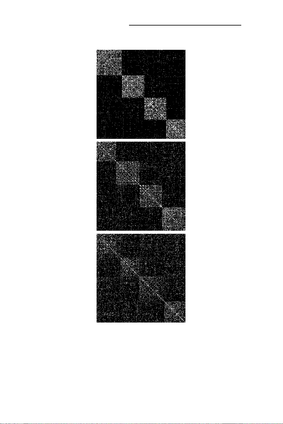
ARENBERG DOCT ORAL SCHOOL F aculty of Engineer ing Cluster ing e v o lving data using k er nel-ba sed methods Rocco Lango ne Disser tation pr esented in par tial fulﬁllment of the req uirements f or the degree of Doctor in Engineerin g J uly 2014 Clustering evolving data using k ernel-based metho ds Ro cco LANGONE Supervisor y Committee: Em. p rof. dr . ir . Paul V an Houtte, chair Prof. dr . ir . Johan A. K. Suykens, promotor Em. p rof. dr . ir . Joos V andew alle Prof. dr . ir . Marc V an Barel Dr . ir . Bart De Ketelaere Prof. dr . Renaud Lambiotte (Université de Namur) Dissertation presented in partial fulﬁllment of the requir ements for the degree of Doctor in Engin eering July 2014 © 2013 KU Leuven – F a culty of Engineering Uitgegeven in eigen b eheer, Rocco La ngone, Kasteelpark Arenb erg 10, B-3001 Heverlee (Belgium) Alle rechten vo o rb ehouden. N i ets uit deze uitgave mag w orden vermenigvuldigd en/of openba ar gemaakt w orden do o r middel van druk, fotok opie, microﬁlm, elektronisch of op we l ke andere wijze o ok zonder vo orafgaande schriftelijk e toestemming van de uitgever. All rights reserved. No part of the publ ication may b e reproduced in an y form by print, photoprint, microﬁlm, electronic or any other means without written p ermission from the pub l isher. ISBN 978-94-6018 - 844-2 D/2014/7515/68 i A mio papá , che mi ha insegnato l’importanza della memoria storica p er capire il pr esente ed immaginare il futur o . A mia mamma , la cu i disarman te semplicitá mi ricor da che i modelli piú semplici e d ele ganti vanno prefer iti a quelli con torti e complicati . Alle mie sor elle Lu isa e Laura, studiose dell’ ”intelligenza natu rale” . A mio fratello Rosario, ”ossessionato” dai r an kings. Preface The work pr esented in this thesis is r elated to th e r esea r ch carried ou t during my do ctoral stu dies at th e ST ADI US (ex SIST A) r esearc h gr oup, inspir ed by the magniﬁcent view of the Ar enb er g castle. It ha s been a priceless time full of enriching experiences both at a pr ofessional and a per son al level. F irst of all, I wish to tha nk my p r omotor Johan Su ykens, who abo ut 4 years ago believed in my abilities and g ave me th e oppo rtunity to start con structing my futur e. During the P hd, h e gave me co ntinuous su pport a nd wa s always pr odig al of suggestions. Many thanks also to the jury members of this thesis, who accepted to r eview the dissertation and pr ovided valuable comments. I would like to acknowledge my actual and former colleagues a nd friends at ESAT for their helpfulness r egar ding work issues, the fr ee time spent together in Leuven, th e spare time enjoyed after nationa l a nd international confer ences. Many thanks to the Erasmus st u dents, vis iting doctoral students and all the friends I met during these years. I will always r emembe r the n ice momen ts shar ed a t the occasion of lunches, dinners, trips, parties etc. Many acknowledgements to my family for cheering me up in difﬁcult time s and sha ring my joy in happy moments. F inally , my most special thanks go to my girlfriend Bruna, w h o ar ound 2 year s ago swept a way th e shadow surr oun ding my heart with love, sweetne ss, and empath y ... iii Abstract Thanks to recent developments of Inform ation T echnologies, ther e is a profusion of av ailab le data in a wide r ange of application do mains ranging from science and engineer ing to bio logy an d business. For this reason, the demand for real-time data pro cessing, mining and analy sis is exper iencing an explo si ve growth in r ecent years. Since labels are usually not av ailab le and in general a full u nderstanding of the data is missing, clusterin g plays a majo r role in shed ding an initial light. In this context, elements such as g eneralization to o ut-of-samp le data, model selection criteria, con sistency of the clu stering results over tim e and scalability to large data become key issues. A su ccessful mod elling fr amew or k is offered by Least Squ ares Suppor t V ector Machine (LS-SVM), which is designed in a primal-d ual optimization setting. The latter allows extension s of the core mo dels b y adding addition al constraints to the primal prob lem, by changing the objecti ve fun ction or by introd ucing new model selection cr iteria. In this th esis, we propo se se veral mo delling strategies to tack le ev o lving data in d if f erent contexts. In the fram e work of static clusterin g, we start by introducin g a soft kernel spectral clu stering (SKSC) algo rithm, which can b etter dea l with overlappin g c lusters with respect to kernel spectral clustering (KSC) and provides mor e interp retable outcom es. Afterwards, a whole strategy based u pon KSC f or commu nity detection of static network s is pro posed, where the extraction of a high quality tra ining sub-gr aph, the cho ice of the kernel fu nction, the mode l selectio n and the applicab ility to large-scale data are key aspects. This paves the way fo r th e development of a novel clu stering algo rithm for the an alysis of evolving networks called kern el spe ctral clustering with memory effect ( MKSC), where the tempo ral smoothn ess between clusterin g results in successive time steps is incorpo rated a t the level of the primal o ptimization prob lem, by pro perly modify ing the KSC form ulation. Later on , an applicatio n of KSC to fault detectio n of an industrial machin e is presented. Her e, a smart pre-p rocessing of the data b y means of a prope r windowing operation is necessary to catch the ongoing degradation p rocess affecting the machine. In this way , in a genuinely unsupe rvised manner , it is possible to ra ise an early warning when n ecessary , in an o nline fashion. Finally , we propose a new alg orithm called increm ental k er nel s p ectral clustering (I KSC) fo r online lear ning v vi ABSTRA CT of no n-stationary data. This ambitiou s ch allenge is faced b y taking a dvantage of the out-of- sample prop erty o f kernel spectr al clu stering (K SC) to adap t the initial model, in order to tack le m erging, splitting or driftin g of c lusters acr oss time. Real- world app lications con sidered in this thesis includ e image segmen tation, time- series clustering, commun ity detection of static and ev olvin g networks. Abb re viations AMS A vera ge Membership S tre ngth ARI Adjusted Rand Index BLF Balanced Line Fit BLF Mem Smoothed Balanced Line Fit Cond Conductan ce Cond Mem Smoothed Condu ctance EF Expansion Factor ESC Evolutionary Spectral Clustering IKSC Incremen tal K ernel Spectral Clustering IKM Incremen tal K-means KKT Karush-Kuhn -T ucker KM K-means KSC Kernel Spectral Clustering LFR Benchmark gr aphs fo r te sting commun ity detection algorithm s LOUV Louvain Method LS-SVM Least Squares Supp ort V ector Machine MKSC Kernel Spectral Clustering with Memo ry effect Mod Modularity Mod Mem Smoothed Modu larity NMI Normalized Mutual Info rmation PCA Principal Compon ent Analysis RBF Radial Basis Function SKSC Soft K er nel Spectral Clustering SC Spectral Clustering SVM Suppor t V ector Machine vii Notation x T T ran spose of a vector x Ω T T ran spose of a matrix Ω Ω ij ij -th entry of the matrix Ω I N N × N I dentity matrix 1 N N × 1 V ector of ones D Tr = { x i } N Tr i =1 T rain ing sample of N Tr data points ϕ ( · ) Fea ture map F Feature space of dimension d h K ( x i , x j ) Kernel function ev aluated on data points x i , x j {A p } k p =1 Partition composed of k clusters α ( l ) i ∈ R i -th entry of the dual solution vector α ( l ) ∈ R N Tr D N × N g raph degree matrix G = ( V , E ) Set of N vertices V = { v i } N i =1 and m edges E o f a graph S = { ( V t , E t ) } T t =1 Sequence of networks over time T | · | Cardinality of a set ix Contents Abstract v Abbre v ia tions vii Notation ix Contents xi 1 Intro duc tion 1 1.1 Backgrou nd . . . . . . . . . . . . . . . . . . . . . . . . . . . . . . . 1 1.2 Challenges . . . . . . . . . . . . . . . . . . . . . . . . . . . . . . . . 2 1.3 Objectives . . . . . . . . . . . . . . . . . . . . . . . . . . . . . . . . 3 1.4 Chapter by Chapter Overview . . . . . . . . . . . . . . . . . . . . . 4 1.5 Main Contributions . . . . . . . . . . . . . . . . . . . . . . . . . . . 6 2 Sp ectral c lustering 9 2.1 Classical Spectral Clustering . . . . . . . . . . . . . . . . . . . . . . 10 2.1.1 Introd uction . . . . . . . . . . . . . . . . . . . . . . . . . . . 10 2.1.2 The Graph Partitioning Problem . . . . . . . . . . . . . . . . 10 2.1.3 Link with Markov Chains . . . . . . . . . . . . . . . . . . . 12 2.1.4 Basic Algorith m . . . . . . . . . . . . . . . . . . . . . . . . 12 xi xii CONTENTS 2.2 Kernel Spectral Clustering . . . . . . . . . . . . . . . . . . . . . . . 13 2.2.1 Generalities . . . . . . . . . . . . . . . . . . . . . . . . . . . 13 2.2.2 Least Squares Supp ort V ector Machine . . . . . . . . . . . . 13 2.2.3 Primal-Dual Formulation . . . . . . . . . . . . . . . . . . . . 15 2.2.4 Model Selection . . . . . . . . . . . . . . . . . . . . . . . . 16 2.2.5 Generalization . . . . . . . . . . . . . . . . . . . . . . . . . 18 2.3 Soft K er nel Spectral Clustering . . . . . . . . . . . . . . . . . . . . . 18 2.3.1 Overview . . . . . . . . . . . . . . . . . . . . . . . . . . . . 18 2.3.2 Algorithm . . . . . . . . . . . . . . . . . . . . . . . . . . . . 20 2.3.3 Model Selection . . . . . . . . . . . . . . . . . . . . . . . . 21 2.3.4 T oy Examp les . . . . . . . . . . . . . . . . . . . . . . . . . . 23 2.3.5 Application: I mage Segmentation . . . . . . . . . . . . . . . 29 2.4 Conclusions . . . . . . . . . . . . . . . . . . . . . . . . . . . . . . . 30 3 Community Detection in Complex Net wo rks 33 3.1 Related work . . . . . . . . . . . . . . . . . . . . . . . . . . . . . . 34 3.2 Methods . . . . . . . . . . . . . . . . . . . . . . . . . . . . . . . . . 36 3.2.1 Representative Sub-grap h Extraction . . . . . . . . . . . . . . 36 3.2.2 Model Selection Criteria . . . . . . . . . . . . . . . . . . . . 38 3.2.3 Choice of the Kernel Function . . . . . . . . . . . . . . . . . 39 3.2.4 Computation al C o mplexity . . . . . . . . . . . . . . . . . . . 40 3.3 Simulations on Synthetic Networks . . . . . . . . . . . . . . . . . . . 41 3.4 Real-W orld App lications . . . . . . . . . . . . . . . . . . . . . . . . 48 3.5 Conclusions . . . . . . . . . . . . . . . . . . . . . . . . . . . . . . . 58 4 Clustering Evo lving Net wo rks 61 4.1 Literature Re v ie w . . . . . . . . . . . . . . . . . . . . . . . . . . . . 62 4.2 The MKSC Model . . . . . . . . . . . . . . . . . . . . . . . . . . . 63 CONTENTS xiii 4.2.1 Cluster Quality Measures in a Dynam ic S cen ario . . . . . . . 66 4.2.2 Computation al C o mplexity . . . . . . . . . . . . . . . . . . . 67 4.3 Framework 1 . . . . . . . . . . . . . . . . . . . . . . . . . . . . . . 67 4.3.1 Artiﬁcial Examp les . . . . . . . . . . . . . . . . . . . . . . . 67 4.3.2 Real-Life Application . . . . . . . . . . . . . . . . . . . . . 76 4.4 Framework 2 . . . . . . . . . . . . . . . . . . . . . . . . . . . . . . 82 4.4.1 Object appe aring and leaving over time . . . . . . . . . . . . 84 4.4.2 T rack ing the clusters . . . . . . . . . . . . . . . . . . . . . . 84 4.4.3 Description of the data sets . . . . . . . . . . . . . . . . . . . 87 4.4.4 Experime nts . . . . . . . . . . . . . . . . . . . . . . . . . . 87 4.4.5 V isualizing the clusters ev olution . . . . . . . . . . . . . . . 94 4.5 Flexibility of MKSC . . . . . . . . . . . . . . . . . . . . . . . . . . 97 4.6 Conclusions . . . . . . . . . . . . . . . . . . . . . . . . . . . . . . . 98 5 Predicting Maintena nce of Industrial Mac hines 101 5.1 Problem Description . . . . . . . . . . . . . . . . . . . . . . . . . . 101 5.2 Materials and Methods . . . . . . . . . . . . . . . . . . . . . . . . . 102 5.3 Results . . . . . . . . . . . . . . . . . . . . . . . . . . . . . . . . . . 103 5.3.1 Hard Clustering . . . . . . . . . . . . . . . . . . . . . . . . . 104 5.3.2 Probabilistic Output . . . . . . . . . . . . . . . . . . . . . . 106 5.4 Comparison with K -mean s . . . . . . . . . . . . . . . . . . . . . . . 108 5.5 Conclusions . . . . . . . . . . . . . . . . . . . . . . . . . . . . . . . 113 6 Clustering No n -Stationary Data 115 6.1 General Overview . . . . . . . . . . . . . . . . . . . . . . . . . . . . 115 6.2 Incremen tal K er nel Spectral Clustering . . . . . . . . . . . . . . . . . 116 6.2.1 Algorithm . . . . . . . . . . . . . . . . . . . . . . . . . . . . 117 6.2.2 Computation al C o mplexity . . . . . . . . . . . . . . . . . . . 119 xiv C ON TENTS 6.3 Synthetic Experimen ts . . . . . . . . . . . . . . . . . . . . . . . . . 120 6.3.1 Description of the data . . . . . . . . . . . . . . . . . . . . . 120 6.3.2 Simulation results . . . . . . . . . . . . . . . . . . . . . . . . 122 6.3.3 Analysis of the eigenvectors . . . . . . . . . . . . . . . . . . 129 6.4 Real-Life Example . . . . . . . . . . . . . . . . . . . . . . . . . . . 130 6.4.1 The PM 10 data-set . . . . . . . . . . . . . . . . . . . . . . . 130 6.4.2 Results of the simulations . . . . . . . . . . . . . . . . . . . 132 6.5 Incremen tal K -mean s Clustering . . . . . . . . . . . . . . . . . . . . 134 6.6 Conclusions . . . . . . . . . . . . . . . . . . . . . . . . . . . . . . . 134 7 Conclusions a nd Future Challenges 139 7.1 General Conclusions . . . . . . . . . . . . . . . . . . . . . . . . . . 139 7.2 Perspectives . . . . . . . . . . . . . . . . . . . . . . . . . . . . . . . 141 A App endix 143 A.1 Cluster Quality Evaluation . . . . . . . . . . . . . . . . . . . . . . . 143 A.1.1 Data Clusterin g . . . . . . . . . . . . . . . . . . . . . . . . . 143 A.1.2 Comm unity Detection . . . . . . . . . . . . . . . . . . . . . 144 A.1.3 Comp aring Partitions . . . . . . . . . . . . . . . . . . . . . . 146 Bibliography 147 Chapter 1 Intro duction 1.1 Background W e live in t h e Information Age. Th e recent de velopm ent of Inform ation T ec hnologies (compu ters, intern et, smart phon es, sensors etc.) has a big impact on science and society . In p rinciple, the large amou nt of av ailab le data can help to grasp the complexity of many phenom ena of inter est, in order to make new scientiﬁc discov eries, designing optimal business strategies, optimizing industrial processes etc. Recognition of complex patterns in the data is of cru cial importan ce to extract usefu l knowledge. In this context, clusterin g is a f undamen tal mode of understand ing and learning [60, 59]. It refers to th e task of organizing the data into meaningful groupings based o nly on the similar ity between the data elements, and th erefore is explorato ry in its essence. Since no target or desired patterns are known a pr iori, it belon gs to the family of unsuperv ised learning technique s [18]. Un veiling the u nderlying struc ture o f the data throu gh the cluster analysis is just one side of the coin. O ther imp ortant elements are related to th e dynam ic version of the p roblem, i. e. m onitoring the evolution of the clusters. Un derstanding how the behaviour of the system un der study chan ges in time re presents a key issue in many domains [103, 50]. From this point of vie w dynamic clustering would be a useful tool to inv estigate how clusters form, e volve and disappear . The topic of this thesis is r elated to th e d esign and application of k ern el-based methods to perf orm dy namic c lustering. Kernel m ethods are a class of machine learning technique s wh ere two main modelling ph ases ar e presen t. First a map ping of the data into a high dimen sional feature space is p erformed . Then , the design o f learning 1 2 INTRODUCTION algorithm s in tha t space allows to discover com plex and non -linear re lations in the original in put space [122]. A major r ole in this work is played by Least Squares Suppor t V ector Machine ( LS-SVM) [128], which is a class of Suppo rt V ector Ma chine (SVM) [ 32] based on a constraine d optimization framework with the p resence o f the L 2 loss function in the ob jecti ve a nd equality instead of inequ ality constrain ts. By modify ing and exten ding the o bjectiv e and/or the constraints of the core f ormulation , it is possible to develop models tailored fo r a given ap plication, with a sy stematic model selection pro cedure and high generalizatio n abilities. 1.2 Challenges The main issues tackled in this thesis can be summar ized as follo ws: • Community detection v ia kernel methods : A network is a collection of nod es or vertices joined by edges and re presents the patter ns o f con nections betwe en the components of complex systems [106]. Usually real-life netw o rks d isplay a high level of o rder and organ ization. For example, the distribution of edges is characterized by high concentratio ns o f edges within special groups of vertices, and low concentrations between these groups. Th e problem of identifying such clusters of nodes is called comm unity detectio n [42]. Th e m ain challenges posed by the usage o f kernel me thods for community d etection are related to the choice of the kernel function, the mo del selection, the out-o f-sample extension, the scalability to large datasets. • Analysis of dynamic co mmunities : Community detec tion of ev olving net- works aims to u nderstand h ow the commun ity structu re of a com plex network changes over tim e [20, 10 3]. A desirable feature of a clustering mode l which has to captur e the evolution of commu nities is the temporal sm oothness b etween clusters in successive ti m e-steps. Providing a consistent clustering at each time results in a smo oth view of the chang es and a greater ro bustness against no ise [27, 25]. • Fault detectio n : W ith the d e velop ment o f in formation and sensor techno logy many p rocess v ar iables in a power plan t like temperatu re, pressure etc. ca n be monitore d. These measurements gi ve an info rmation o n the curr ent status of a machine and can be u sed to pred ict the faults an d plan an optimal maintenanc e strategy [28, 65]. A useful m odel in this case must b e able to catch, in an online fashion, th e degradation process af f ecting the machine , to a void future failure s of the compon ents a nd unplann ed downtimes. • Clustering in a non-stat ionary e n vironment : I n many real-lif e application s non-station ary data are generated accord ing to some distribution models which OBJECTIVES 3 change over time. T herefore, a proper cluster an alysis can be useful to detect importan t chang e poin ts and in general to better under stand the dynamics o f the system und er investigation. I n this case a clustering algo rithm is required to continuo usly adapt in respon se to ne w data an d to be computation ally ef ﬁcient for real-time applications [21]. 1.3 Objectives In this thesis the following objecti ves can be outlined: • to en visa ge a whole kernel-based framework for community detect ion . In this context ma ny issues arise. First o f all it is impo rtant to choo se a p roper kernel fu nction to describe the similarity between the nodes of the network under in vestigation . Then a key point is rep resented by the m odel selection, i.e. ﬁnding the natur al num ber of commu nities which are present in the netw o rk and eventually tun ing the kerne l hyp er-parameters. The kernel-based model must also be able to accurately pr edict the mem bership of n e w nodes jo ining the ne twork, withou t perform ing th e clustering from scratch . Moreover , since many r eal-world networks contain millions of nod es and edg es, th e n etwork data have to be pr ocessed in a reason able tim e. Finally , the research carried out for solving the static commu nity detection prob lem paves the way for the development of mod els for the analysis of e volving networks. • to design a model for co mmunity detection in a changing scenario . An ev olving network can b e describ ed as a sequen ce of snapshot graph s, w here each snapsho t rep resents the con ﬁguration of the network at a particular time instant. When co mmunity d etection is perfo rmed at tim e t , th e c lustering should be similar to the clustering at the p revious time- step t − 1 , and should accurately incorpo rate the actu al d ata. I n this way , if the data at time t doe s no t deviate from historical expectations, the clustering should be similar to that from time t − 1 , while if the structure of th e d ata c hanges s ig niﬁcantly , the clustering must be modiﬁed to account for the new stru cture. Thu s, a good clustering algorithm must tra de-off the beneﬁt o f main taining a co nsistent clusterin g over time with the cost of deviating from an accur ate representation of the curren t data. • to conceive modelling strateg ies f o r clustering stationary and non-statio nary data streams . Da ta stream s are a sequence of d ata recor ds stamped a nd or dered by time [50]. Clustering data streams in real time is an amb itious problem with ample application s. If the data distribution is station ary , emphasis sho uld be giv en to the of f -line construction of the model. On ce prope rly designed, such a model can be u sed to cluster the da ta stream in an online fashion by mean s of the 4 IN TRODUCTION out-of -sample extension. Howev er, if the data distribution is non-stationar y , the initial model soon beco mes obso lete and mu st be quick ly upd ated. There fore the development o f a f ast, adaptiv e and accurate model is an impor tant objec ti ve. 1.4 Chapter b y Chapter Overvi ew The gener al structure of this thesis is sketched in ﬁgure 1. 1 and can be described as follows: • Chapter 2 contain s four sections. First of all a gener al introduction to spe ctral clustering, on e o f the m ost successful clu stering algorithms, is given. Then kernel sp ectral clustering (KSC) is r evie wed. KSC is a spectral clustering algorithm formu lated in the LS- SVM op timization framework, with the possibility to extend the clu stering m odel to out-o f-sample data for predictive purpo ses. Moreover a mo del selection criterion called Balanced Line Fit (BLF) is also pre sent. For these reason s it represents the starting po int to face the challenges d escribed in section 1 .2. L ater on the soft kernel spectra l clustering (SKSC) algorith m is introduced. Instead o f using the hard assignmen t ru le present in KSC, a fuz zy assignment based on the c osine distance from th e cluster pro totypes in the pro jections space is su ggested. W e also introd uce a related mod el selectio n te chnique, called A v er age Membersh ip Streng th criterion (AMS), which solves the major d rawbacks of BLF . Finally , we show that SKSC can improve the interpretability of the results and th e clustering perfor mance with re spect to KSC, mainly in cases of large overlap between the clusters. • Chapter 3 is dedicated to the c ommunity detectio n problem . After reviewing the impo rtant literatu re in the ﬁeld we illu strate our metho dology , which is composed by fo ur m ain corner stones. First, it is crucial to extract f rom the giv en n etwork a small sub- graph representative of its co mmunity structure, which is a challengin g p roblem. This sub- graph can then be used to train a KSC mo del in a comp utationally ef ﬁcien t way and fo rms the basis for a good generalizatio n. Sec ond, the cor rect tu ning of the kernel hyper-parameter s (if any) and the numb er of communities is another importan t issue, which is solved by proposing a new mod el selectio n c riterion based on the Modularity statistics. Third, the kern el functions used to pro perly describe the similarity between the nodes ar e presented. Fin ally , the ou t-of-sample extension allows no t only to accurately pred ict the commu nity afﬁliation of n e w n odes, but also can make the algorithm cluster millions of data in a short time on a desktop computer . • Chapter 4 in troduces a novel model ca lled kernel spectra l clustering with memory ef f ect (MKSC). This meth od is designed to cluster e volving networks CHAPTER BY CHAPTER OVERVIEW 5 (described as a sequen ce of snapshot grap hs), aim ing to track the lon g-term drift of the co mmunities by igno ring meanwhile the short-term ﬂuctuatio ns. In this n e w formulation the de sired temporal smooth ness is incorpo rated in the objective func tion o f the primal p roblem th rough the maxim ization o f the corre lation b etween th e actual an d the previous mode ls. Moreover , new measures are presen ted in order to judge the qu ality of a partitioning pr oduced at a given time. Th e ne w measures are the weigh ted sum of the snapshot quality and the tempor al q uality . The for mer only measur es the quality of the cur rent clustering with r espect to th e cu rrent data, wh ile th e latter measu res the temp oral smoothne ss in terms of th e ab ility of the actu al mod el to c luster the historic data. These new measures can be als o used to perform the model selection. • Chapter 5 discu sses the ap plication of KSC to an industrial case. H ere we assume stationarity , i.e. the regimes experienced by the system unde r analysis do not change over time. V ibration da ta ar e c ollected from a p acking machine to mo nitor its conditions. In order to describe the ongoin g degradation process due to the dir t acc umulation in the sealing jaws we ﬁr st apply a windowing operation on the d ata, accou nting fo r historical values of the sealing quality . The size o f the window , together w ith th e band width of the Radial Basis Fun ction (RBF) kernel and the num ber of cluster s are tuned using the BLF criterion. The n an optima l kernel spectra l clustering model is trained o f ﬂin e to iden tify two main regimes, that we can interpret as normal behaviour and critical conditions (need o f maintenan ce). Thank s to the ou t-of-sample extension prope rty , this model is used onlin e to pred ict in advance when the mach ine need s mainten ance. In princip le, this implies the max imization of th e prod uction capacity and the minimization of downtimes. • Chapter 6 d eals with clu stering n on-stationary data. A new adaptive method named incremental k er nel spectral clustering (IKSC) is devised. In a ﬁrst p hase a KSC model is constructed, then it is u pdated online a ccording to th e new points belo nging to th e data stream. T he central idea beh ind the p roposed technique concern s expressing the clustering mode l in terms of pro totypes in the e igenspace, wh ich are contin uously adap ted throug h th e o ut-of-samp le eigenv ecto rs calculation. M oreover , the trainin g set is forme d only by the c luster centers in the input space, which are als o up dated in re sponse to ne w data. This compact r epresentation of th e model an d the tr aining set in terms of cluster centroids m akes th e metho d comp utationally efﬁcient and allows to prop erly track the ev olution of comp lex patter ns ov er time. • Chapter 7 conc ludes the thesis and proposes future research directions. In gene ral, in all the expe riments discussed in each chapter the values repo rted to assess th e cluster q uality are average measu res over 10 runs o f the algorithm unde r 6 INTRODUCTION Figure 1.1: Thesis overview . in vestigation. Althou gh a fully statistical sign iﬁcance analy sis has not a lw ay s been perfor med, the mean values giv e good in dications abo ut the perfo rmances of the different methods. 1.5 Main Contributions In what follows the main contr ib u tions of this thesis are resumed : • Community detection via KSC . W e co nceived a complete meth odology to cluster network data. The whole pr ocedure ca n b e su mmarized in thr ee m ain stages: extract fro m the network a small s u b-graph which retains the commu nity structure of the en tire g raph, train an op timal KSC model using the selecte d su b- graph as tra ining set, use the out-of-sample extension to assign the memb erships to th e remain ing nod es. The precise tuning o f the hyp er-parameters and the choice of an appropr iate kernel f unction ar e a lso essential. Furth ermore, an algorithm to pr ovide mo derated outputs named SKSC and a related mo del selection criterion called AMS a re proposed. Fin ally we mention how the technique can be used for large scale application s. The relevant papers are [76, 79, 81, 96, 97, 94, 93, 92]. MAIN CONTRIBUTIONS 7 • KSC with memo ry eff ect . A new model is d esigned to handle evolving networks. At the lev el of the pr imal op timization prob lem typical of LS- SVM, we intro duce a memo ry effect in the ob jecti ve functio n to acco unt for the tempor al smo othness of th e clustering results over time. Also new mod el selection criteria spec iﬁc for the giv en app lication are introd uced. The related publication s are [80, 82, 114, 77]. • KSC for predictive maintenance . W e hav e su ccessfully ap plied KSC to a complex industrial case. W e developed a clustering mo del able to infer the degradation process affecting a pac king machine from the vibratio n signals registered b y a ccelerometers plac ed on the sealing jaws. A critical mod elling phase concer ned the windowing of the data in order to d escribe th e h istory of the sealing quality . Mo reover the mo del selection stage was also cr ucial. Finally , to improve the interp retability of the results a probab ilistic output has been provided. This contribution is reported in [78]. • Incremental KSC (IKSC) . W e presented a new algo rithm to perfo rm online clustering in a n on-stationary environment. IKSC exploits the o ut-of-samp le extension p roperty of KSC to continu ously ad apt the initial mo del. In this way it is a ble to c atch the dy namics of the clu sters e volving over time. Th e IKSC metho d can model merging, splitting, appear ance, death, expansio n and shrinking of clusters, in a fast and accurate way [75]. Chapter 2 Sp ectral clustering Spectral clusterin g meth ods have been rep orted to often ou tperform the traditional approa ches such as K -means and hierarch ical clustering in many real- life pro blems. W e start this cha pter with a description of the b asic concepts behind spectral partitioning . W e discuss advantages, like the ability of d etecting comp lex clusterin g bound aries, and d isadvantages, m ainly related to the a bsence o f a model selection scheme and the out-o f-sample e xten sion to unseen data. Then we summar ize the kernel spectral clustering (KSC) m odel, which is for mulated as a weighted k er nel PCA problem in the p rimal-dual optimizatio n f ramew o rk typ ical of Least Squares Support V ector Machines (LS-SVMs). Tha nks to this representation, KSC solves the above mentio ned drawback s of spectral clustering , sinc e it ca n be trained, validated by m eans of a tuning cr iterion called Balanced Line Fit (BLF), and tested in an unsuper vised learning proced ure. Finally we p ropose an algorith m for soft (or fuzzy) c lustering nam ed soft kernel spectral clustering (SKSC). Basically , instead of using the hard assignment m ethod present in KSC, we suggest a fuzzy assignment based on the cosine distance from the cluster proto types in the spac e of the projections. W e also introduce a related model selection techn ique, called average m embership strength (AMS) criterion , which solves the main difﬁculties of BLF . Roughly speaking , SKSC is observed to improve the cluster perfo rmance upon KSC mainly when the clusters overlap to a large extent. 9 10 SPECTRAL CLUSTERING 2.1 Classical Sp ectral Clustering 2.1.1 Intro duction Spectral clustering (SC) r epresents a n elegant and effecti ve solution to the graph partitioning prob lem. It makes u se o f the spectral prop erties o f a matrix repre sentation of the grap h called Laplacian to di vid e it into weakly connected sub-graph s. I t can be applied d irectly to network data to divide the vertices into several n on-overlapping group s, or it can be used to cluster any kind of data. In this case the matrix of pair wise similarities between th e data p oints serves as th e network to partition. I n [29] a n explanation o f SC by th e p oint of view of graph theory is given. Th e au thors of [108] present a SC algo rithm which successfully deals with a numb er of challengin g clustering pro blems. Moreover, an analysis of the algorithm by mea ns of matrix perturb ation theory giv es cond itions under which a good perfo rmance is expected. In [11] a new cost functio n for SC based on a measure of error between a given partition and a solution of the sp ectral relaxation of a minimu m no rmalized cu t p roblem is derived. The authors of [6 3] analyse the SC techniqu e by means of a bi-cr iteria measure to assess the quality of a clustering result. An exhaustive tutorial on SC has been presented in [136]. In what f ollows we on ly dep ict the basic idea behin d spectral partition ing, which or iginated by studying the g raph partitioning problem in graph theory . The interested reade r c an r efer to the afor ementioned works for a deeper discussion. 2.1.2 The Graph P a rtitioning Problem A graph (or network) G = ( V , E ) is a mathematical structure used to mo del pa irwise relations between cer tain ob jects. It r efers to a set of N vertices or n odes V = { v i } N i =1 and a collection o f edg es E that con nect pairs of vertices. If the edg es are provided with weights th e corresp onding g raph is we ighted, otherwise it is r eferred as an u nweighted graph. The topology of a g raph is describ ed by the similarity (o r afﬁnity) matrix, which is an N × N matrix S , wh ere S ij indicates the link between the vertices i an d j . Associated to the similarity m atrix there is the d egree matrix D = d iag ( d ) , with d = [ d 1 , . . . , d N ] T = S 1 N and 1 N indicating the N × 1 vector of ones. Basically the degree d i of node i is the sum of all the edges (or weights) connectin g nod e i with the other vertices: d i = P N j =1 S ij . In the most b asic formulation of the grap h par titioning p roblem one is given an unweighte d gr aph an d asked to split it into k n on-overlapping grou ps A 1 , . . . , A k in order to minimize the cu t size, which is the number of edges ru nning b etween the CLASSICAL SPECTRAL CLUSTERING 11 group s 1 . In order to fa vour balanced clusters, we can consider the normalized cut NC , deﬁned as: NC ( A 1 , . . . , A k ) = k − tr ( G T L n G ) (2.1) where: • L n = I − D − 1 2 S D − 1 2 is called the normalized Laplacian • G = [ g 1 , . . . , g k ] is the matrix co ntaining the n ormalized cluster ind icator vectors g l = D 1 2 f l || D 1 2 f l || 2 • f l , with l = 1 , . . . , k , is the clu ster indicato r vector for th e l -th cluster . I t has a 1 in the entr ies corresp onding to the n odes in the l - th cluster and 0 otherwise. Moreover , the cluster ind icator matrix can be deﬁned as F = [ f 1 , . . . , f k ] ∈ { 0 , 1 } N × k . The NC optimization problem is stated as follows: min G k − tr ( G T L n G ) subject to G T G = I (2.2) with I denoting the id entity matrix. Unfo rtunately this is a NP-h ard prob lem. However we can ﬁnd goo d appro ximate solu tions in polyn omial time by using a relaxatio n method, i.e. a llo win g G to take continu ous values: min ˆ G k − tr ( ˆ G T L n ˆ G ) subject to ˆ G T ˆ G = I . (2.3) with ˆ G ∈ R N × k . In this case it ca n be shown that solving problem (2.3) is equiv alent to ﬁnding the solution to the following eigenv alue problem: L n g = λg . (2.4) Basically , the relaxed clustering infor mation is co ntained in the eigenvectors corre- sponding to th e k smallest eigenv alues of the no rmalized Lap lacian L n . In a ddition to the n ormalized Laplacian , other Laplacians can be deﬁned , like the u nnorm alized Laplacian L = D − S and the rand om walk Laplacian L r w = D − 1 S . T he latter is appealing for its suggestive interpretatio n in ter ms of a Markov ran dom walk. 1 If the graph is weighted, the objecti ve is to ﬁnd a partition of the grap h such that the edges between dif ferent groups hav e very low wei ghts. 12 SPECTRAL CLUSTERING Algorithm 1: SC algorithm [54] Data : positi ve (semi-) deﬁnite similarity matrix S ∈ R N × N , number k of clusters to construct. Result : clusters A 1 , . . . , A k . 1 compute the graph Laplacian ( L , L n or L r w ) 2 compute the eigen vectors ˆ g 1 , . . . , ˆ g k correspondin g t o the smallest k eigen values 3 let ˆ G ∈ R N × k be the matrix containing the vectors ˆ g 1 , . . . , ˆ g k as columns 4 for i = 1 , . . . , N let u i ∈ R k be the vector co rr espond ing to the i -th row of G 5 cluster the points u i into clusters C 1 , . . . , C k 6 compute the ﬁnal partitioning A 1 , . . . , A k , with A i = { j | u j ∈ C i } . 2.1.3 Link with Ma rk ov Chains A well known relationship between graphs and Markov chains exists: any graph has an associated random walk in which the p robability of leaving a vertex is distrib u ted among the outgoin g edges accordin g to their weight. For a gi ven graph with N nod es and m ed ges the probability vector can be deﬁned as p t +1 = P p t , where P = D − 1 S indicates the transition matrix with the ij -th e ntry representin g the proba bility of moving fro m node i to n ode j in on e step. Under th ese assum ptions we have an ergodic and reversible M arkov chain with stationary distribution vector π with com ponents π i = d i 2 m . It can be shown that this distribution describe s the situation in wh ich the random walker remain s mo st of th e time in the same cluster with rar e ju mps to the other clusters [100]. Moreover L r w = I − P and the eigenvectors correspon ding to the smallest eigenv alu es of L r w are the same as the eigenv ec tors r elated to the largest eigenv alues of P : L n g = λg ⇒ ( I − P ) g = λg ⇒ g − P g = λg ⇒ P g = ( I − λI ) g . (2.5) For th e reader intere sted in having a deeper insight in to this topic, we advice to explore [100, 99, 36]. 2.1.4 Basic Algo rithm As mentione d before , the classical sp ectral clusterin g algo rithm can be applied to partition any k ind o f data, not only networks. Indeed , if for the networks we are immediately provid ed with the afﬁnity matrix S , in case of d ata points we have to construct S startin g fro m some similar ity fun ction. The b asic steps are d escribed in algorithm 1. Th anks to the mapp ing of the orig inal input data in the eigenspace, SC is able to unfold the manifold the data are embed ded in and to d etect complex clustering bound aries. On the other hand, it has some clear disadvantages: KERNEL SPECTRAL CLUSTERING 13 • it is not clear how to prop erly construct the similarity matrix S and the number of clusters must be provided beforehan d. In [143] the autho rs pro posed a solution to this model selection issue by introduc ing a parameter-free SC . • there is no clear way as h ow test da ta points should be assigned to the initial clusters, since the emb edding eigenvectors are o nly deﬁned for the f ull dataset. In [138] and [ 44] th e auth ors emp loyed th e Nyström method to ﬁnd approx imate eigen vectors for o ut-of-samp le data an d red uce the com putational load fo r large scale ap plications. In [45] the au thors pro posed a sparse spectral clustering metho d b ased on the incomp lete Cholesky deco mposition ( ICD), which constru cts an ap proxim ation of the Lap lacian in terms of captur ing the structure o f the matrix. By u sing only the in formation related to the piv ots selected by the ICD, a method to compute c luster memberships for out-o f- sample points is also introduce d. 2.2 Kernel Sp ectral Cl ustering 2.2.1 Generalities Kernel Spectral Cluster ing (KSC) rep resents a spectral clu stering form ulation in the LS-SVM optimization framework with primal an d du al repr esentations. The dual problem is an eigenvalue problem , r elated to spe ctral clustering. KSC has two main advantages with respect to classical spectral clustering: • a pr ecise model selection schem e to tune the hy per-parameters • the out-o f-sample e x tension t o test points by means of an underlying model. After ﬁnding the optim al h yper-parameters, th e clustering model can be trained on a subset of the full data and r eadily ap plied to unseen test p oints in a learning fr amew ork . 2.2.2 Least Squa res Supp o rt V ecto r Machine The Suppo rt V ector M achine (SVM) is a state-of- the-art classiﬁcation method. It perfor ms linear classiﬁcation in a h igh-dimen sional kern el-induced feature spac e, which correspo nds to a no n-linear d ecision b oundary in the original input spa ce. LS- SVM differs fro m SVM bec ause it uses a L 2 loss f unction in the primal prob lem and equality instead of inequ ality constraints. This typically leads to eigenv alue problems or lin ear systems at the d ual lev el, in the context o f p rincipal com ponent an alysis [1 29] and classiﬁcation or regression [130], respecti vely . 14 SPECTRAL CLUSTERING Giv en a training data set D Tr = { ( x i , y i ) } N Tr i =1 , where x i ∈ R d are the training po ints and y i ∈ { − 1 , 1 } are th e related labe ls, the primal p roblem of the LS-SVM bina ry classiﬁer 2 can be stated as [130]: min w, e i ,b 1 2 w T w + γ 1 2 N Tr X i =1 e 2 i subject to y i ( w T ϕ ( x i ) + b ) = 1 − e i , i = 1 , . . . , N Tr . (2.6) The expression ˆ y = w T ϕ ( x ) + b indicates the model in the p rimal spa ce. It is linear with respec t to the parameter vector w but the r elationship between x and y can b e non-lin ear if the feature map ϕ ( · ) is a non-lin ear function . With γ we indicate the regularization param eter which contro ls the trade- off between the mode l complexity and the minimization of the training error . If we co nstruct the Lagrangian we hav e: L ( w, e i , b, α i ) = 1 2 w T w + γ 1 2 N Tr X i =1 e 2 i − N Tr X i =1 α i ( y i ( w T ϕ ( x i ) + b ) − 1 + e i ) (2.7) where α i are the Lagrange multipliers. The KKT o ptimality conditions are: ∂ L ∂ w = 0 → w = P N Tr i =1 α i y i ϕ ( x i ) , ∂ L ∂ e i = 0 → α i = γ e i , ∂ L ∂ b = 0 → P N Tr i =1 α i y i = 0 , ∂ L ∂ α i = 0 → y i ( w T ϕ ( x i ) + b ) − 1 + e i = 0 . Eliminating the primal variables e i and w lead s to th e following linear system in the dual prob lem:  Ω + I N Tr /γ y y T 0   α b  =  1 N Tr 0  (2.8) where y = [ y 1 ; . . . ; y N Tr ] , 1 N Tr = [1; . . . ; 1] , α = [ α 1 ; . . . ; α N Tr ] . Th e term Ω m eans the kernel matrix with en tries Ω ij = ϕ ( x i ) T ϕ ( x j ) = K ( x i , x j ) . W ith K : R d × R d → R we denote the kernel fun ction whic h map s the input points into the high dimen sional feature space ϕ ( · ) . For example, by using a Radial Basis Function (RBF) kern el expressed by K ( x i , x j ) = exp( −|| x i − x j || 2 2 /σ 2 ) , one is able to construct a model o f arbitrary comp lexity . Finally , after solv ing the previous linear system, the LS-SVM classiﬁcation mod el in the dual representatio n becomes: y ( x ) = sign ( N Tr X i =1 α i y i K ( x, x i ) + b ) . (2.9) 2 Multi-c lass classiﬁcati on problems are dec omposed into multiple binary cla ss iﬁcat ion tasks with the possibili ty to use se veral coding-decod ing schemes [131]. KERNEL SPECTRAL CLUSTERING 15 The constrained optimization framework with explicit use of regularizatio n exp lained above represen ts the core model not on ly for classiﬁcation, but also regression and unsuper vised learning, as we will see in the remain der of this dissertation. 2.2.3 Primal-Dual F ormul ation Giv en a training data set D Tr = { x i } N Tr i =1 , the multi-cluster KSC model [6] in the LS- SVM framework is for mulated as a weighted kernel P CA p roblem [101] decomposed in l = k − 1 binary prob lems, where k is the num ber of clusters to ﬁ n d: min w ( l ) ,e ( l ) ,b l 1 2 k − 1 X l =1 w ( l ) T w ( l ) − 1 2 N Tr k − 1 X l =1 γ l e ( l ) T V e ( l ) subject to e ( l ) = Φ w ( l ) + b l 1 N Tr . (2.10) The e ( l ) = [ e ( l ) 1 , . . . , e ( l ) N Tr ] T are th e p rojections o f the data points { x i } N Tr i =1 mapped in the feature space along the d irection w ( l ) , also called score variables. The op timization problem (2.1 0) can then be interpreted as the maximization of the weighted v ar iances C l = e ( l ) T V e ( l ) and the contextual minimization of the squared n orm o f the vector w ( l ) , ∀ l . Throug h the regularizatio n c onstants γ l ∈ R + we trad e-off th e mod el complexity expressed b y w ( l ) with th e cor rect represen tation of the trainin g data. V ∈ R N Tr × N Tr is th e weig hting matrix and Φ is the N Tr × d h feature ma trix Φ = [ ϕ ( x 1 ) T ; . . . ; ϕ ( x N Tr ) T ] . The clustering model is expressed by: e ( l ) i = w ( l ) T ϕ ( x i ) + b l , i = 1 , . . . , N Tr (2.11) where as usual ϕ : R d → R d h indicates th e m apping to a high- dimensional featur e space, b l are bias terms, with l = 1 , . . . , k − 1 . The projec tions e ( l ) i represent also the latent v aria bles of the k − 1 binary clu stering in dicators gi ven b y sign ( e ( l ) i ) . T he set o f binary ind icators form a c ode-boo k C B = { c p } k p =1 , whe re each cod e-word is a binary word of length k − 1 represen ting a clu ster . The Lagran gian associated with the prima l prob lem is : L ( w ( l ) , e ( l ) , b l , α ( l ) ) = 1 2 k − 1 X l =1 w ( l ) T w ( l ) − 1 2 N Tr k − 1 X l =1 γ l e ( l ) T V e ( l ) − k − 1 X l =1 α ( l ) T ( e ( l ) − Φ w ( l ) − b l 1 N Tr ) (2.12) where α ( l ) are the Lagrange multipliers. The KKT o ptimality conditions are: 16 SPECTRAL CLUSTERING ∂ L ∂ w ( l ) = 0 → w ( l ) = Φ T α ( l ) , ∂ L ∂ e ( l ) = 0 → α ( l ) = γ l N Tr V e ( l ) , ∂ L ∂ b l = 0 → 1 T N Tr α ( l ) = 0 , ∂ L ∂ α ( l ) = 0 → e ( l ) − Φ w ( l ) − b l 1 N = 0 . Once we have solved the KKT con ditions for op timality , if we set V = D − 1 , we can derive the following du al problem: D − 1 M D Ω α ( l ) = λ l α ( l ) (2.13) where Ω is the kern el matrix with ij -th entry Ω ij = K ( x i , x j ) = ϕ ( x i ) T ϕ ( x j ) . D is the grap h degree matrix wh ich is diago nal with positive elements D ii = P j Ω ij , M D is a centering matrix deﬁned as M D = I N Tr − 1 1 T N Tr D − 1 1 N Tr 1 N Tr 1 T N Tr D − 1 , the α ( l ) are du al variables, λ l = N Tr γ l , K : R d × R d → R is the kernel fun ction. Th e dual representatio n of the mod el becom es: e ( l ) i = N Tr X j =1 K ( x j , x i ) α ( l ) j + b l , j = 1 , . . . , N Tr . (2.14) Moreover , by observing prob lem (2 .13) on e can realize that, apart from the presence of the centering m atrix M D , it is similar to prob lem (2.5). In fact the kerne l matrix plays the role o f the similarity matrix associated to the g raph G = ( V , E ) with v i ∈ V equals to x i . This is also the r eason behin d the choice of the weighting matrix in the primal pro blem as the in verse of the degree matrix D related to the kernel matrix Ω . Finally , the KSC metho d is sketched in alg orithm 2. A visual r epresentation of th e KSC techniq ue is also illustrated in ﬁgure 2.1. 2.2.4 Mo del Selection In gene ral the kernel hyper-parame ters should b e chosen carefully in order to en sure good g eneralization. This is particu larly imp ortant f or very ﬂexible kernels such as the RBF kernel wher e to o sm all values of the band width σ will result in overﬁtting and too high values in a poo r model. T o deal with this cru cial issue, the KSC alg orithm is pr ovided with a m odel selection proced ure based on th e Balanced Line Fit (BLF) criterion [6]. It can b e sho wn that in the ideal situa tion of compact an d well separated clu sters, the points [ e (1) i , . . . , e ( k − 1) i ] , i = 1 , . . . , N Tr , form lines, on e p er each cluster . Then, by exploiting this shape of the points in the projections space , BLF can b e used to select o ptimal clusterin g parameters such as th e number of clusters and e ventually the kernel h yper-parameters. KERNEL SPECTRAL CLUSTERING 17 Algorithm 2: KSC algorithm [6] Data : T raining set D T r = { x i } N Tr i =1 , test set D test = { x test m } N test m =1 kernel func ti on K : R d × R d → R positiv e deﬁnite and localized ( K ( x i , x j ) → 0 if x i and x j belong to differen t clusters), kerne l parameters (if any), number of clusters k . Result : Clusters {A 1 , . . . , A k } , codebook C B = { c p } k p =1 with { c p } ∈ {− 1 , 1 } k − 1 . 1 compute the training eigen vectors α ( l ) , l = 1 , . . . , k − 1 , corresponding to the k − 1 largest eigen v alues of problem (2.13) 2 let A ∈ R N Tr × k − 1 be the matrix containing the vectors α (1) , . . . , α ( k − 1) as columns 3 binarize A and let the code-book C B = { c p } k p =1 be composed by the k encodings of Q = sign ( A ) wi th the most occu rrences 4 ∀ i , i = 1 , . . . , N T r , assign x i to A p ∗ where p ∗ = argmin p d H ( sign ( α i ) , c p ) and d H ( ., . ) is the Hamming distance 5 binarize the test data projections sign ( e ( l ) m ) , m = 1 , . . . , N test , and let sign ( e m ) ∈ {− 1 , 1 } k − 1 be the encoding vector of x test m 6 ∀ m , assign x test m to A p ∗ , where p ∗ = argmin p d H ( sign ( e m ) , c p ) . In particular the BLF is deﬁned in the following w ay : BLF ( D V , k ) = η line ﬁt ( D V , k ) + (1 − η ) balan ce ( D V , k ) (2.15) where D V represents the v alidation set and k a s usual indicates th e n umber o f clu sters. The lineﬁt index eq uals 0 when the score variables are distributed spher ically an d equals 1 wh en the score variables are collinear, represen ting points in the same cluster . The balance index equ als 1 when th e clusters have the same number of elements and tends to 0 in extre mely unbala nced cases. The para meter η co ntrols the importan ce giv en to the line ﬁt with respect to t h e balanc e in dex an d takes values in the range [0 , 1] . Thus, for instance BLF reach es its maximu m value 1 in case of we ll distinct clusters of the same size if η = 0 . 5 . Extensive experiments h a ve shown the u sefulness o f BLF f or model selection. Howe ver , some drawbacks ha ve been observed: • often the criter ion is biased to ward k = 2 clusters • it is not clear how to choose η • it fails in case of large ov er lap b etween the clusters • it is mor e suited for data poin ts than network data. In sections 2. 3 and 3 .2.2 we will show h ow two new mod el selection criteria introdu ced in [ 81] and [76] can solve th ese difﬁculties and th en be used as a valid alternative to BLF . 18 SPECTRAL CLUSTERING 2.2.5 Generalizat ion Spectral clusterin g methods provide a clustering only fo r the given trainin g data without a clear extension to test points, as discussed in [44]. Mor eover , the out-of - sample techn ique pro posed th erein c onsists of applying the Nyström m ethod [12] in order to gi ve an emb edding for the test points by app roximating the under lying eigenfun ction. In [45 ] the information related to the pi vots selected by the I ncomplete Cholesky Decomp osition (ICD) a llo ws to compu te cluster mem berships for ou t-of- sample poin ts. Other similar nu merical tech niques are used in [11 0] and [37] as a solution to using spectral clusterin g for large scale applications. On th e other hand , the extension propo sed in KSC is model-b ased, in th e sense th at the ou t-of-sample points are mapped onto the eigenv ecto rs fo und in the training phase: e ( l ) test = Ω test α ( l ) + b l 1 Ntest (2.16) where Ω test is th e N test × N kernel m atrix ev alua ted using the test points with entries Ω test,ri = K ( x test r , x i ) , r = 1 , . . . , N test , i = 1 , . . . , N Tr . The cluster indic ators can be obtained by binarizin g th e sco re variables. As for the training n odes, the m emberships are assigned by co mparing the se indicato rs with the co de-boo k and selectin g the nearest prototype based on Hamming distance. This scheme co rresponds to an ECOC (Error Correcting Output Codes) decodin g procedure. T o conclude, the LS-SVM f ramew o rk in which KSC h as bee n designed allows to train, validate and test the clustering model i n an unsupervised learning scheme. 2.3 Soft Kernel Sp ectral Cl ustering 2.3.1 Overview Most of the clustering metho ds per forms only hard clusterin g, where each item is assigned to only one group . Howe ver, this works ﬁne wh en the clusters are compact and well separ ated, while the perfo rmance can decrea se dram atically when they overlap. Since this is the case in many real-world scenar ios, soft or fuzzy clustering is becom ing p opular in many ﬁelds [57, 141]. In soft clustering each objec t belongs to se veral gro ups at th e same time, with a different degree of mem bership. Th is is desirable not only to co pe in a more effecti ve way with overlapping clusters, but the uncertainties on data-to-clusters a ssignments h elp also to improve the overall interpretab ility of the results. In what f ollows we describe a novel algorithm for fuzzy clusterin g named soft kernel spectral clusterin g (SKSC) [81]. SKSC is characterized by th e same c ore mod el SOFT KERNEL SPECTRAL CLUSTERING 19 P S f r a g r e p l a c e m e n t s Figure 2 .1: KSC algo rithm . Th e dataset consists o f a set D = { x i } N i =1 where x i ∈ R 2 , and relates to a binary clu stering pro blem with n onlinear b oundary . Af ter binarizing the matrix co ntaining the eigenv ecto rs o f the L aplacian as c olumns, a co de- book with the most frequent binary words representin g th e training cluster prototypes is form ed. The test poin ts are mapped into the training eigenspace through the out-of- sample extension. T hese projection s are then binarized and the p oints are assigned to the closest p rototype in terms of Hammin g distance, by means of an ECOC decoding proced ure. 20 S PECTRAL CLUSTERING as KSC, but it is provided with a different assignmen t rule allowing soft cluster membersh ips. A ﬁr st attem pt to provid e a sort o f p robabilistic o utput in KSC was already d one in [5] . Howe ver, in the cited work the under lying assumptio n is that there is few overlap between the clu sters. On the other hand SKSC can han dle cases where a la rge amoun t of overlap be tween clusters is presen t. Moreover, SKSC uses a new m ethod to tune the numb er of clusters and the kern el hyper-parameters b ased on the soft assignment. This model s elec tion techniqu e is called A v er age Member ship Strength (AMS) criterion. T he latter can s o lve the issues ar ising with BLF mentioned in section 2 .2.4. In fact, unlike BLF , AMS is not biased toward tw o clusters, does not have any parameter to tune and can be used in an ef f ecti ve way also with overlapping clusters. 2.3.2 Algo rithm The main idea behind soft kern el spectral clustering is to use KSC as an initializatio n step in o rder to ﬁnd a ﬁr st division of the training data into clusters. Then this gro uping is reﬁned by re-calcu lating the prototypes in the score v ariab les space, and the cluster assignments are perfor med by m eans of the cosine distance between each po int and the proto types. This allows also to ob tain highly sparse models as explained in [91], where a possible alternative to reduced set methods (see [95]) is proposed. As already pointed o ut in section 2.2.4 , in the pr ojections/score variables space the points belong ing to the same cluster appear aligned in the absen ce of overlap ( see center of Fig ure 2.2). In this ideal situation of clear and well d istinct group ings, any soft assignment shou ld reduce to a hard assignment, where every point must belong to one cluster with member ship 1 and to th e other clusters with member ship 0 . In fact, th e membership reﬂects the certainty with which we can assign a poin t to a cluster and it can be though t as a kind of subje cti ve pro bability . In ord er to cope with this situa tion, th e co sine distance from every po int to the pro totypes can be used as the basis fo r the soft assignme nt. In this way , in the perf ect above- mentioned scenario, every point position ed along on e line will be assigned to that cluster with mem bership or probability equ al to 1 , since the cosine distanc e fro m the correspo nding pr ototype is 0 , bein g the two vectors parallel ( see bottom of Figure 2 .2). Giv en the projection s for the training p oints e i = [ e (1) i , . . . , e ( k − 1) i ] , i = 1 , . . . , N Tr and the corr esponding hard assignments q p i we can calculate for each cluster the new prototy pes s 1 , . . . , s p , . . . , s k , s p ∈ R k − 1 as: s p = 1 n p n p X i =1 e i (2.17) where n p is the number o f points assigned to cluster p durin g the initialization step by KSC. Th en we can calculate the cosine distance between the i -th poin t in th e score SOFT KERNEL SPECTRAL CLUSTERING 21 Algorithm 3: SKSC algorithm [81] Data : T raining set D T r = { x i } N Tr i =1 and test set D test = { x test m } N test m =1 , kern el function K : R d × R d → R positiv e deﬁnite and localized ( K ( x i , x j ) → 0 if x i and x j belong to differen t clusters), kerne l parameters (if any), number of clusters k . Result : Clusters {A 1 , . . . , A p , . . . , A k } , soft cluster memberships cm ( p ) , p = 1 , . . . , k , cluster prototypes S P = { s p } k p =1 , s p ∈ R k − 1 . 1 Initialization by solving eq. (2.14). 2 Compute the ne w prototypes s 1 , . . . , s k (eq. (2.17)). 3 Calculate the test data projections e ( l ) m , m = 1 , . . . , N test , l = 1 , . . . , k − 1 . 4 Find the cosine distance b etween each projection and all the prototypes (eq. (2.18)) ∀ m , assign x test m to cluster A p with membership cm ( p ) according to eq. (2.19). variables space and a prototype s p using the following formula: d cos ip = 1 − e T i s p / ( || e i || 2 || s p || 2 ) . (2.18) The membersh ip o f point i to cluster q can be expressed as : cm ( q ) i = Q j 6 = q d cos ij P k p =1 Q j 6 = p d cos ij (2.19) with P k p =1 cm ( p ) i = 1 . As discussed in [1 4], this membership is gi ven as a subjectiv e probab ility and it indicates the strength of belief in the clustering assignment. The out-of -sample extension on unseen data consists of two steps: 1. proje ct the test points on to the eigenspace spanned by [ α (1) , . . . , α ( k − 1) ] using eq. ( 2.16) 2. calculate the cosine distanc e between these p rojections an d the training cluster prototy pes, a nd then the correspon ding soft a ssignment by means of eq. (2.19 ). The SKSC method is summariz ed in alg orithm 3. T he main steps of this techn ique are depicte d in ﬁgure 2.3. 2.3.3 Mo del Selection From the soft assignmen t techniqu e exp lained in the previous section a new model selection method can be derived. In fact, we can calculate a kind o f mean membership per cluster indicating the a verage degree of belon ging of the points to that cluster . If 22 S PECTRAL CLUSTERING −4 −3 −2 −1 0 1 2 3 4 −4 −3 −2 −1 0 1 2 3 4 P S f r a g r e p l a c e m e n t s −0.2 −0.1 0 0.1 0.2 0.3 0.4 0.5 −0.4 −0.3 −0.2 −0.1 0 0.1 0.2 0.3 P S f r a g r e p l a c e m e n t s e (1) e (2) P S f r a g r e p l a c e m e n t s e ( 1 ) e ( 2 ) Figure 2.2: Clusters as lines in the e ( l ) space : example of ho w three distinct clusters ( 3 conce ntric ring s on the top in a 2D spa ce) appear in the p rojection space in the KSC formu lation (center). On the botto m an illustration of the cosine distance in the scor e variable space is gi ven: the j -th point is parallel to the prototy pe so its member ship is 1 . Th is is not the case for the i -th point. SOFT KERNEL SPECTRAL CLUSTERING 23 Algorithm 4: AMS mod el selection algorith m for SKSC [81] Data : training and v alidation sets, kernel function K : R d × R d → R positive d eﬁnit e and localized. Result : selected number of clusters k , kernel parameters (if any). 1 Deﬁne a grid of va lues for the parameters to select 2 T rain the related SKS C model using the training set 3 Compute the soft cluster assignments for the points of the validation se t 4 For e very partition calculate the related AMS score using eq. (2.20) 5 Choose the model with the highest score. we do th e same for every cluster and we take the mean, we h a ve what we call the A vera ge Membership S tre ngth (AMS) criterion 3 : AMS = 1 k k X p =1 1 n p n p X i =1 cm ( p ) i . (2.20) For k = 2 the Eu clidean distanc e b etween th e po ints and the p rototypes is used 4 , while fo r k > 2 we consid er the cosine distance. Unlike BLF , AMS do es no t have any parameter to tune, it is not b iased tow ar d k = 2 and as we will show in the experimental section it can be used in an effecti ve way a lso in c ase of overlapping clusters. The model selection proced ure is d escribed in algorithm 4. 2.3.4 T o y Examples In th is section some experime ntal example s with artiﬁcial data are presented to illustrate the pro posed soft clusterin g techniqu e. W e comp are SKSC with KSC in terms of Adjusted Rand Index (ARI) [5 8], me an Silhou ette value (MSV) [ 119] and Davies-Bouldin index ( DBI) [34] (see appendix 5 ), and AMS with BLF . In genera l we observe that SKSC achieves better results tha n KSC and the AMS c riterion appears to be mo re useful than BLF for model selection , mostly when a big amo unt of overlap between clusters is present. W e ha ve designed a n experimen t with the goal o f un derstanding the role o f the ov er lap rather than the no nlinearities to affect the clustering perform ances. T hus, synthetic data co nsisting of 1000 d ata points h a ve be en generated from a mixtur e of three 2D Gaussians, with 5 00 samples drawn fro m each compo nent of the mix ture. W e then 3 Future work can be relat ed to experiment with a weighted ver sion of the AMS criterion. T he weights could be chosen, for inst ance, to emphasize the contrib ution of poi nts with highest membership, in order t o reduce the inﬂuence of the noise. 4 In this case the cosine distan ce is not discrimin ativ e because the points lie on a line. 5 A summary of the main cluste r qualit y measures used in this thesis will be gi ven in the appendix. 24 S PECTRAL CLUSTERING P S f r a g r e p l a c e m e n t s Figure 2.3 : SKSC algo rithm . Th e dataset consists o f a set D = { x i } N i =1 where x i ∈ R 2 , and relates to a binary clustering pr oblem with nonline ar boundary . From the projectio ns of the training points in the eigenspace of th e Laplacian som e cluster prototy pes ar e comp uted. The pr ojection of the test po ints are the n assigned to the different clusters with a prob ability dep ending on th e cosine distance fro m e ach o f them. SOFT KERNEL SPECTRAL CLUSTERING 25 consider d if f erent am ounts of overlap between these clouds of po ints, as d epicted in ﬁgure 2.4 from top to bottom . In ﬁgur e 2.5 we show the model selection plots fo r these three cases. W e can see th at AMS, even in case of large overlap, is able to correc tly identify the p resence of the three distinct Gau ssian clouds. Th is is not the case f or the B LF criterio n. In tables 2.1, 2.2, 2.3 the c lustering results of KSC and SKSC (when fed with correct p arameters) are evaluated. W e can notice that SKSC ou tperform s KSC w hen the overlap between the clu sters increases. Fina lly , in ﬁg ure 2.6 the soft clu stering results prod uced b y SKSC fo r the large overlap case ar e depicted. As we would expect, the pro bability to belong to each of the 3 clusters decreases in the overlapping regions. KSC SKSC MSV 0 . 96 0 . 96 DBI 0 . 2 4 0 . 24 ARI 1 1 T able 2 .1: Three G aussians, no overlap : clu ster quality ev alu ation of KSC and SKSC based on Mean Silhoue tte V alue (MSV), Davies-Bouldin I ndex (DBI) , and Adjusted Rand Index ( ARI). A summary of these an d oth ers cluster q uality criteria is given in the Appen dix. KSC SKSC MSV 0 . 90 0 . 91 DBI 0 . 3 4 0 . 33 ARI 0 . 96 0 . 99 T able 2.2: T hree Ga ussians, few overlap : clu stering results of KSC and SKSC accordin g to Mean Silhouette V alue, Davies-Bouldin Index, and Adjusted Rand Ind ex (see Appen dix). The best perform ances are in bold. KSC SKSC MSV 0 . 59 0 . 64 DBI 0 . 7 9 0 . 76 ARI 0 . 65 0 . 74 T able 2.3: Three Gaussians, la rge overlap : cluster quality mea sures (see Appen dix) for KSC and SKSC, with the best perfo rmance in bold . 26 S PECTRAL CLUSTERING −20 −15 −10 −5 0 5 10 15 20 −20 −15 −10 −5 0 5 10 15 20 P S f r a g r e p l a c e m e n t s No Overlap −15 −10 −5 0 5 10 15 −15 −10 −5 0 5 10 15 P S f r a g r e p l a c e m e n t s Few Ov er lap −15 −10 −5 0 5 10 −10 −8 −6 −4 −2 0 2 4 6 8 10 P S f r a g r e p l a c e m e n t s Large Overlap Figure 2.4: Three G aussians dat aset . The dataset consists of three sets of N poin ts in a 2 D space ( x i ∈ R 2 , i = 1 , . . . , N ) representing Gaussian m ixtures with different amount of overlap. SOFT KERNEL SPECTRAL CLUSTERING 27 2 3 4 5 6 7 8 9 10 0.65 0.7 0.75 0.8 0.85 0.9 0.95 1 AMS BLF P S f r a g r e p l a c e m e n t s Number of clusters k No Overlap 2 3 4 5 6 7 8 9 10 0.65 0.7 0.75 0.8 0.85 0.9 0.95 1 AMS BLF P S f r a g r e p l a c e m e n t s Number of clusters k Few Ov er lap 2 3 4 5 6 7 8 9 10 0.4 0.5 0.6 0.7 0.8 0.9 1 AMS BLF P S f r a g r e p l a c e m e n t s Number of clusters k Large Overlap Figure 2.5 : Model selection for the three Gaussians dataset . The tru e n umber of clusters is k = 3 . T wo model selection criteria, namely AMS and BLF , are contrasted . W e c an notice how th e former can better deal with overlapping clusters. 28 S PECTRAL CLUSTERING 0.1 0.1 0.1 0.1 0.1 0.1 0.1 0.2 0.2 0.2 0.2 0.2 0.2 0.2 0.3 0.3 0 .3 0.3 0.3 0.3 0.3 0.4 0 .4 0.4 0.4 0.4 0.4 0.5 0.5 0.5 0.5 0.5 0.6 0 . 6 0.6 0.6 0.6 0.7 0 . 7 0.7 0.7 0.7 0.8 0 . 8 0.8 0.8 0.8 0.9 0 . 9 0.9 0.9 0.9 0.1 0.1 0.4 0.4 0.5 0.5 0.5 −20 −15 −10 −5 0 5 10 15 −20 −15 −10 −5 0 5 10 15 0.1 0.2 0.3 0.4 0.5 0.6 0.7 0.8 0.9 P S f r a g r e p l a c e m e n t s p 1 0.1 0.1 0.1 0.1 0.1 0 . 1 0.1 0.1 0.1 0.1 0.2 0.2 0.2 0.2 0.2 0.2 0.2 0.2 0.3 0.3 0.3 0.3 0.3 0.4 0.4 0.4 0.4 0.4 0.5 0.5 0.5 0.5 0.5 0.6 0.6 0.6 0.6 0.6 0.7 0.7 0.7 0.7 0.7 0.8 0.8 0.8 0.8 0.9 0.9 0.9 0.9 0.1 0.1 0.1 0.2 0.2 0.1 0.1 0.3 0.2 0.3 0.1 0.4 −20 −15 −10 −5 0 5 10 15 −20 −15 −10 −5 0 5 10 15 0.1 0.2 0.3 0.4 0.5 0.6 0.7 0.8 0.9 P S f r a g r e p l a c e m e n t s p 2 0.1 0.1 0.1 0.1 0.1 0.1 0.2 0.2 0.2 0. 2 0.2 0.3 0.3 0.3 0.3 0.3 0.4 0.4 0.4 0.4 0.4 0.5 0.5 0.5 0.5 0.5 0.6 0.6 0.6 0.6 0.7 0.7 0.7 0.7 0.8 0.8 0.8 0.8 0.9 0.9 0 .9 0.9 0.1 0.1 0.1 0.1 0.1 0.1 0.1 0.1 0.1 0.1 0.1 0.1 −20 −15 −10 −5 0 5 10 15 −20 −15 −10 −5 0 5 10 15 0.1 0.2 0.3 0.4 0.5 0.6 0.7 0.8 0.9 P S f r a g r e p l a c e m e n t s p 3 Figure 2. 6: Sof t clustering res ults for three Gaussians dataset with large overlap : probab ility to belong to clu ster 1 ( p 1 , to p), to cluster 2 ( p 2 , center) and to cluster 3 ( p 3 , bo ttom) d etected b y SKSC for the large overlap ca se. W e can no tice that all the probab ilities reach their maximum value ar ound the centroids and then dec rease in the overlapping region. SOFT KERNEL SPECTRAL CLUSTERING 29 2.3.5 Application: Image Segmentation Here we show the usage o f SKSC fo r the ima ge segmentation task. I n compu ter vision, image segmentatio n is the process of partition ing a digital image into multiple sets o f pixels, such that pixels in the same grou p share certain visual character istics. W e random ly selected 10 color images from the Ber keley image dataset [98]. Before clustering the images, a pr e-processing of the data was ne cessary . In particula r , we computed a loca l co lor histogram with a 5 × 5 pixels wind ow aroun d each pixel using minimum variance colo r quan tization of 8 levels. Then , in orde r to compar e the similarity between two histogra ms h ( i ) and h ( j ) , the po siti ve de ﬁnite χ 2 kernel K ( h ( i ) , h ( j ) ) = exp( − χ 2 ij σ 2 χ ) h as been adopted [44]. The symbol χ 2 ij denotes the χ 2 ij statistical test used to compar e two proba bility distributions [1 15], σ χ as usual indicates the band width of the kernel. A randomly selected s u bset of 1000 pixels forms the trainin g set and the wh ole image is the test set, in order to o btain the ﬁnal segmentation. After p roperly selectin g the num ber of cluster s an d the kern el b andwidth fo r each im age, we compar ed the segmentation obtained by KSC and SKSC by using three e valuation measures [8]: • F-measur e ( 2 · P r ecision · Recall P r ecision + Recall ) with respect to human ground- truth b oundar ies • V ariation of inform ation (VI): it measures the distance between two segmenta- tions in terms of their average co nditional en tropy . Low values indicate good match between the segmentations. • Prob abilistic Rand I ndex (PRI): it operates b y co mparing the con gruity of assignments between pairs o f ele ments in the clusters f ound by an algorithm and multiple groun d-truth segmentations. The segmentation results ar e shown in ﬁgure 2.7 (F-measur e) and tab les 2.4 (VI) and 2.5 (PRI). For compar ison purpo ses, the soft partitio ning obtaine d b y SKSC is transform ed in hard clu stering results by assigning the pixels to the closest pro totype. In this case th e perfo rmances o f SKSC and KSC ar e overall similar, mo st probab ly due to the fact that the imag es are character ized by clear segments (i.e . small overlap). Finally , in ﬁgur e 2 .8 the segmen tations acco mplished by SKSC o n three selected images are depic ted for illustration purp ose. 30 S PECTRAL CLUSTERING 2.4 Conclusions In this chapter, after introd ucing th e basics of spectral partitioning, we have d iscussed the LS-SVM m odelling fr amew or k and we sum marized the KSC algorith m. Th e latter is a spectral clustering mod el formu lated as weigh ted kern el PCA in a primal-d ual optimization setting. Th is fo rmulation allows a simple extension of the mode l to out-of -sample p oints a nd a systematic model selection p rocedure based o n th e BLF criterion. Then, we presented the soft kernel spectral clustering ( SKSC) technique, which is based on KSC but it uses a fuzzy assignmen t rule. The latter dep ends on the cosine distance of e very poin t from the cluster pro totypes in th e projection s space. A new model selection techniqu e d eriv ed from this soft assignment, namely the a verage membersh ip strength (AMS) criterion, is also p roposed. W e showed how AMS solves the main drawbacks of BLF and can be u sed more ef f ecti vely in presence o f overlap between clusters. W e illustrated on toy data and an image s egmen tation problem, that SKSC outperfo rms KSC mainly in the most dif ﬁcu lt tasks (i. e. when clusters overlap to a large extent). Mo reover , SKSC pr oduces mo re interpr etable results d ue to its fuzzy natur e. 0 0.1 0.2 0.3 0.4 0.5 0.6 0.7 0.8 0.9 1 0 0.1 0.2 0.3 0.4 0.5 0.6 0.7 0.8 0.9 1 Recall Precision P S f r a g r e p l a c e m e n t s Figure 2.7: F-measure plot : ev alua tion of KSC (red) and SKSC (b lue) algo rithms with respec t to human bou ndaries in th e image segmentatio n task. Iso-F curves are shown in green. The green do t indicates the average agreement be tween the human subjects who perfor med the segmentations used as ground -truth. CONCLUSIONS 31 Image ID KSC SKSC 14508 6 3 . 11 3 . 10 42049 3 . 42 3 . 41 16706 2 1 . 84 1 . 69 14709 1 1 . 10 1 . 10 19607 3 0 . 18 0 . 18 62096 0 . 35 0 . 31 10108 5 2 . 77 2 . 69 69015 2 . 36 2 . 36 11908 2 0 . 90 0 . 89 3096 2 . 97 2 . 97 T able 2.4 : VI crit erion : comparison of KSC and SKSC segmentations in terms of variation of in formation (th e lower the better). Best performa nce in bo ld. The algorithm s have a similar perfor mance. Image ID KSC SKSC 14508 6 0 . 59 0 . 59 42049 0 . 70 0 . 71 16706 2 0 . 83 0 . 7 7 14709 1 0 . 83 0 . 83 19607 3 0 . 98 0 . 98 62096 0 . 95 0 . 9 4 10108 5 0 . 37 0 . 38 69015 0 . 58 0 . 58 11908 2 0 . 87 0 . 87 3096 0 . 19 0 . 19 T able 2.5: PRI criter ion : co mparison of KSC a nd SKSC segmentation s in ter ms of probab ilistic rand ind ex (the higher the better). Best perfo rmance in bo ld. In ge neral, the metho ds produce a similar outcom e. 32 S PECTRAL CLUSTERING P S f r a g r e p l a c e m e n t s P S f r a g r e p l a c e m e n t s P S f r a g r e p l a c e m e n t s P S f r a g r e p l a c e m e n t s P S f r a g r e p l a c e m e n t s P S f r a g r e p l a c e m e n t s Figure 2.8: SKSC seg mentations : origin al imag es (lef t) an d SKSC segmentatio ns (right) for image IDs 6901 5 , 1470 9 1 , 1960 73 . Chapter 3 Communit y De tection in Complex Net w o rks Community de tection ref ers to the prob lem o f p artitioning a complex network into clusters of nod es with high d ensity of edges, in order to und erstand its structure and fun ction. A pro fusion of alg orithms has been p roposed in the recent past since many real-world a pplications arise in different ﬁelds, from biolo gy to computatio nal social sciences. In this chap ter we propo se a who le kernel- based framework for commun ity d etection. T he ma in steps of ou r appro ach are the extractio n o f a sub- graph rep resentativ e of the comm unity structure of the entire network fo r training the clustering mode l, th e validation stage by means o f pro per mod el selection criteria, and the memb ership assign ments for th e rema inder o f the n odes via o ut-of-samp le extension. In contrast to most of th e method s pr esent in the literatu re which are rather speciﬁc, our techn ique is m ore ﬂexible b ecause in the model selection phase the user can provide the desired criterio n, in o rder to obtain a ﬁnal partition ing with cer tain characteristics. Moreover , th e out- of-sample extension allows to rea dily assign the membersh ip to n e w nodes join ing the network without u sing h euristics. Also we c an deal wi th weighted and unweigh ted networks by choosing the suitab le kernel function , and gr aphs with overlappin g c ommunities can be analysed. Fina lly , by exploiting the high sparsity of the majority of the real graphs, the method can scale to large network data even on a desktop computer and can be easily parallelized. 33 34 COMMUNITY DETECTION IN COMPLEX NETWORKS 3.1 Related w o rk In nature, science and technology complex systems are usu ally organized in networks of intera ctions b etween many com ponents. Although ev er y system ha s its peculiar proper ties, a commo n architec ture can be r ecognized [ 123]. It seem s that c omplex networks are organized in modules or commu nities, and this feature can be explained by con sidering two im portant aspects: re silience and adap tation. Man y studies suggested th at if a pa rt of a complex system stops work ing p roperly , the mo dular organization allows to circu mvent the pro blem, making it more resilient to failures. Moreover , the com munity structure helps such a system to a dapt quickly to chang es in the environment [ 31]. A network (or graph) with N no des is ch aracterized b y a community structure wh en group s o f nodes for ming tightly conn ected u nits are on ly weakly linked to each other . Un covering the natural communities present in a complex network has recently become a major top ic in science and enginee ring with an in terdisciplinary effort [42, 106, 30, 9, 116]. This interest is d ue to th e fact that r e vealing the m odular struc ture of a network can be very u seful for a number o f reason s like visualizing large graphs composed of millions of nod es and edges, in vestigating the f unction o f each mo dule, discovering the role of the different nodes inside a community . Many alg orithms to handle the com munity d etection p roblem h av e been pro posed, with different character istics. Th e most popular algorithm is tha t introdu ced in [ 47]. The method is h istorically im portant b ecause it pop ularized comm unity detection among physicists and engineers and fa voured t h e search of ne w algorithm ic solu tions. It is b ased on the removal of edges with high betweenne ss, which expresses the participation of an edg e to th e inf ormation ﬂo w on a gr aph. The co nnected compon ents of the remainin g network are the commu nities d etected by th e m ethod. Even if q uite appea ling the algor ithm is slow (it scales a s O ( N 3 ) ) an d c annot d eal with overlapping co mmunities, as each vertex is assigned to a single cluster . A large n umber o f su ccessful techniques is based o n M odularity m aximization, whic h describes the streng th of th e com munity structur e by comparing the actual g raph with a rando m graph sharing the same degree distribution [105]. A well-kn own algorithm (with linear run-tim e O ( N ) ) is the Louv ain method [19], based on a gre edy optimization of the Mod ularity . The Mod ularity maxima found by the meth od are also better than those fo und with anoth er well-known greed y technique used in [30]. The most pop ular algorith m for discovering overlapping comm unities is the Clique Percolation Method (CPM) [11 2], which is based on the idea that node s inside a commun ity are likely to form cliques, in contrast to inter-community edges. Ano ther recent and very fast tech nique for overlapping commu nity detection is [140], built on a n ovel a nd co unter-current observation that in many n etworks overlaps between commun ities are den sely connected and can reveal th e mod ules. In [ 41] the author s use a p artition of the links o f a n etwork (instead of clustering the no des) to uncover its RELA TED WORK 35 commun ity structu re. In th is way their meth od can better d etect no des belongin g to m ore than one commu nity . A d ifferent class of meth ods are th ose based on informa tion-theore tic ideas, such as the minim um-descrip tion-length meth od called Infom ap intr oduced in [118]. All th e a bove-mentioned algorithm s can discover clusters at a particular scale, and ev en if they pr oduce hierarch ical results the re is no guaran tee th at the relev ant partitions ar e no t ar tefacts. On the oth er han d multi- resolution techniques able to ide ntify t h e dif feren t levels o f organization of vertices in clusters have b een prop osed. They ar e inspired by different principles. For example in [1 17] and [9] the authors use different deﬁnitions of Modularity and the Laplac ian matrix respectively , th e algor ithm introduced in [36] is developed on the stability o f clustering under rand om walk, in [72] a ﬁtness function which estimates the strength of a cluster and entails a resolution param eter is optimized. In this co ntext, also spectra l alg orithms p lay an im portant ro le. Although most spectral methods h a ve been focused on data clusterin g, many applications to n etwork data for commun ity detection exist [38, 61, 24]. As for data clustering s o me iss u es arise when using spectral clustering for commu nity detection: • the co nstruction and stora ge of th e N × N adjacen cy m atrix de scribing the g raph becomes infeasible for large networks • the com putation of the eigenv ecto rs of the La placian is comp utationally expensiv e O ( N 3 ), althou gh some appro ximation techniqu es like the Lanczos method [74], the Nyströ m algorithm [44] an d the power iteration method [8 7] can speed-up the process • it is not clear h ow to choose the nu mber of co mmunities into which to split the network at hand • it does not incorp orate a clear extension to o ut-of-sam ple nodes. Howev er, numerical techn iques like the Nyström metho d [44], or incremental algorith ms like [1 10, 37] provide a possible way to tackle this iss u e. Recently , also a spar se spectral clu stering meth od based on the Inc omplete Cholesky Dec omposition (ICD) g i ves the possibility to perfo rm out-o f-sample extension b y exploitin g the pivots selected b y the ICD [45]. B eside s spectral clu stering, most of the algor ithms for c ommunity detection work only at th e training lev el. They prod uce a partition o f the n etwork into mod ules but cann ot assign th e membersh ip to new nod es join ing th e n etwork withou t ru nning fr om the beginning or using heuristics. In the comm unity detection ﬁeld, to the best o f our knowledge the only kind of alg orithm providing a systematic out- of-sample extension to test n odes are those on e based on statistical inference by means o f block models [125, 111, 3]. 36 COMMUNITY DETECTION IN COMPLEX NETWORKS In what follows we describe a method ology that casts the c ommunity detection problem in a mach ine learning algorith m. Our core model is KSC [ 6], wh ich ha s been summar ized in the previous chap ter . In th is way we are able to handle the aforemen tioned issues in a unique f ramew o rk, and to propo se a competitive techniqu e for the analysis of complex networks. Moreover, this work p a ves the way to th e development of the MKSC mod el for the a nalysis of ev o lving n etworks discussed in chapter 4. 3.2 Metho ds The usage of KSC for comm unity detection can be summarize d in three main stages: • subset extraction : in or der to solve an affordable eigenv alue prob lem for training the mod el, we n eed to select a subset o f th e entire network that captu res th e inherent commu nity structure 1 • mod el selection: th e pr oper number of commun ities an d the kernel hyper- parameters must be tuned carefully to ensure good results • out- of-sample extension: once con structed an optimal mo del, the memberships for the remaind er o f the network can be ass ig ned via eq. (2 .16). Furthermo re, the choice of an appro priate kernel function which depicts the similarity between the nodes is very important. 3.2.1 Rep resentative Sub-graph Extraction Sampling a sub- graph represen tati ve of the comm unity structur e of the who le network under stud y is a cr ucial task in our fra mew ork , since it a llo ws a m eaningfu l out-o f- sample extension to nod es no t present in the training set. Simp ly tak ing a rando m sample o f no des can lead to very different results in sev er al run s, since the qua lity of the selected sub-grap h can have a huge variability . Also selecting a sub set in such a way that it follo ws the same degree distrib ution or between ness centrality distribution of the wh ole graph can produce samples that ar e not rep resentativ e of the c ommunity structure of the larger network. Recen tly , a new q uality function describin g th e representativeness of the sam ple with r espect to the community structure o f the whole 1 Ho w to choose such a subgraph is an open proble m . In general it is selec ted by e xperimental e va luation, where one wants to ﬁnd a trade-of f between a sm all size (to reduce the computati onal bu rden) and a good qualit y of the c lustering results on the ent ire network (which depend s on how well the subset repre sents the community structure of the whole graph). METHODS 37 graph has been introd uced in [90]. This qu ality fun ction is called Expan sion Factor (EF) a nd is deﬁn ed as | N ( A G ) | |A G | , where A G indicates a subset of the graph G , N ( A G ) its neighb ourho od, i.e. the remainin g pa rt of the network to which A G is conn ected, and | · | den otes the cardin ality of a set. The idea is th at b y selecting a sub-g raph for which the expansion factor is maxim um, o ne samples a r epresentative subset. Rou ghly speaking, b y inclu ding in A G nodes that be st con tribute to the expan sion factor , we are taking nodes th at are more connected to the rest of th e netw o rk than to A G . The se nodes are then very likely to belong to clusters no t yet rep resented in the sub-g raph, allowing us to produ ce a samp le which is a cond ensed representation of the co mmunity structure of the whole network. In [79] we p roposed a g reedy strategy for the optimization of EF , which can be summarized in alg orithm 5. Th e selection of the active sub set can take from a few to sev er al minutes or ho urs depen ding o n the size N of the entire network and its sparsity , the cho sen size N A for the active subset and the thre shold ǫ . Moreover , although the variability of the method is less compar ed to the r andom sampling , the technique is stochastic by nature. In [94] the Fast and Uniq ue Repr esentativ e Subset (FURS) selection technique has been proposed to cope with these issues. Th e method has been shown to be computatio nally less expensive and determin istic: it greed ily selects nodes with high- degree centrality fro m mo st or all th e m odules pre sent in the network, which a re usually located at the center rather than the periph ery and can better capture the comm unity st r ucture. Algorithm 5: EF-based subset selection [79] Data : network G = ( V , E ) composed of N nodes V = { n i } N i =1 (represented as the adjacenc y matrix A ∈ R N × N ), N A (size of sub-grap h A G ). Result : activ e set of N A selected nodes belonging to the subset A G = ( V A , E A ) . 1 select randomly an initial sub-graph A G = { n j } N A j =1 ⊂ V 2 while δ ( E F ) > ǫ do 3 compute E F ( A G ) 4 randomly pick two nodes as n ∗ ∈ V A and n + ∈ V \ V A 5 let {W = V A \ { n ∗ }} ∪ { n + } 6 if E F ( W ) > E F ( A G ) then 7 swap( { n + } , { n ∗ } ) 8 else 9 do not swap( { n + } , { n ∗ } ) 10 end 11 end 38 COMMUNITY DETECTION IN COMPLEX NETWORKS 3.2.2 Mo del Selection Criteria Often people use heuristics to select the tu ning paramete rs pr esent in th eir models. Since mo del selection is a crucial point, here we describ e a systema tic way to do it proper ly . Our method is based on a validation p rocedure . W e train the KSC mo del with dif fer ent numbe r o f commun ities an d ( where n eeded) several values of the kernel hyper-parameter s. In the validation step the obtain ed grou pings are jud ged depending on some q uality fu nctions like BLF [6], AMS [ 81] (described in the previous chapter ), Modularity [76] (see App endix): the one (or mor e) partition with the highest v alue of the chosen criterion is selected. For the model selection algor ithm using AMS the r eader can ref er to section 2.3. 3, while th e tunin g scheme performed by means of Modularity can brieﬂy b e expressed by algor ithm 6. The tr aining set, validation set and the two stag es of the validation Algorithm 6: Modula rity-based model selection for KSC [76] Data : training set, v alidation set stage I, validation set stage II, positi ve (semi-) deﬁnite kernel function K ( x i , x j ) Result : selected number of clusters k and (if any) k ernel hyper-pa rameters. 1 compute cluster indicator matrix X from the cluster results of the different models, obtained using the training set and the v alidation set I stage in the learning process 2 compute the Modularity matrix M = S − dd T 2 m , where all the quantities refer to the v alidation set used in the II stage of the va li dation process 3 compute the Modularity Mod = 1 2 m tr ( X T M X ) 4 select the model (i.e. k and the e ventually the kernel hyper -parameters) corresponding to the partition(s) which gi ves the highest Modularity value. process have the following meaning. Th e training set is the matrix given a s input to the kernel spectral clustering mo del during the training phase. Th e v alid ation process can be divided into tw o stage s: 1. stage I: the cluster m emberships for the validation set (d ata n ot belonging to the training set) are predicted by the model based on eq. (2 .16) 2. stage II: the q uality of th e pre dicted membership s are judge d by me ans of a certain criterion. In th ese two stages the validation sets inv olve the same d ata (the node s of the g raph under study ) but represented in d if f erent w ay s. In stage I som e rows of the adjacen cy matrix are conside red: th is is called an adjacency list. In stage II , if we consider the Modularity cr iterion, the validation set is an ad jacency matrix, because this is needed in ord er to calcu late the related Mod ularity . For BLF and AMS this is no t the case (see ﬁgure 3.1 for a furthe r clariﬁcation). METHODS 39 Finally we can point out that th e d eﬁnition of the Mo dularity function is gen eral because it d oes no t ma ke any assumption on th e k ind o f the commu nity structur e of the network to d etect. This, together with th e fact that it is a quality fun ction particularly suited f or grap hs, is one of the main advantages with respect to the BLF criter ion, which as we already mentioned in section 2.2.4 is optimized to detect clusters that are well separated. More over , the Mod ularity-based model selection algorithm is feasible for large scale applications becau se a s p arse r epresentation of the validation adjacency matrix can be used. Stage I Stage II Figure 3. 1: T raining and validat ion sets . Exam ple showing the way the datasets fo r the study of a network via KSC are b uilt up. In this speciﬁc case the ﬁrst 25% of the total no des form the training set and the remainin g 75% the validation set. Th e ﬁrst row refers to BLF or AMS, the second to Mo dularity . The ﬁrst colu mn represents the ﬁrst stage of th e validation process (p rediction of mem berships), the second colu mn depicts the second s tag e. For Modularity , in the seco nd s tag e of the validation process we chang e representation from adjacency list to adjacency matrix. 3.2.3 Choice of the Kernel F unction Unlike classical sp ectral clustering , when using KSC or SKSC for co mmunity detection we need to build a grap h over the initial network to represent its t o pology in 40 COMM UNITY DETECTION IN COMPLEX NETWORKS the fea ture space. In th is context, the choice of a prope r kernel functio n is fundamental to be able to unv eil the modular organization of the netw o rk. In the an alysis of the weighte d networks we use the RBF kernel to captur e the similarity within th e n odes. W e tr eat th e i -th row of th e adjacency list of the entire graph repr esenting node v i as a point in an Euclidean spac e o f dimension N , say x i . Then th e similarity b etween two nod es is giv en b y K ( x i , x j ) = exp( −|| x i − x j || 2 2 /σ 2 ) , where the hyper-param eter σ denotes the kernel bandwidth. In dealin g with un weighted networks a recently propo sed kernel functio n nam ed commun ity kernel [62] is u sed to build up th e similarity matrix of the graph. This kernel fu nction do es not have any paramete r to tun e and the similarity Ω ij between two nodes v i and v j is deﬁned as the n umber of edges connectin g the common neighb ours of these two nod es: Ω ij = P k,l ∈N ij A kl . H ere N ij is the set of th e common neighbo urs of node s v i and v j , A in dicates the adjacency m atrix of th e graph , Ω is the kernel matrix. As a consequen ce, even if two nodes are not directly co nnected to each other, if they share many common neighbour s their similar ity Ω ij will be set to a large value. Mor eover , in [62] it is emp irically ob served that this kernel ma trix is positive deﬁnite, a fund amental req uirement in ord er to use the comm unity kernel in our kernel-based framework. The above-mentioned kern el function s are able to correctly capture the similarity between the nodes o f weigh ted and u nweighted network s. Unfortunately , they are not computatio nally efﬁcient. In order to be able to per form in a reasonable time th e computatio n of the kernel ma trix f or large graph s, it is advisable to u se the co sine kernel, since it works with a sparse representation of the v ariab les [96]. 3.2.4 Computational Complexit y Since we can use the Lanczo s method [74] or th e I ncomplete Cho lesky Decomp osition (ICD) [4] to compute the top k eigenvectors of eq. (2 .13) in qua dratic ru n-time 2 , the computatio nal complexity for the train ing phase is d ominated by the time require d to construct the kernel matrix Ω . Since the ne tworks are usually very spar se, the latter is giv en by O ( N 2 Tr ) . If we consider the whole network as test set, the run-time of the test ph ase co ncerns the com putation of eq. (2.16) and eq uals O ( N Tr N ) . Moreover , the o ut-of-samp le e xten sion can be easily scaled down of a big factor in a distributed en v ironment. In fact, b y chunking the test set i n to blocks with size prop ortional to the training set and p arallelizing the compu tations, the overall complexity is r educed to O (2 N 2 Tr ) . Finally , in ﬁgure 3.2 the comp utational burden req uired by KSC is ev aluated on some of the synthetic network s described in the next s ec tion. Here the co mplexity seems qua dratic and not linea r according to a least squares cur ve ﬁtting : this can be 2 Quadrati c with respect to the number of training points or the piv ots of the ICD respecti vely . SIMULA TIONS ON SYNTHETIC NETWORKS 41 explained by the fact that a non-sparse represen tation of the variables and an in efﬁcient implementatio n of the kernel function ha ve been used in the simulation s. 0 0.5 1 1.5 2 2.5 3 3.5 4 4.5 5 x 10 4 0 1000 2000 3000 4000 5000 6000 7000 8000 9000 10000 P S f r a g r e p l a c e m e n t s N CPU time (s) Figure 3 .2: Computa tional complexity KSC Run-time required to obtain th e partitioning of some com puter gen erated n etworks with d ifferent size. The curve represents a second degree polynomial yielding the best ﬁt to the simulation data. 3.3 Simulations on Synthetic Net w o rks Methods to detec t commun ities in graphs are req uired to be deeply tested. T o do that, one needs bench mark graphs with a known community structur e that the alg orithms should identify . In [69, 7 3] the authors pr oposed new cla sses of benchmar k gra phs referred as LFR wh ere the d istrib u tions of nod e degree and comm unity size are both power laws, which mimics an imp ortant featu re of real network s. By means of th e L FR ben chmark it is possible to generate undire cted, unweighted , directed, weighted and hier archical graphs with overlapping n odes and different degree of mixing between commun ities. Than ks to its generality , it qu ickly b ecame a stan dard tool for testing community detection methods, and for this reason we used it in all th e experiments described in this dissertation. In table 3.1 a d escription of all the artiﬁcial gr aphs used to test KSC and SKSC is giv en . For instance Net_un w3C1000ov indica tes an u nweighted n etwork for med by 3 co mmunities with 10 00 overlapping nodes. For illustration p urposes, in ﬁgure 3 .3 the syn thetic networks with 1 000 no des a nd 4 comm unities with mixing parame ters equal to 0 . 05 ( small overlap), 0 . 2 (m edium overlap), 0 . 35 (large overlap) are illustrated 42 COMM UNITY DETECTION IN COMPLEX NETWORKS by m eans of the co rrespond ing adjacen cy matrix. W e can rec ognize the block conﬁgur ation, indicating the presence of an under lying commun ity structure. In most of th e exper iments the tr aining set is usually comp osed by the 15% of the nodes o f the starting graph extracted b y using alg orithm 5, and it is random ized 10 times. Ho w to chose in practice th e size of the maxim al subgrap h is an importa nt aspect. On o ne hand on e would like to select a very sma ll subset in o rder to save computin g time. On the other ha nd the s u bgraph should b e lar g e en ough to accurately represent the c ommunity structu re of th e wh ole graph . By exp erimental ev aluations (like the one depicted in ﬁgure 3.6) we set the size of the training subgra ph to 15% of the size of th e en tire network . Su rprisingly , the same percentage is used in [85], where the optimal subgrap h size is d etermined based on its re presentativeness in terms of graph parameter s like degree distrib ution, clustering coefﬁcient distrib ution etc. W e conside r as test set the entire network. The model selection results are shown by means of boxplots or only the a verage v alues, and usually the v alidatio n set is formed by th e 35 % of th e starting graph. Moreover, for big n etwork data, the training an d validation s ets size are constra ined by the maximum size of the k ern el matrix that can be stored in the memo ry of our PC, which is 5000 × 50 0 0 . When ev aluating the q uality of the ﬁnal p artitions, for the syn thetic networks we compare KSC o r SKSC with spectral clustering using th e Nyströ m metho d for o ut- of-sample extension. I n case of the re al g raphs, the results obtaine d with KSC or SKSC depen ding on the data-sets are repo rted. Figure 3.4 depicts a typ ical example of the greedy optimization o f the E F p erformed by the algorithm explained in section 3 .2.1, wher e the artiﬁcial n etwork Net_unw9C is considered. Moreover , in ﬁgure 3.6 it is shown how the active sampling technique produ ces a better samp le than r andom samplin g. T o see this, we compare th e ARI index [ 58] (see app endix) between the partition s predicted by the kernel spectral clustering model and the true mem berships, b y using the tr aining set selected random ly or a cti vely . In ﬁgure 3.5 we can notice that the d egree and between ness centrality distribution [46] of the a cti ve set is quite different fro m th ose one of th e whole graph. All these empir ical observations are in ag reement with wha t has been discussed in [90]. In this work the autho rs observed that selecting a sub -graph which captures the comm unity structu re of th e e ntire graph often does not implies that the su b-graph is also representative o f the same degree or betweenn ess centrality distribution. On the other han d, if we com pare the degree d istrib u tion associated to the full kern el matrix Ω and the o ut-of-sam ple degree distribution related to the test kernel m atrix Ω test , they are q uite similar (see ﬁgu re 3.7). This indicates tha t the activ e selected subset is meaning ful and allows o ur mo del to correc tly generalize to unseen nod es. Regarding the model selec tion issue, we comp are the BLF , Mo dularity an d AMS SIMULA TIONS ON SYNTHETIC NETWORKS 43 P S f r a g r e p l a c e m e n t s S m a l l O v e r l a p P S f r a g r e p l a c e m e n t s M e d i u m O v e r l a p P S f r a g r e p l a c e m e n t s L a r g e O v e r l a p Figure 3. 3: Artiﬁcial networks Net_unw4 C . Adjacency matrix of the unweigh ted synthetic networks compo sed by 4 co mmunities with sma ll overlap (top ), med ium overlap (center) and large ov er lap (bottom). 44 COMM UNITY DETECTION IN COMPLEX NETWORKS Network Nodes Edges Sparsity ( % ) Overlap ( µ ) Net_unw9 C 3 000 22 904 99 . 49 0 . 1 Net_unw1 3C 10 00 0 76 789 99 . 85 0 . 1 Net_unw2 2C 50 00 0 383 22 0 99 . 97 0 . 1 Net_unw3 C1000ov 3 000 149 535 9 8 . 34 0 . 1 Net_unw4 CmuS 1 000 11 86 7 98 . 81 0 . 05 Net_unw4 CmuM 1 00 0 13 451 9 8 . 65 0 . 2 Net_unw4 CmuL 1 000 14 223 98 . 57 0 . 35 Net_w6C 3 000 148 928 99 . 35 0 . 1 Net_w4C100 0ov 3 0 00 1 49 033 98 . 34 0 . 1 T able 3.1 : Synthetic network dat a . Summary of some pr operties of th e co mputer generated graph s that h a ve been analysed. In the nam e of the data-sets, the acronym unw means u nweighted, w stan ds for weighted, ov indicates th e presen ce of overlapping nodes, C means communities. Sp arsity ref ers to the adjacency matrix associated to each graph an d indicates the perce ntage of z ero en tries with respect the total nu mber of elem ents o f the matrix . The mix ing param eter µ is related to the number of in ter-community edges and de scribes the degree o f overlap between th e commun ities. The acro nym muS means small overlap, muM medium overlap, muL large overlap. 0 0.5 1 1.5 2 2.5 x 10 4 6.5 7 7.5 8 8.5 9 P S f r a g r e p l a c e m e n t s Number of iterations EF Net_unw9 C Figure 3.4 : Expansion factor optimiza tion . Exam ple of the greedy o ptimization of the expan sion factor (EF) for extracting a sub -graph from the ar tiﬁcial ne twork Net_unw9C . SIMULA TIONS ON SYNTHETIC NETWORKS 45 5 10 15 20 25 30 35 40 45 50 55 0 50 100 150 200 250 300 350 400 450 P S f r a g r e p l a c e m e n t s 0 1 2 3 4 5 6 7 x 10 4 0 200 400 600 800 1000 1200 P S f r a g r e p l a c e m e n t s 5 10 15 20 25 30 35 40 45 50 55 0 5 10 15 P S f r a g r e p l a c e m e n t s 0 1 2 3 4 5 6 7 x 10 4 0 5 10 15 20 25 30 35 40 45 P S f r a g r e p l a c e m e n t s Bin division Bin division Figure 3.5: Properties EF sub-graph . Degree an d between ness centrality distribution (numb er o f nodes) of the synthetic network Net_unw9C (to p left and top right) and of a typical acti ve set selected from the EF algorithm (bottom left and bottom right) . W e can notice th at the representativeness of the set in terms o f commun ity structu re can not be related to its represen tati veness in terms of degree and betweenne ss centrality distribution. criteria for some of th e syn thetic network s reported in table 3.1. Rough ly speak ing, the main observation we can draw is that in the most difﬁcult and m ore realistic cases where a certain overlap b etween the co mmunities is pr esent, Mo dularity and AMS outperf orm B LF . For instance in the analysis of Net_unw3C1000 ov de picted in ﬁgure 3.9, f rom the b oxplot it could seem that the BLF is slightly m ore likely to detect 3 commun ities rather than 4 ( less variability). However , by viewing the resu lts f rom another per spectiv e, we can be convinced that this is n ot true. In fact in the sp ace of the latent variables, as we already mention ed in section 2 .2.4, in the ideal case o f perfectly s ep arated c lusters every line represents a different commu nity . In ﬁgure 3.10 we co mpare the line structure in this space for 3 and 4 clusters, showing as in the latter case th e line structur e is more clear . This is an indication that the BLF criterion is prob ably detecting 4 clu sters rather than 3 . Also in ﬁgu re 3.11 we can observe 46 COMM UNITY DETECTION IN COMPLEX NETWORKS 1 5 10 15 20 0 0.1 0.2 0.3 0.4 0.5 0.6 0.7 0.8 0.9 1 P S f r a g r e p l a c e m e n t s % of the whole network used as training set ARI Activ e selection of trainin g sub-graph 1 5 10 15 20 0 0.1 0.2 0.3 0.4 0.5 0.6 0.7 0.8 0.9 1 P S f r a g r e p l a c e m e n t s % of the whole network used as training set ARI Random selection of training sub-grap h Figure 3.6: Quality EF sub-gra ph . The q uality of the sub -graph extracted f rom the ar tiﬁcial graph Net_un w9C usin g the EF algorithm is assessed (to p). The ARI between the predicted p artition where the EF sub-gr aph is used as train ing set and the true partition is compu ted. A compar ison with rando m sampling is p erformed (bottom) . W e can notice th at, mostly when few no des are selected, the EF sub -graph allows a mo re accu rate o ut-of-samp le extension. M oreover the variability is reduce d when more nodes are consider ed. SIMULA TIONS ON SYNTHETIC NETWORKS 47 0 500 1000 1500 2000 2500 0 50 100 150 200 250 300 P S f r a g r e p l a c e m e n t s Degree distrib utio n of the entire k er nel matrix Ω 0 50 100 150 200 250 300 350 400 450 0 50 100 150 200 250 300 350 400 P S f r a g r e p l a c e m e n t s Degree distrib utio n of Ω test Figure 3.7: Ge neralization with the EF sub-graph . Th e degree distribution related to the full kernel matrix (of size 3 0 00 × 3 000 ) de scribing the sim ilarity betwe en the nodes of the network Net_u nw9C is pictu red in the ﬁrst row . In the second row th e degree distrib u tion associated to the test kernel matrix (of size 3 000 × 30 0 ) is sho wn. The tw o distributions look like quite similar, meaning th at the KSC model tr ained on the active selected subset can generalize well in the test phase. 48 COMM UNITY DETECTION IN COMPLEX NETWORKS that co ncerning the networks Net_unw4CmuS , Net_unw4CmuM an d Net_unw4CmuL the BLF criterion works only in case of small overlap, while Modular ity a nd AMS criteria correctly identify 4 com munities in the medium overlap case. Mo reover , BLF and Modularity fail in case of large overlap, wh ile AMS de tects 3 co mmunities, giving then an useful indication of the commu nity structure to the user . Finally , the mo del selection r esults r elated to th e weigh ted network s are depicted in ﬁg ures 3.12 and 3.13. I n both cases AMS suggests a num ber of clusters closer to the true c ommunity structure. In table 3.2 we evaluate the ability of KSC and SKSC o f c orrectly p artitioning the computer generated networks describ ed in table 3.1. A verage values of Mo dularity , Conductan ce and ARI have been used as cluster qu ality measu res. A c omparison with the spectral clustering using Nyström ap proximatio n for th e o ut-of-samp le extension named SC-Ny ström is p erformed . The Nyström method is a techniq ue for ﬁndin g numerical a pproxim ations of eigen functions. It has been propo sed in [44] to red uce the computational b urden in sp ectral clustering e igen value p roblems. In fact, it allo ws one to extrapola te the com plete grouping solution using only a small subset extrac ted random ly from the who le dataset to partition. From table 3.2 we can notice that the kernel spectra l clusterin g approac h in g eneral perfo rms better than SC-Ny ström fo r most of the grap hs and is f aster for larger networks. 3.4 Real-W o rld Appli cations In order to test KSC and SKSC algorithm s on real-life data the following graphs have been used: • Y east_pro : interaction network da ta for yeast formed by 2 114 n odes and 4 480 edges. As explained in [ 13] pro teins can have direct o r ind irect inter actions with one an other . Indirec t interaction r efers to bein g a membe r of the sam e function al module but with out dir ectly bindin g to on e ano ther . In co ntrast, dir ect interaction, refers to two amino acid chains that bind to each o ther . Obviously , many of these interactions reﬂect the dy namic state of the cell and are p resent or absent dep ending o n the particular environment or developmental status of the cell. • Power g rid : th e network of W estern USA p ower grid [ 137] for med b y 4 94 1 nodes and 6 59 4 edges. T he vertices rep resent genera tors, transfo rmers an d substations, and edges represent high voltage transmission l in es between them. • Kara te : the Zacha ry’ s karate club network [142] consists of 34 membe r nodes, and splits in two smaller clubs after a d ispute aro se d uring th e cou rse of Zachary’ s study between the administrator and the instructor . REAL-WORLD APPLICA TIONS 49 0.3 0.4 0.5 0.6 0.7 0.8 3 4 5 6 7 8 9 10 11 12 13 14 15 P S f r a g r e p l a c e m e n t s Number of clusters k BLF Number of detected clusters: 8 or 9 0.1 0.2 0.3 0.4 0.5 0.6 0.7 0.8 2 3 4 5 6 7 8 9 10 11 12 13 14 15 P S f r a g r e p l a c e m e n t s Number of clusters k Modularity Number of detected clusters: 8 or 9 Figure 3.8: Model select ion Net_unw9C . Modularity and B LF cr iteria are compared in terms of their ability of detecting th e right n umber of commu nities, which is 9 in this case. 50 COMMUNITY DETECTION IN COMPLEX NETWORKS 0.25 0.3 0.35 0.4 0.45 0.5 0.55 0.6 0.65 0.7 0.75 3 4 5 6 7 8 9 10 P S f r a g r e p l a c e m e n t s Number of clusters k BLF Number of detected clusters: 3 or 4 0 0.05 0.1 0.15 0.2 0.25 2 3 4 5 6 7 8 9 10 P S f r a g r e p l a c e m e n t s Number of clusters k Modularity Number of detected clusters: 2 or 3 Figure 3.9: Model select ion Net_unw3C1000ov . It is interesting to notice that in this case BLF also suggests to select 4 cluster s. On the other hand Mod ularity cr iterion correctly id entiﬁes th e possible p resence o f 3 clusters wi th out falling in this co nfusion. REAL-WORLD APPLICA TIONS 51 −200 −150 −100 −50 0 50 100 150 200 250 300 −100 −50 0 50 100 150 200 250 P S f r a g r e p l a c e m e n t s e (1) e (2) (a) 3 clusters −200 −100 0 100 200 300 −250 −200 −150 −100 −50 0 50 100 −200 0 200 e (2) e (1) e (3) P S f r a g r e p l a c e m e n t s (b) 4 c lusters Figure 3.1 0: Projections space Net_unw3C1000ov . No des represented in the space of the latent variables for 3 and 4 clu sters. W e can notice that in th e case of 3 commun ities there are n ot 3 clear lines, wh ile in th e case of 4 commu nities the line structure is mor e e viden t. Pro bably the BLF criterion is co nsidering the overlapping nodes as belon ging to a separate commun ity . 52 COMMUNITY DETECTION IN COMPLEX NETWORKS 2 3 4 5 6 7 8 9 10 0 0.1 0.2 0.3 0.4 0.5 0.6 0.7 0.8 0.9 1 Modularity AMS BLF P S f r a g r e p l a c e m e n t s Number of clusters k Small Overlap 2 3 4 5 6 7 8 9 10 0 0.1 0.2 0.3 0.4 0.5 0.6 0.7 0.8 0.9 1 Modularity AMS BLF P S f r a g r e p l a c e m e n t s Number of clusters k Medium Overlap 2 3 4 5 6 7 8 9 10 −0.2 0 0.2 0.4 0.6 0.8 Modularity AMS BLF P S f r a g r e p l a c e m e n t s Number of clusters k Large Overlap Figure 3.11: Model selection for the synthetic network Net_unw4C . BLF (red ), Modularity (blue) and AMS (green ) are compared. The true number of commu nities is k = 4 . REAL-WORLD APPLICA TIONS 53 0.4 0.45 0.5 0.55 0.6 0.65 3 4 5 6 7 8 9 10 P S f r a g r e p l a c e m e n t s Number of clusters k BLF Number of detected clusters: 5 , σ = 1 05 . 07 0 0.1 0.2 0.3 0.4 0.5 0.6 2 3 4 5 6 7 8 9 10 P S f r a g r e p l a c e m e n t s Number of clusters k Modularity Number of detected clusters: 6 , σ = 127 . 29 Figure 3.12: Model selection netw o rk Net_w6C . BLF and Modular ity are contrasted in relation to their ability of selecting th e proper nu mber of commu nities, which is 6 . Moreover since we d eal with a weighted network, we use the RBF kernel to describe the similarity between the nodes and its band width σ must also be caref ully tuned. 54 COMMUNITY DETECTION IN COMPLEX NETWORKS 0.55 0.6 0.65 0.7 0.75 0.8 3 4 5 6 7 8 9 10 P S f r a g r e p l a c e m e n t s Number of clusters k BLF Number of detected clusters: 3 , σ = 104 . 5 8 −0.05 0 0.05 0.1 0.15 0.2 2 3 4 5 6 7 8 9 10 P S f r a g r e p l a c e m e n t s Number of clusters k Modularity Number of detected clusters: 5 , σ = 1 17 . 80 Figure 3. 13: Model selection network Net_ w4C1000ov . BLF and Modula rity are compare d. Both criteria do not seem to b e ab le to d etect the 4 overlappin g cluster s. This is likely due to the not stro ng community stru cture testiﬁed b y quite lo w values of Modular ity corresponding to the various partitions. REAL-WORLD APPLICA TIONS 55 Network Algorithm ARI Mod Cond CPU time (s) Net_unw9C KSC 0 . 92 0 . 75 0 . 0021 8 . 28 SC-Nyström 0 . 85 0 . 6 9 0 . 0025 7 . 82 Net_unw13C KSC 0 . 90 0 . 62 0 . 0015 187 . 03 SC-Nyström 0 . 87 0 . 5 6 0 . 0019 45 7 . 29 Net_unw22C KSC 0 . 69 0 . 53 0 . 000 8 9778 . 57 SC-Nyström 0 . 79 0 . 58 0 . 000 8 14 889 . 68 Net_unw3C10 00ov KSC 0 . 55 0 . 27 0 . 0061 8 . 49 SC-Nyström 0 . 46 0 . 2 5 0 . 0064 7 . 89 Net_unw4CmuS SKSC 0 . 95 0 . 66 0 . 0039 6 . 28 SC-Nyström 0 . 89 0 . 5 8 0 . 0040 5 . 71 Net_unw4CmuM SKSC 0 . 91 0 . 50 0 . 00 42 6 . 27 SC-Nyström 0 . 84 0 . 4 5 0 . 0042 5 . 73 Net_unw4CmuL SKSC 0 . 62 0 . 31 0 . 00 43 6 . 29 SC-Nyström 0 . 58 0 . 2 6 0 . 0043 5 . 74 Net_w6C KSC 0 . 61 0 . 58 0 . 0019 4 . 33 SC-Nyström 0 . 56 0 . 5 5 0 . 0020 4 . 51 Net_w4C1 000ov KSC 0 . 42 0 . 23 0 . 00 29 4 . 41 SC-Nyström 0 . 39 0 . 2 1 0 . 0029 4 . 34 T able 3.2 : Synthetic networks results . The performance of KSC, SKSC and spectral clustering with the Nyström method u sed for o ut-of-samp le extension are repor ted. The results ar e ev aluated accordin g to several measures like ARI, Mo dularity , Conductan ce (see Appendix and references therein). Moreover also the time requir ed for execution of the algo rithms is illustrated. In th e majority of the cases th e kernel spectral clustering is more accurate and faster for bigger network data. • Football : this network [47] describes Ame rican college football gam es and is formed by 115 no des (the teams) and 616 edge s (the g ames). It can be d i v ided into 12 commu nities acc ording to athletic conferen ces. • Dolphins : the d ataset, described in [8 9], depicts the associations between 62 dolphin s with ties between do lphin pairs repr esenting statistically signiﬁcan t frequen t associations. As pointed out in [ 89], this network can be n aturally split in two main gro ups (fem ale-female an d male-male associations), even if another cluster of mixed se x association s could also be considered. These networks have been widely studied a nd repr esent standard re al-world b ench- marks for testing co mmunity detection algorith ms, sinc e fo r most of them th e underly ing commu nity structure is known. 56 COMMUNITY DETECTION IN COMPLEX NETWORKS The model selection outcom es are d epicted in ﬁgure 3.14. For th e ﬁrst two networks Modularity and BLF have been comp ared. Since BLF did not g i ve any go od in dication we only show the results related to Modularity . Th e la tter su ggests the presence of 7 and 16 commun ities f or the Y east_pr o and P ower grid grap hs respecti vely . Re g arding Karate , F ootb all and Dolphins networks AMS, BLF and Mod ularity mo del selection criteria have been contrasted. In the Karate network case all meth ods detect 2 commun ities. For what con cerns th e F ootb all dataset BLF fails, while Mod ularity and AMS select 10 commu nities (AMS suggests also 3 ). Fin ally in the Dolphins network AMS selects 3 co mmunities, Modu larity 6 an d BLF 2 . In all these cases, g i ven the limited size of the graphs, the training an d v alid ation sub-grap hs h av e been chosen to be 70% and 30% . In table 3.3 the p artitions fo und by KSC or SKSC are evaluated acco rding to Conductan ce, Modular ity and ARI. W e can notice how for a ll the network s the propo sed kern el-based approach for commu nity detec tion is a ble to discover a meaningf ul modu lar structure. Regarding th e Y ea st_pr o graph , un like the analy sis perfor med in [13] we consider both direct and indirect interactions, for a total of 2 114 no des instead of 1 870 . W e fou nd 7 clu sters, with the largest com ponent containing abou t the 6 0 % of the linked proteins ( and all the p roteins with indirect interactions). This outcome is shown in the b ottom o f ﬁgur e 3.15 (o nly the directly interacting proteins ar e co nsidered). The community structur e foun d by our alg orithm seems quite attractive for its simplicity , but needs f urther in vestigation in o rder to assess a meanin gful b iological in terpretation o f th e discovered mo dules. The same consideratio ns can b e d rawn for the Power grid network, which has been partition ed into 16 distinct commun ities as illustrated in the bo ttom of ﬁgure 3.16. Regardin g the analysis of the smaller n etworks, mor e observations can be done by con sidering the moderated outp uts produced by SKSC: • Karate network: node 31 ha s the most certa in membership, being assigned wit h probab ility 1 to its commu nity . This is reason able since it is linked to th e h ighest degree nodes present in the same module • Football network : no de 25 an d 59 are assigned to every cluster with nearly the same probability (i.e. they are overlapping nodes) • Dolph ins network: the mem bership of nod e 39 is equally shared betwee n the 2 commun ities of the network. Howe ver , these insights ne ed to b e fur ther in vestigated in order to better interp ret the results. Finally , an exhaustive comparison between th e p roposed KSC-based metho d f or commun ity detection explained in this chap ter and other state-of-the-a rt algorith ms has been per formed in [96]. In th e cited work we contrasted our techniqu e with th e REAL-WORLD APPLICA TIONS 57 5 10 15 20 25 30 35 40 45 50 55 60 65 70 75 80 85 90 95 0.1 0.15 0.2 0.25 0.3 0.35 0.4 0.45 P S f r a g r e p l a c e m e n t s Number of clusters k Modularity Y east_pro 20 40 60 80 100 120 140 160 180 200 220 240 0.35 0.4 0.45 0.5 0.55 P S f r a g r e p l a c e m e n t s Number of clusters k Modularity Power grid 2 3 4 5 0 0.1 0.2 0.3 0.4 0.5 0.6 0.7 0.8 0.9 1 Modularity AMS BLF P S f r a g r e p l a c e m e n t s Number of clusters k Karate 2 4 6 8 10 12 14 0 0.1 0.2 0.3 0.4 0.5 0.6 0.7 0.8 0.9 1 Modularity AMS BLF P S f r a g r e p l a c e m e n t s Number of clusters k Football 2 3 4 5 6 7 8 9 10 0 0.1 0.2 0.3 0.4 0.5 0.6 0.7 0.8 0.9 Modularity AMS BLF P S f r a g r e p l a c e m e n t s Number of clusters k Dolphins Figure 3.14: V alidatio n procedure for the real-world networks . BLF , Mod ularity and AMS mode l selection criteria are compa red. 58 COMMUNITY DETECTION IN COMPLEX NETWORKS Louvain method [19], Infoma p [ 118] and CNM [30] on several synth etic and real- world graph s. I n general, we observed that KSC p roduces a smaller number of cluster s with better (i.e. lower) Cond uctance, while the Louvain metho d is th e best w .r .t. the Modularity quality metric. Network Algorithm Mod Cond ARI Y east_pro KSC 0 . 35 0 . 029 − Po wer grid K SC 0 . 52 0 . 033 − Karate SKSC 0 . 37 0 . 083 1 Football SKSC 0 . 58 0 . 76 0 . 77 Dolphins KSC 0 . 3 5 0 . 13 0 . 91 T able 3.3: Evaluation partit ions of the real-world graphs . The co mmunity stru cture detected by the proposed kernel- based appro ach (SKSC or KSC) is evaluated in terms of Modular ity , Cond uctance and ARI (when a sort of groun d-truth describing the real splitting is av ailab le). 3.5 Conclusions This ch apter focused on the commun ity d etection problem . T he latter has been the subject o f an extensiv e research in r ecent y ears, d ue to the large av ailability of network data co ming from many sourc es. After d iscussing the litera ture in th e ﬁeld, we have introduced our approac h to dea l with commu nity detection , which is based on th e KSC and SKSC meth ods presented in the previous chapter . I n particu lar , we have pr esented a m odel selection criter ion based on the Modu larity quality fun ction, which is more su ited for n etwork d ata. Moreover, a samp ling method b ased on th e greedy maximizatio n of the expan sion factor is used to extract a small sub -graph representative of the c ommunity stru cture of the e ntire network. This sub-gr aph is used to tr ain the KSC mo del, and in a seco nd phase the ou t-of-sample extension proper ty allo ws to predict the memberships of the rem aining nodes. W e showed how our technique produ ces a high -quality partitionin g both in ter ms of Modu larity and Conductan ce, and it outpe rforms spectral clu stering using the Ny ström metho d for out-of -sample extensio n. Finally , we discussed the comp utational complexity o f our approa ch. CONCLUSIONS 59 Figure 3.1 5: Y east_pro network visualizat ion . Original network (top) and par tition discovered by KSC f or the network of in teracting pro teins of yeast (bottom ). Every red circle represen ts a cluster with size related to the number of nodes belon ging to it. Th e position of the circles is n ot relevant. The edges are the links between n odes belong ing to different comm unities, with thick ness p roportio nal to the number o f these in ter- commun ity edges. Th e nod es and edges in each detected co mmunity , for simplicity , are n ot shown. The ﬁgur e has been made by using th e software for la rge network analysis Pajek (see http://p ajek.imfm.si/doku.p hp ). 60 COMMUNITY DETECTION IN COMPLEX NETWORKS Figure 3.1 6: P ower g rid network visualiza tion . Original network (top) and commun ity structu re of the W estern USA po wer g rid discovered b y the k ern el spectral clustering mod el (botto m). The comments made for Figure 3.15 are still v alid h ere. Chapter 4 Clustering E vol ving Net w o rks Evolving gr aphs de scribe many natural pheno mena changin g over time, such as social relationships, trade mar kets, metabolic network s etc. In this chapter we describ e a new m odel f or clustering ev olving networks, where the smoothne ss of the clu stering results over tim e can be co nsidered as a v alid prior knowledge. This algor ithm, called kernel spectral clustering with memo ry effect ( MKSC), is based on a constraine d optimization for mulation typ ical of LS-SVM, where the objective function is d esigned to explicitly incor porate temp oral smooth ness. The latter allows the model to cluster the curre nt data well and to be consistent with the recen t past. W e also introduce new cluster quality mea sures that can b e used for model selection or better assess the perfor mance of a clustering algo rithm in a dyn amic scenario. Mor eover , we consider two frameworks: • fram e work 1 : we assume tha t at every time step the par titioning has to be smooth ed, and we foc us on the case where the nu mber of nod es and commun ities is not changin g across time. • fram e work 2 : the smo othness parameter ν is tu ned, an d the numb er of node s and commu nities is varying over t im e. Also a compa ct visualization of the cluster dynamics in a 3D embedding is proposed. Finally , the MKSC mod el is successfully app lied to a num ber of toy problems and a real-world network. W e also co mpare the novel algor ithm with som e state-o f-the- art m ethods like Evolutionary Sp ectral Clustering ( ESC [27]), the Louvain m ethod applied separately in each snapshot, and Adap ti ve Evolutionary Clustering (AFFECT [139]). 61 62 CLUSTERING EV OL VING N ETW ORKS 4.1 Literature Review In many practica l a pplications w e deal with commun ity d etection in dyn amic scenarios, which recently h as been the subject of a comm on research end eav our in the science commu nity . Th e ﬁrst article that for malized th e prob lem is [25], where dynamic com munity detection is nam ed ev olutio nary clustering. This work is based on the intuition that if the new da ta does no t deviate from the rec ent history the clustering should be similar to that p erformed for the previous data. Howe ver , if the data changes signiﬁcantly , th e clustering m ust be modiﬁed to reﬂect the ne w structure. This temp oral smo othness between clusters in successive time-steps is also the m ain principle b ehind the methods intro duced in [27], [88] and [13 9]. I n par ticular , in [27] the ev olu tionary spectr al clu stering algo rithm (ESC) has been p roposed, which aims to op timize the cost function J tot = η J temp + (1 − η ) J snap . J snap describes the classical spectr al clustering o bjectiv e relate d to each snapshot o f an evolving g raph. J temp measures the cost o f apply ing the partitionin g fou nd at time t to the snapshot at time t − 1 , pen alizing then clusterin g results tha t d isagree with the recen t p ast. In [1 39] an ev olutio nary clustering framework that adaptively estimates the o ptimal smoothing parame ter using shrin kage estimation is presented . The metho d, called AFFECT , allows to extend a num ber of static clustering algo rithms in to ev o lutionary clustering tech niques. In [103] the authors developed a methodolog y th at gen eralizes the determ ination of co mmunity structure to multi-slice networks that are d eﬁned by cou pling m ultiple adjacency m atrices. By encod ing in the inter-slice co nnections variations acr oss time, it is p ossible to analyse ev olvin g n etworks. The work pr esented in [11 3] d iscovered an interesting relation ship between the size of a com munity , its lifetime a nd stationarity . A typical small and stationar y co mmunity is obser ved to undergo mino r chang es, while li vin g for a lo ng time. In contrast, a small com munity with high turnover of its m embers tend s to have a small lif etime. The opposite is observed fo r large co mmunities: a big statio nary co mmunity d isintegrates ear ly , while a large non-station ary co mmunity whose m embers chan ge dynam ically has a lon ger lifetime. In [10] th e authors perf orm clustering separately for ea ch snapshot of an ev olving network and develop a framework fo r captur ing and identify ing interesting ev en ts fro m them. Th ey use then the se e vents to ch aracterize c omplex behavioural patterns of no des and comm unities over time. Also [49] introduces a meth od for efﬁciently iden tifying and tr acking dynamic comm unities, which inv olves match ing commun ities foun d at consecutive time steps in the individual snapshot graph s. In this chap ter , we d escribe a new m ethod for clustering dynam ic networks ca lled kernel spectra l cluster ing with mem ory effect (M KSC). Our techn ique is developed in the L S-SVM learning framework, where we inco rporate the temporal smooth ness between clusters in successiv e time -steps at the p rimal level. In th is way the mo del is able to track the long -term trend and at the same time it redu ces the short-ter m variation due to noise, similarly to what happ ens with moving av er ages in time-series THE MKSC MODEL 63 analysis. Moreover, a precise mod el selection sch eme and the o ut-of-samp le extension to new nod es is presented. Up to our k nowledge, all th ese feature s make MKSC unique in its kind . Finally , we consid er tw o main fram ew ork s: • framework 1 : we assume that at every tim e step the partition ing h as to be smoothed . Thus, w e ﬁx the regularization constant ν (wh ich acts as a smoothne ss p arameter) to ν = 1 . Then the amoun t o f smo othness is cho sen by the user th rough the memo ry M . More over , we focus o n the case where the number of nodes and communities is not changing across time. • framework 2 : the smo othness parameter ν is tuned, meanin g that the memory activ ates automatica lly on ly when is needed, i.e. when the network undergo es major changes in its c ommunity structure. Mor eover , we allow MKSC to deal with n odes entering an d lea v ing over tim e and to r ecognize a rich variety of ev en ts (splittin g, merging, dissolvin g etc.) by introducin g a simple track ing mechanism. 4.2 The MKSC Mo del A dynam ic network is a sequen ce of networks S = {G t = ( V t , E t ) } T t =1 over time T , wh ere t in dicates the time ind ex. The symb ol V t indicates the set of n odes in the gr aph G t and E t the rela ted set of edg es. In wh at follows we assum e that |V t | is constant, that is all the g raphs in the seq uence h av e the same nu mber of node s (the symbol | · | indicates the cardinality of a set). Th e MKSC model imp lements a trade- off between the curr ent clustering and th e previous partitioning by incorp orating the temporal smoothn ess as p rior knowledge. Giv en an ev olv ing ne twork with N nodes, for e ach snapshot the primal pro blem o f the MKSC model, where N Tr nodes are used for training, can be stated a s fo llows in matrix notation [80]: min w ( l ) ,e ( l ) ,b l 1 2 k − 1 X l =1 w ( l ) T w ( l ) − γ 2 N Tr k − 1 X l =1 e ( l ) T D − 1 Mem e ( l ) − ν k − 1 X l =1 w ( l ) T w ( l ) old subject to e ( l ) = Φ w ( l ) + b l 1 N Tr . (4.1) The ﬁrst term in th e objec ti ve (4. 1) indicates the m inimization of the mod el comp lexity , while the second term casts the c lustering prob lem in a weighted kernel PCA formu lation as in [6]. The third term, i.e. P k − 1 l =1 w ( l ) T w ( l ) old , describ es th e correlation between the actual and the previous mo dels, which we want to maximize. In this way it is possible to introd uce tempo ral smoothn ess in our fo rmulation, such that the 64 CLUSTERING EV OL VING N ETW ORKS current p artition does not deviate too dr amatically from the r ecent past. Th e subscrip ts old and Mem refer to time steps t − 1 , . . . , t − M , wher e M indicates the m emory , that is the past infor mation we want to consider when perform ing the clustering at the actual time step t . The symbols hav e the following meaning: • e ( l ) represent the l -th bin ary clustering mode l for the N p oints and are referr ed interchang eably as projection s, laten t variables or score variables. • the index l = 1 , . . . , k − 1 ind icates the sco re variables needed to encode the k clusters to ﬁnd via an E rror Corr ecting Output Codes ( ECOC) encod ing- decodin g pr ocedure. In other word s, e ( l ) i = w ( l ) T ϕ ( x i ) + b l are th e latent variables of a set of k − 1 binary clustering ind icators given by sign ( e ( l ) i ) . The binary indicators are combin ed to form a codebook C B = { c p } k p =1 , where each codeword is a b inary string of length k − 1 r epresenting a cluster . • w ( l ) ∈ R d h and b l are the parameters of the mo del at time t , and w ( l ) old = P M i =1 w ( l ) prev ,i = P M i =1 Φ ( l ) prev ,i α ( l ) prev ,i are the mod el parameter s related to the M previous sn apshots G t − 1 , . . . , G t − M . The subscr ipt pr ev ,i means time step t − i . By considering M time stamps in the p ast, we say that ou r m odel h as a memory of M snapsho ts. • D − 1 ∈ R N Tr × N Tr is the inv erse o f the degree matrix D related to the a ctual kernel matr ix Ω , i.e. D ii = P j Ω ij , while D − 1 Mem ∈ R N Tr × N Tr is the in verse of the d egree m atrix D Mem = D + P M r =1 D new-pre v ,r , which is the sum o f the actual degree matrix D and the M previous degre e matrices, each with entries D new-pre v ,ii = P j Ω new-pre v ,ij . • Φ is the N Tr × d h feature matrix Φ = [ ϕ ( x 1 ) T ; . . . ; ϕ ( x N Tr ) T ] wh ich e x presses the relationship between each pair of data objects in a high dimensional feature space ϕ : R d → R d h . • γ ∈ R + and ν ∈ R + are regularization con stants. I n particular ν can be though t as a kind o f smoo thness parameter, since it enforces the current model to resemble the old mod els, th at is the ones developed for the p revious M snapshots. The d ual solutio n to the constrain ed optimization pr oblem (4. 1) is f ormalized in th e following Lemma. Lemma [ 80] Given a positive deﬁnite kernel function K : R d × R d → R , with K ( x i , x j ) = ϕ ( x i ) T ϕ ( x j ) , non -ne g ative r egularization constan ts γ and ν , th e inver se of the de gree matrix D Mem which is diago nal with positive entries, the Karush-K uhn - T uc ker (KKT) optimality con ditions of the Lagrangian of ( 4.1) ar e satisﬁed by th e THE MKSC MODEL 65 following set of linear systems: ( D − 1 Mem M D Mem Ω − I γ ) α ( l ) = − ν D − 1 Mem M D Mem Ω new-old α ( l ) old = − ν D − 1 Mem M D Mem M X r =1 Ω new-pre v ,r α ( l ) prev ,r (4.2) where • Ω ind icates th e current kernel matrix with i j -th entr y Ω ij = K ( x i , x j ) = ϕ ( x i ) T ϕ ( x j ) . Ω new-old captures the s imilar ity between the ob jects of the curr ent snapshot and th e o nes of the p revious M snapshots, and has the ij -th entry Ω new-old ,ij = P M r =1 K ( x new i , x prev ,r j ) . • M D Mem is th e centerin g matrix eq ual to M D Mem = I N Tr − 1 1 T N Tr D − 1 Mem 1 N Tr 1 N Tr 1 T N Tr D − 1 Mem . Pr oof: The Lagrangian of the problem (4.1) is: L ( w ( l ) , e ( l ) , b l ; α ( l ) ) = 1 2 k − 1 X l =1 w ( l ) T w ( l ) − γ 2 N Tr k − 1 X l =1 e ( l ) T D − 1 Mem e ( l ) − ν k − 1 X l =1 w ( l ) T w ( l ) old + α ( l ) T ( e ( l ) − Φ w ( l ) − b l 1 N Tr ) . The KKT optimality conditions are: ∂ L ∂ w ( l ) = 0 → w ( l ) = Φ T α ( l ) + ν w ( l ) old , ∂ L ∂ e ( l ) = 0 → α ( l ) = γ D − 1 Mem e ( l ) , ∂ L ∂ b l = 0 → 1 T N Tr α ( l ) = 0 , ∂ L ∂ α ( l ) = 0 → e = Φ w ( l ) + b l 1 N Tr . From w ( l ) old = Φ T old α ( l ) old , the bias term becomes b l = − 1 1 T N Tr D − 1 Mem 1 N Tr 1 T N Tr D − 1 Mem (Ω α ( l ) + ν Ω new-old α ( l ) old ) . Elimina ting the pr imal variables e ( l ) , w ( l ) , b l leads to the dual problem (4.2)  The cluster indicators for the training data are: sign ( e ( l ) ) = sign (Ω α ( l ) + ν Ω new-old α ( l ) old + b 1 N Tr ) . (4.3) 66 CLUSTERING EV OL VING N ETW ORKS The score variables for test poin ts are deﬁned as follows: e ( l ) test = Ω test α ( l ) + ν Ω test new-old α ( l ) old + b l 1 N test . (4.4) Thus, on ce we h av e p roperly trained our model, the cluster mem berships of n e w p oints can b e pr edicted by projecting the test data in to the solution vectors α ( l ) and α ( l ) old via eq. ( 4.4). 4.2.1 Cluster Qualit y Measures in a Dynamic Scena rio In ord er to assess th e quality of a p artition related to an ev olvin g n etwork, new measures are introdu ced. Th e n e w measur es are the we ighted sum o f the snapshot quality an d the temp oral quality . The former only m easures the qu ality of the current clustering with respect to the cu rrent data, while the latter measures the temporal smoothne ss in term s of the ab ility of the actu al mod el to clu ster the historic d ata. A partition related to a particular snapsho t will then receive a score that is higher as it is mor e consistent with the past, for a particu lar v alue of the p arameter η . For a giv en cluster quality criterio n CQ, we can deﬁne its smo othed version related to the ac tual snapshot G t in this way: CQ Mem ( X α , G t ) = η CQ ( X α , G t ) + (1 − η ) CQ ( X α , G t − 1 ) , (4.5) where X α indicates th e c luster indica tor matrix calculated by using the cu rrent solution vectors α ( l ) . W ith η we denote a user - deﬁned par ameter which takes values in the ran ge [0 , 1] and r eﬂects the emphasis g i ven to the snapshot quality and the temporal smoothn ess, respectively . The smoothed cou nterparts of the mo del selection criteria in troduced for KSC and SKSC, that is BLF Mem , Mod Mem and AMS Mem can b e u sed also to select optim al parameters for the MKSC mo del. Nevertheless, in the experime nts described later, we d id not n otice big differences in using th e static or smoothed measur es wh en perfor ming the model selection for MKSC. Mo del selection The m odel selectio n sch eme for MKSC is summar ized in alg orithm 7. This pro cedure is stand ard but o ften we do n ot need to tun e all the parame ters. For instance in case of network d ata we can use th e cosine kern el an d the co mmunity kerne l which are parameter-free. More over we have observed by extensi ve simulations that we c an ﬁx one of th e two regularization constants and tune on ly the other one. In pa rticular , in framework 1 we tune γ an d we ﬁx ν and v ice-versa in fr a mework 2 . FRAMEW ORK 1 67 Algorithm 7: Model selection algorithm for MKSC [80] Data : Training sets and v alidation sets (actual and prev ious snapshots), kernel function K : R d × R d → R positiv e deﬁnite and localized. Result : Selected number of clusters k , kernel parameters (if any), γ , ν . 1 deﬁne a grid of values for the param eters to select 2 select training and valida t ion sets 3 train the related MKSC model 4 compute the cluster indicator matrix corresponding to the v alidation data 5 for ev ery partiti on calculate the related score by using the cho sen criterion 6 select the model with the highest score. 4.2.2 Computational Complexit y The time req uired to solve the set of linea r systems (4.2) scales as O ( N 3 Tr ) . Howe ver , the r untime can be re duced by exp loiting th e matrix in version Lemm a [ 55]. W e can solve th e dua l pro blem of MKSC for a smaller training set and then calculate iterativ ely the N Tr × 1 solu tion vector α ( l ) , ∀ l , by using the W oo dbury formu la. Considering the whole network as test set, the time n eeded to co mpute the m embership for all the N nodes in each snap shot scales as O ( N Tr N ) if we use a sparse representatio n. Mo reover , in case the matrices Ω test and Ω test new-old cannot ﬁt the memory we can divide th e test set into block s and p erform the testing oper ations iteratively on a single computer or in par allel in a distributed environment, as shown in [96, 97] for kernel spectra l clustering (KSC). Howe ver , in the worst case scen ario (non- sparse representatio n of the variables and inefﬁcient implementa tion of the kernel fun ction), the co mplexity can rise to O ( N 2 ) or O ( N 3 ) . Fin ally , in ﬁgure 4 .1 the ru ntime of MKSC an d ESC needed for c lustering some artiﬁcial ev olv ing networks of different size are compare d. 4.3 F ramew o rk 1 In this section we describe the experimental re sults when considering networks where the numb er of no des and c ommunities is n ot varying across time. Moreover we r equire that th e clustering results are smooth ed a t each time stamp by ﬁxing ν = 1 . The method that we use can be summar ized in algor ithm 8. 4.3.1 Artiﬁcial Examples The synth etic datasets used in the simulations can be describe d as follo ws: 68 CLUSTERING EV OL VING N ETW ORKS 0 2 4 6 8 10 x 10 4 0 2 4 6 8 10 12 x 10 4 MKSC ESC P S f r a g r e p l a c e m e n t s Number of nodes ( N ) Runtime (s) Figure 4.1: MKSC co mputational complexity . Evolution of the sp eed with the size of a benchmark network for ESC (u ntil N = 10 3 because of mem ory pro blems) and MKSC. Although MKSC is fas ter than ESC, the run time o f the former seems to scale as O ( N 3 ) . T he is due to the usage of a non -sparse represen tation of the variables and an inefﬁcient implementation of the community k er nel function. • MG2 : th e setup for this experiment is shown in ﬁgur e 4 .2. W e g enerate 1000 samples from a mix ture o f two 2D Gaussian clo uds, with 50 0 sample s drawn from each com ponent of the mixtur e. Fro m tim e-steps 1 to 1 0 we move the means of the two Gaussian clo uds to wards each o ther until they overlap almost completely . Th is phenomen on can b e also descr ibed b y con sidering the po ints of the two Gaussians as no des of a weighted ne twork, where the weights of the edges change across time. • MG3 : three merging Gaussian clouds, sho wn in ﬁgure 4.3 . • SwitchingNet : we build up 9 snap shots of a n etwork of 1000 no des fo rmed by 2 c ommunities. At each time-step som e n odes switch their membe rship between the two clusters. W e u sed the software related to [49] to gen erate this benchm ark. • ECNet : a n etwork with 5 com munities exper iences over time 2 4 expansion ev en ts and 16 contr actions of its com munities. FRAMEW ORK 1 69 Algorithm 8: Clustering ev olv ing networks: f ramew o rk 1 [80] Data : T raining sets D = { x i } N Tr i =1 and D old = { x old i } N Tr i =1 , test sets D test = { x test m } N test m =1 and D test old = { x test,old m } N test m =1 , α ( l ) old (the α ( l ) calculated for the pre vious M snapshots), positi ve deﬁnite kernel function K : R d × R d → R such that K ( x i , x j ) → 0 if x i and x j belong to differen t clusters, kern el parameters (if any), number of clusters k , regularization co nstants γ and ν found using algorithm 7. Result : Clusters {C t 1 , . . . , C t p } , cluster codeset C B = { c p } k p =1 , c p ∈ {− 1 , 1 } k − 1 . 1 if t==1 then 2 Initialization by using kernel spectral clustering (KSC [6]). 3 else 4 Compute the solution vectors α ( l ) , l = 1 , . . . , k − 1 , related to the linear systems described by eq. (4.2): ( D − 1 Mem M D Mem Ω − I γ ) α ( l ) = − ν D − 1 Mem M D Mem Ω new-old α ( l ) old . 5 Binarize the solution vectors: si gn ( α ( l ) i ) , i = 1 , . . . , N T r , l = 1 , . . . , k − 1 , and let sign ( α i ) ∈ {− 1 , 1 } k − 1 be the encoding v ector for the training data point x i . 6 Count the occurrences of the different enco dings and ﬁnd the k encodings with most occurrences. Let the codeset be formed by these k encodings: C B = { c p } k p =1 , with c p ∈ {− 1 , 1 } k − 1 . 7 ∀ i , assign x i to C p ∗ where p ∗ = argmin p d H ( sign ( α i ) , c p ) and d H ( · , · ) is the Hamming distance. 8 Binarize the test data projections sign ( e ( l ) m ) , m = 1 , . . . , N test , l = 1 , . . . , k − 1 and let sign ( e m ) ∈ {− 1 , 1 } k − 1 be the encoding vector of x test m , m = 1 , . . . , N test . 9 ∀ m , assign x test m to C t p ∗ using an ECOC decoding scheme, i.e. p ∗ = argmin p d H ( sign ( e m ) , c p ) . 10 end In th e n ext sections we de scribe the m odel selection issue and we a ssess the quality of the partition s produce d b y MKSC. W e co mpare MKSC with KSC and ESC. In general, as expected, we observe that the d ynamic clustering alg orithms MKSC an d ESC produ ce better clustering results over ti m e than KSC. T uning the hyp er-parameters Regarding KSC we use the BLF criterion d escribed in section 2.2.4 to tune the number of clu sters k an d the hype r - parameter σ of the R BF kernel in the two an d thre e moving Gaussians experime nts. T he results ar e sh own at the top o f ﬁg ures 4.4 and 4.5 an d refer to the ﬁrst snapsho t (f or the other snap shots the plots are similar) . For the SwitchingNet g raph in the ﬁrst row of ﬁg ure 4.6 we illustrate how the Mo dularity- 70 CLUSTERING EVOL VING NETWORKS −20 0 20 −15 −10 −5 0 5 10 15 20 G 3 −20 0 20 −15 −10 −5 0 5 10 15 G 6 −20 0 20 −15 −10 −5 0 5 10 15 G 9 Figure 4.2: MG2 data set . Th e snapsho ts numb er 3 , 6 and 9 o f the two moving Gaussians synthetic example are shown. The axes repre sent th e two dimensions of the N inp ut vectors x i ∈ R 2 , i = 1 , . . . , N . −20 0 20 −15 −10 −5 0 5 10 15 G 3 −20 0 20 −15 −10 −5 0 5 10 15 G 6 −10 0 10 −10 −8 −6 −4 −2 0 2 4 6 8 10 G 9 Figure 4.3: MG 3 dataset . The snap shots nu mber 3 , 6 and 9 of the th ree movin g Gaussians artiﬁcial examp le a re depicted. The axes represent the two dimen sions of the N inp ut vectors x i ∈ R 2 , i = 1 , . . . , N . FRAMEW ORK 1 71 based mo del selection scheme intro duced in section 3.2.2 co rrectly identiﬁes the possible p resence of two comm unities. In this ca se k is the on ly p arameter to tune since the community kernel used in this case is parameter-free as explain ed in section 3.2.3. Also in the case of th e ECNet artiﬁcial network the 5 comm unities are correctly detected, as illustrated at the top of ﬁgure 4.7. Concernin g the M KSC mo del, for all the datasets we use the same values of σ and k found fo r KSC and we need to tu ne ν and γ . For simplicity we ﬁx the value of ν to 1 and we tune only γ . The optimal γ over time f or the two and three movin g Gaussian experiments are shown respectively in the second row of ﬁgures 4.4 and 4.5, wh ere the BLF Mem criterion is used for tunin g. At the bottom of ﬁg ure 4 .6 the optimal value of γ acr oss tim e f or Switchin gNet sug gested by the Smoothed Mo dularity-b ased model selection criterion sketched in algorithm 7 is shown. T he botto m side of ﬁg ure 4. 7 depicts the optima l γ fo r the ECNet synthetic network. Evaluation of t he results Here we present the simu lation r esults. For what concern s the models with tem poral smoothne ss MKSC and E SC the ﬁrst partition is found by applying the corr esponding static mod el KSC and SC to the ﬁrst snapshot since we do not have any informatio n from the past. Then we move along the next sn apshots, and we apply th e ESC metho d and MKSC algo rithm with mem ory o f M 1 = 1 , M 2 = 2 and M 3 = 3 snap shots. In ﬁgu res 4.8, 4.9, 4.1 0 and 4.1 1 we present the perfo rmance of KSC, MKSC with memory M = M 1 and E SC in analysing the fou r a rtiﬁcial datasets un der study , in terms of the smoothed cluster quality measures intro duced befor e. Moreover , for what co ncerns the two and three Gaussians exper iments, we also show the out- of- sample clusterin g results ev alu ated on grid points surr ounding the Ga ussian clo uds. By lookin g at the ﬁgures, we can draw the following observations: • MG2 experimen t: the mo dels with temporal smoothness (ESC and MKSC) can better distingu ish between the two Gaussians while they are very overlapping with respect to the static model KSC, and obtain compara ble r esults. • MG3 dataset: the same considera tion valid for the tw o moving Gaussians can be drawn ( here th e E SC algo rithm obtains the best results). In this case, howe ver, we can no tice also f rom the out- of-sample plot that MKSC, thank s to the memory ef fect introduc ed in the formulation of the p rimal problem, rememb ers the o ld clusterin g bo undaries comp ared to KSC (see in particular th e results related to the 9 -th snapshot). • SwitchingNet : MKSC perf orms sligh tly better than KSC and m uch better than ESC. The bad results obtained by ESC are quite unexpected an d nee d further investigation. Pro bably th ey can b e explaine d b y con sidering that the 72 CLUSTERING EVOL VING NETWORKS 5 10 15 20 25 30 35 40 45 50 2 3 4 5 0.2 0.3 0.4 0.5 0.6 0.7 0.8 0.9 1 P S f r a g r e p l a c e m e n t s σ 2 Number of clusters k BLF , Optima l v alues: k = 2 , σ 2 = 8 . 5 2 3 4 5 6 7 8 9 10 0 0.5 1 1.5 2 2.5 3 3.5 4 P S f r a g r e p l a c e m e n t s Snapshot γ Figure 4.4 : Model selection MG2 . T op : tu ning of the nu mber of clusters k and the RBF kern el p arameter σ 2 related to the ﬁrst snapshot of the two m oving Gaussians experiment, for KSC. The optimal σ 2 does not change over ti m e (the model selection proced ure g i ves similar results also fo r the other sna pshots). Mor eover , th is value is also used for the MKSC mo del. Bottom : op timal value of γ over tim e fo r MKSC, tuned using the B LF Mem method. FRAMEW ORK 1 73 5 10 15 20 25 30 35 40 45 50 2 3 4 5 0.4 0.45 0.5 0.55 0.6 0.65 0.7 0.75 0.8 0.85 0.9 P S f r a g r e p l a c e m e n t s σ 2 Number of clusters k BLF , Optimal v alues: k = 3 , σ 2 = 3 2 3 4 5 6 7 8 9 10 0.1 0.2 0.3 0.4 0.5 0.6 0.7 0.8 0.9 1 P S f r a g r e p l a c e m e n t s Snapshot γ Figure 4.5: Model select ion MG3 . T op: tuning of the RBF kernel parameter σ 2 and the nu mber of clu sters k related to the ﬁrst snapsh ot o f the three moving Gaussians experiment, for KSC. Bottom: tu ning of γ for MKSC. The same comments made for Fig. 4.4 are still valid here. 74 CLUSTERING EVOL VING NETWORKS 2 3 4 5 6 7 8 9 10 0 0.05 0.1 0.15 0.2 0.25 0.3 0.35 0.4 P S f r a g r e p l a c e m e n t s Number of commu nities k Modularity Optimal k = 2 2 3 4 5 6 7 8 9 6.4 6.6 6.8 7 7.2 7.4 7.6 7.8 8 8.2 8.4 P S f r a g r e p l a c e m e n t s Snapshot γ Figure 4 .6: Model selection SwitchingNet . T o p: tun ing of the n umber of clusters k for the switching network, r elated to the ﬁrst snapsho t and the KSC model. T he results are sim ilar for the other snapshots and th is k is also used as input t o the MKSC algorithm . Bottom: optim al value of γ over time for the MKSC m odel, selected by using the M od Mem criterion. FRAMEW ORK 1 75 2 3 4 5 6 7 8 9 10 0.1 0.15 0.2 0.25 0.3 0.35 0.4 0.45 0.5 P S f r a g r e p l a c e m e n t s Number of commu nities k Modularity Optimal k = 5 2 3 4 5 6 7 8 9 5.5 6 6.5 7 7.5 8 8.5 9 9.5 10 10.5 P S f r a g r e p l a c e m e n t s Snapshot γ Figure 4.7: Model selection ECNet . T op: tu ning of the number of clusters k for the expanding /contracting network, related to the ﬁrst snapshot an d the K SC algorith m. Bottom: tuning of γ for MKSC. The comm ents mad e fo r Fig. 4.6 hold also in this case. 76 CLUSTERING EVOL VING NETWORKS commun ity structure is quite different from snapsho t to snapshot and while MKSC is ﬂexible in adapting to this situation, ESC is not. • ECNet graph: as expected the m odels with temp oral smo othness (M KSC and ESC) obtain better results than the static KSC model. MKSC produ ces the best perfor mances. In table 4.1 the re sults r egarding MKSC with mem ory M 1 , M 2 and M 3 are summarized , togeth er with the mem ory r equiremen t and the co mputation tim e. F o r the two and three moving Gaussians d atasets we can notice how incr easing the m emory of the MKSC model can gi ve smoother and better clustering results over time, mea sured in terms of No rmalized Mutual Informatio n (NMI) between con secuti ve partitioning and the smooth ed ARI. For w hat con cerns S witchingNet an d ECNet networks, the more memor y we add the mor e similar are the clustering results over time. Mo reover it seems that o ne snapshot o f mem ory is enou gh to have goo d perfo rmances. Finally it has to be men tioned th at ESC pr ovides unstable results, since sometim es th e perfor mances can decrease in quality ( see for example the NMI plot in ﬁgu re 4 .9). This is possibly due to the use of K -means to produ ce the ﬁnal clusterin g. Ind eed it is well k nown that the K -means algo rithm d epends on a random initialization whic h can lead sometimes to subop timal resu lts. On the other hand, MKSC does no t su ffer from this drawback. 4.3.2 Real-Life Application The CellphoneNet has been in vestigated. This dataset records the ce llphone acti vity for studen ts an d staff f rom two different lab s in MIT [39]. It is co nstructed on users whose ce llphones per iodically scan for nearby ph ones over Bluetooth at ﬁve minute intervals. The similarity be tween two user s is related to the n umber of intervals where they we re in phy sical proximity . Each grap h snapsh ot is a weighted network correspo nding to 1 week activity . In particu lar we con sider 42 no des, rep resenting students always present dur ing the fall term of the acad emic year 2004 - 2005 , f or a total of 12 snapshots. Regarding the model selection, we have a partial ground truth, namely the afﬁliations of each particip ant. In particular, as observed in [39] a nd in [127], 2 dom inant clusters could be ide ntiﬁed from the Bluetooth proxim ity data, correspond ing to ne w studen ts at th e Sloan business school and co-workers who work in the same building. Then for this experime nt we perfo rm clu stering with number of clusters k = 2 , while the op timal σ over time is estimated by using th e Modu larity-based model selection algorithm on each snap shot (see ﬁgur e 4.12) . So k = 2 a nd γ = 1 are optimal hy per- parameters f or each of the 12 we eks, while the values of σ 2 over time are rep orted in ﬁgure 4.12 . FRAMEW ORK 1 77 Smoothed ARI 1 2 3 4 5 6 7 8 9 10 0.4 0.5 0.6 0.7 0.8 0.9 1 KSC MKSC ESC P S f r a g r e p l a c e m e n t s time ARI Mem T wo moving Gaussians NMI between 2 consecutive partitions 1−2 2−3 3−4 4−5 5−6 6−7 7−8 8−9 9−10 0.1 0.2 0.3 0.4 0.5 0.6 0.7 0.8 0.9 1 KSC MKSC ESC P S f r a g r e p l a c e m e n t s time NMI MKSC P S f r a g r e p l a c e m e n t s KSC P S f r a g r e p l a c e m e n t s Ground truth −20 0 20 −15 −10 −5 0 5 10 15 20 G 3 −20 0 20 −15 −10 −5 0 5 10 15 G 6 −10 0 10 −8 −6 −4 −2 0 2 4 6 8 10 G 10 P S f r a g r e p l a c e m e n t s Figure 4.8: Clustering r esults MG2 : performance of MKSC, KSC a nd ESC in the two moving Gaussians e xperiment (ﬁrst row) and out-of-sample plot for MK SC and KSC (only the results related to s napshots 3 , 6 and 10 are shown). The true partitioning is depicted in the ﬁft h row . The smoothed ARI plot and t he NMI trend tell us that, as expected, the models with temporal smooth nes s are mo re able than KSC to produce clustering results which are mor e similar to the gr ound truth and also more consistent and smooth ov er time. Howev er, in the out-of-sample plot we cannot visually appreciate the better performance of MKSC with respect to KSC. 78 CLUSTERING EVOL VING NETWORKS Smoothed ARI 1 2 3 4 5 6 7 8 9 10 0.1 0.2 0.3 0.4 0.5 0.6 0.7 0.8 0.9 1 KSC MKSC ESC P S f r a g r e p l a c e m e n t s time ARI Mem Three moving Gaussians NMI between 2 consecutive partitions 1−2 2−3 3−4 4−5 5−6 6−7 7−8 8−9 9−10 0 0.1 0.2 0.3 0.4 0.5 0.6 0.7 0.8 0.9 1 KSC MKSC ESC P S f r a g r e p l a c e m e n t s time NMI MKSC P S f r a g r e p l a c e m e n t s KSC P S f r a g r e p l a c e m e n t s Ground truth −20 0 20 −15 −10 −5 0 5 10 15 G 3 −20 0 20 −15 −10 −5 0 5 10 15 G 6 −10 0 10 −10 −8 −6 −4 −2 0 2 4 6 8 10 G 9 P S f r a g r e p l a c e m e n t s Figure 4.9: Clustering results MG3 : Performance of MKSC, KSC and ESC in the three moving Gaus sians experiment in te rms of smoothed ARI and NMI between two cons ecutiv e partitions, and out-of-sample plot for MKSC and KSC (only the results related to snapshots 3 , 6 and 9 are shown). The true partitioning is depicted in the last row . The same observations made for Fig 4.8 are still valid here. In this case, howev er, in the out- of-sample plots we can better recognize that MKSC, thanks to the memory effect introduced in the formulati on of the primal problem, is more a ble than KSC to remember the old clustering boundaries and produces then smoother results over time (consider in particular the 9 -th snapshot). Finally , from the NMI plot we can notice that sometimes the ESC algorithm produces unstable results. FRAMEW ORK 1 79 1 2 3 4 5 6 7 8 9 0.86 0.88 0.9 0.92 0.94 0.96 0.98 1 KSC MKSC ESC P S f r a g r e p l a c e m e n t s Snapshot ARI Mem Switching network 1 2 3 4 5 6 7 8 9 0.315 0.32 0.325 0.33 0.335 0.34 0.345 0.35 0.355 0.36 0.365 KSC MKSC ESC P S f r a g r e p l a c e m e n t s Snapshot Mod Mem 1−2 2−3 3−4 4−5 5−6 6−7 7−8 8−9 0.65 0.7 0.75 0.8 0.85 0.9 KSC MKSC ESC P S f r a g r e p l a c e m e n t s Snapshot NMI Figure 4.1 0: Clustering results SwitchingNet : perfor mance of MKSC, KSC and ESC on the artiﬁcial ev olvin g network with 2 commu nities in terms o f the new smoothed cluster measur es explained in Section 4.2. 1. Here, surprising ly , KSC produ ces better resu lts than the ESC m odel a ccording to the smoo thed A RI and Modularity . Howe ver MKSC perform s better than KSC. 80 CLUSTERING EV OL VING N ETW ORKS 1 2 3 4 5 6 7 8 9 0.4 0.5 0.6 0.7 0.8 0.9 1 KSC MKSC ESC P S f r a g r e p l a c e m e n t s Snapshot ARI Mem Expand ing/contrac ting network 1 2 3 4 5 6 7 8 9 0.25 0.3 0.35 0.4 0.45 0.5 0.55 0.6 KSC MKSC ESC P S f r a g r e p l a c e m e n t s Snapshot Mod Mem 1−2 2−3 3−4 4−5 5−6 6−7 7−8 8−9 0.35 0.4 0.45 0.5 0.55 0.6 0.65 0.7 0.75 0.8 KSC MKSC ESC P S f r a g r e p l a c e m e n t s Snapshot NMI Figure 4.11: Clustering results ECNe t : performance of MKSC, KSC and ESC on the artiﬁcial evolving network with 5 communities. The models with temporal smoothness produce partitions of higher quality than KSC (according to the smoothed measures introduced in Section 4.2.1), encouraging more consis tent clustering ov er time. If we consider the NMI plot, ESC is the best method while MKSC outperforms all the others in terms of the smoothed measures. FRAMEW ORK 1 81 MG2 MEASURE MKSC ESC ARI Mem 0 . 88 ( M 3 ) 0 . 87 NMI 0 . 86 ( M 3 ) 0 . 85 CPU time (s) 0 . 53 ( M 1 ) 5 . 36 Memory requirement (s) 0 . 29 ( M 1 ) 2 . 92 MG3 MEASURE MKSC ESC ARI Mem 0 . 92 ( M 3 ) 0 . 81 NMI 0 . 91 ( M 3 ) 0 . 75 CPU time (s) 1 . 30 ( M 1 ) 18 . 95 Memory requirement (s) 0 . 73 ( M 1 ) 10 . 77 SwitchingNet MEASURE MKSC ESC ARI Mem 0 . 99 ( M 1 ) 0 . 91 Mo d Mem 0 . 36 ( M 1 ) 0 . 31 NMI 0 . 73 ( M 3 ) 0 . 7 3 CPU time (s) 52 . 2 3 ( M 1 ) 5 . 56 Memory requirement (s) 4 . 31 ( M 1 ) 3 . 06 ECNet MEASURE MKSC ESC ARI Mem 0 . 76 ( M 1 ) 0 . 78 Mo d Mem 0 . 51 ( M 1 ) 0 . 50 NMI 0 . 45 ( M 1 ) 0 . 61 CPU time (s) 51 . 8 3 ( M 1 ) 5 . 08 Memory requirement (s) 2 . 57 ( M 1 ) 2 . 79 T able 4.1 : Clustering results synthet ic datasets . For e ach ev alu ation me asure the values represent an av er age over time (i.e. the mean value per snapshot). The NMI is calculated b etween co nsecutiv e p artitions, while the o ther qu ality fun ctions are evaluated in eac h snapshot. Regarding the M KSC mo del, between paren thesis we indicate with which amoun t of mem ory we o btained the best r esults ( 1 , 2 o r 3 snapshots of me mory , that is M 1 , M 2 , or M 3 ). Con cerning the datasets MG2 and MG3, MKSC is the best perfor mer in terms of all th e ev alu ation measures. Since an efﬁcient implemen tation of the RBF kernel and a small train ing set are used, the runtime requ ired by MKSC is rather small. On the oth er hand, we can notice how the CPU time required by MKSC to a nalyse the syn thetic network data is much high er than the time n eeded by ESC. T his can be exp lained by consider ing th at in the ESC method it is not necessary to con struct a kernel matrix, which in th is case represen ts a computatio nal burden for MKSC, where the community kernel has been used. 82 CLUSTERING EV OL VING N ETW ORKS For wh at conce rns the ﬁn al p artitioning the results are illustrated in ﬁgur e 4.1 3. MKSC perfor ms b etter than ESC in some period s and worse in other o nes. Both obtain better perfor mances th an KSC in terms of the smoothed Mo dularity and the NMI between consecutive p artitions. 2 4 6 8 10 12 0 100 200 300 400 500 600 700 800 900 P S f r a g r e p l a c e m e n t s W eek σ 2 Figure 4.12 : Model selection CellphoneNet . Optimal σ 2 over time for the cellphon e network, related to MKSC. The numb er of c lusters is k = 2 , γ = 1 is an optimal value for all the snapshots. 4.4 F ramew o rk 2 In this sectio n we describe the experimental re sults related to n etworks wh ere nodes are enterin g and leaving over time and the num ber of commun ities is chang ing. Moreover we do not assume that the clustering re sults must be smoo thed at each time stamp , but th e smoothne ss is activ ated by tuning the regularization constan t ν . Th us, in contrast to framework 1 we n ow select ν an d we ﬁx γ = 1 . The method th at we u se can be sum marized in alg orithm 9. In the exper imental r esults reported later w e u tilize th e A verage Membership Strength (AMS) criterio n [8 1] and the Modularity quality function [ 105, 76] to perfor m model selection. Moreover, the Fast and Unique Representative Sub set Selection (FURS [94]) is used to select the training and v alid ation sets, in the propo rtion o f 15% and 30% respectively . Thus, the results are related to a single run o f the MKSC alg orithm since the subset selectio n perfor med by the FURS method is deterministic. FRAMEW ORK 2 83 2 4 6 8 10 12 0.2 0.25 0.3 0.35 0.4 0.45 0.5 KSC MKSC ESC P S f r a g r e p l a c e m e n t s W eek Mod Mem Cellphone network 1−2 2−3 3−4 4−5 5−6 6−7 7−8 8−9 9−10 10−11 11−12 0.8 0.82 0.84 0.86 0.88 0.9 0.92 0.94 0.96 0.98 1 KSC MKSC ESC P S f r a g r e p l a c e m e n t s W eek NMI Figure 4.13: Clustering results CellphoneNet : perf ormance of MKSC, KSC and ESC on the cellp hone ne twork in terms of the smooth ed Modu larity and the NMI between consecu ti ve clustering results. Also in this case th e m odels with tem poral smoothne ss MKSC and E SC, in most of th e tim e period, perf orm b etter than the static KSC. 84 CLUSTERING EV OL VING N ETW ORKS Algorithm 9: Clustering ev olv ing networks: f ramew o rk 2 [77] Data : T raining sets D = { x i } N Tr i =1 and D old = { x old i } N Tr i =1 , test sets D test = { x test m } N test m =1 and D test old = { x test,old m } N test m =1 , α ( l ) old (the α ( l ) calculated for the pre vious M snapshots), positi ve deﬁnite kernel function K : R d × R d → R such that K ( x i , x j ) → 0 if x i and x j belong to differen t clusters, kern el parameters (if any), number of clusters k , regularization co nstants γ and ν found using algorithm 7. Result : Clusters {C t 1 , . . . , C t p } , cluster codeset C B = { c p } k p =1 , c p ∈ {− 1 , 1 } k − 1 . 1 if t==1 then 2 Initialization by using kernel spectral clustering (KSC [6]). 3 else 4 For ev ery snapshot from t − 1 to t − M rearrange the data matrices and the solution vectors α ( l ) as explained in Section 4 . 4.1. 5 Use steps 4 − 10 of algorithm 8. 6 Match the actual clusters {C t 1 , . . . , C t p } with the pre vious partitioning {C t − 1 1 , . . . , C t − 1 q } using the tracking scheme described in Section 4.4.2 and summarized in algorithm 10. 7 end 4.4.1 Object app ea ring and leaving over time When p erformin g the clustering for the actual d ata snapshot p resent a t time t , two possible situations can ar ise: new data points ar e intro duced or some existing objects may be disapp eared. T o cope with the ﬁrst scenario, the rows of the old data matrices correspo nding to the new poin ts can be set to zero, as well as the related componen ts of the solution vectors α ( l ) old . In this way , when solving problem (4.2) , the components of α ( l ) related to the ne w objects have no in ﬂuence from th e past. On the other hand, data points that were presen t in th e previous snap shots but not in the actu al one, can simply be removed in or der for the the p revious M snapsho ts 1 G t − 1 , . . . , G t − M to have the same dimensio ns as the data matrix G t . 4.4.2 T racking the clusters Sev era l events th at h appen during th e ev olution of clusters are continuing, shrinking , growing, splitting, merging , dissolving and forming of clusters. In order to recog nize these circumstanc es a tracking algo rithm that matc hes th e partition s fo und at each time step is nee ded, like the ones p roposed in [ 49] a nd [2 2]. In this realm, we intr oduce a tracking method that is based on a max imum weight matching mech anism [6 7], as depicted in algorith m 10. 1 W e remind that the memory M indicat es the amount of p ast informat ion to car ry along when clustering the current data matrix. FRAMEW ORK 2 85 Algorithm 10: Cluster T rac king Algorithm [77] Data : At a giv en time stamp t , take the clustering informa tion of time stamp t − 1 and t i.e. C t − 1 and C t . Result : A weighted directed network W t N tracking the relationship between the clusters at time stamps t − 1 and t . foreach C t − 1 j ⊂ C t − 1 do foreach C t k ⊂ C t do if Nodes with labels c t − 1 j at t − 1 have the label c t k at t then Create temporary edge v t ( j, k ) between C t − 1 j and C t k . n ( j, k ) = Number of nodes with labels c t − 1 j at t − 1 which have th e label c t k at t . W eight o f the edge v t ( j, k ) = n ( j,k ) | C t j | end end end Keep the edge which has maximum weight (in case of multiple edges k eep all) w .r .t. C t − 1 j . Add this weighted edge to the graph W t N . foreach C t k ⊂ C t do if C t k is isolated then Select the edge v t ( j, k ) which had maximum incoming weight w .r .t. C t k . Add this weighted edge to the graph W t N . / * This is done in order to prevent isolated nodes in W t N . * / end end W e generate a d irected weig hted network W t N from the clusters at two con secutiv e timestamps t an d t + 1 . Thu s, if we have T tim estamps we generate a set W N = { W 1 N , . . . , W T − 1 N } of d irected w eighted n etworks. Each directed weigh ted network W t N creates a map between the clusters at time stamp t i. e. C t and time stam p t + 1 i. e. C t +1 , which form the edg es of the network. The weigh t v t ( j, k ) of an edge between two clusters is equiv alent to the fraction of nodes in cluster C j at time stamp t which are assign ed to cluster C k at time stamp t + 1 . An ed ge exists betwee n two clusters C j and C k only if v t ( j, k ) > 0 . Th us, if the nu mber of edges going out o f a no de of W i N is greater th an 1 it ind icates a sp lit whereas if the numbe r of edges entering a node is gr eater than 1 th en it indicates a merge. In case v t ( j, k ) = 1 . 0 th en the cluster r emains un changed between the 2 time intervals t and t + 1 . In o rder to tackle the birth an d dea th of clusters, we a dd a C 0 cluster for each time stamp t . For 86 CLUSTERING EV OL VING N ETW ORKS the network W t N , if C t 0 is isolated then no new clusters were generate d at time t and if C t +1 0 is isolated then none of the clusters p resent at time stamp t dissolved in the next snapshot. Howe ver , if we have o utgoing edges from C t 0 then there was birth of new clu sters. Similarly , if we ha ve incoming ed ges to C t +1 0 in W t N then some clusters dissolved at time t . In Figure 4.1 4 an e x ample of t h e matching mechanism is gi ven. Figure 4.14: Illustrative ex ample of the cluster matching procedure . Since the labelling at each time step is arb itrary , the clusters found b y MKSC at successi ve tim e stamps have to be ma tched to keep track of their ev olu tion. In this speciﬁc case, fo r instance, it is clear th at cluster 3 at time t should b e labelled as cluster 7 , c luster 5 as cluster 3 and so on. FRAMEW ORK 2 87 4.4.3 Description of the data sets The artiﬁcial benchm arks con sist of evolving network s generated by th e software related to [49]: • MergesplitNet : an initial n etwork o f 1000 nod es for med by 7 commun ities ev olves over 5 time steps. At each time step ther e are 2 splitting events and 1 merging e vent. The num ber of nodes remains unchanged. • BirthdeathNet : a starting network with 1 3 co mmunities exp eriences at each time one cluster dea th a nd one cluster ge neration, while th e n umber of n odes decreases from 1000 to 866 as time increases from 1 to 5 . • HideNet : at eac h time step a comm unity of an initial network with 1000 nodes and 7 commu nities dissolves, and the number of nodes also v aries over time. T o analyse th ese data we use th e cosine or nor malized linear kernel d eﬁned as Ω ij = x T i x j || x i |||| x j || . So at each time step, when per forming model selection, we o nly h a ve to detect the optima l numb er of clusters k and tune the smoothness parameter ν . The r eal-world dataset is the CellphoneNet network described in Sectio n 4 .3.2. Howe ver , unlike for framew o rk 1 now we consider the com plete data set of 46 weeks since we can h andle nod es enterin g and leaving acr oss tim e. In total there are 9 4 nodes, but not all the n odes are present in e very snap shot. I n particular , the smallest network comprises 21 people and the largest has 88 node s. 4.4.4 Exp eriments In this Section an exhau sti ve study abou t the ability o f the MK SC a lgorithm to p erform dynamic clustering is performed . First we discuss the model selection iss u e: different criteria are co ntrasted and the outcomes ar e a nalysed. The n the clustering results ar e ev aluated according to a numb er of cluster q uality measures and th e MKSC metho d is compare d with the AFFECT algorithm [139] and the ESC [27] techn ique. Finally , a simple 3D visualization of the clusters ev olution over time i s p resented. Mo del selection Here the AMS criterio n [8 1] and the M odularity cr iterion [ 76] are co mpared fo r tuning the num ber of clusters k and the smoothne ss p arameter ν . The results related to the selection of k for th e synthetic networks are depic ted in Figures 4.1 5-4.17 . In gen eral Mo dularity , AMS or both are a ble to sugg est the 88 CLUSTERING EV OL VING N ETW ORKS right nu mber of comm unities or a partitio ning close to the gr ound truth. The results concern ing th e CellphoneNet a re depicted in Figure 4.1 8. O nly AMS mostly selects k = 2 along all the time period, in ag reement with the gro und truth suggested in [39] and in [127]. As men tioned bef ore, in the cited works it ha s bee n proposed to gr oup students and staff at MIT accordin g to their belon ging to the Sloan b u siness school or being co-workers in the same b uildin g. Regarding the smoo thness parame ter ν , the resu lts r elated to the Cellph oneNet ar e plotted in Figure 4.19. W e can notice how the regularization constant has some small peaks aroun d im portant dates lik e beginn ing of fall and winter term and end of winter term. T hus, it seems that ν is b ehaving as a kind of change indicator measure. Evaluation of t he results In this Section the clustering results are ev aluate d acc ording to the Adjusted Rand Index (ARI [58]) when th e true member ships ar e a vailable and the sm oothed Conductan ce (Cond_Mem). MergeplitNet MEASURE MKSC AFFECT [139] ARI 0 . 90 ± 0 . 03 (MOD) 0 . 73 ± 0 . 01 (MOD) Cond_Mem 0 . 0112 ± 0 . 0 001 (AMS) 0 . 003 8 ± 0 . 000 5 (SI L) BirthdeathNet MEASURE MKSC AFFECT [139] ARI 0 . 80 ± 0 . 02 (MOD) 0 . 76 ± 0 . 03 (MOD) Cond_Mem 0 . 036 ± 0 . 00 3 (AMS) 0 . 052 ± 0 . 002 (MOD) HideNet MEASURE MKSC AFFECT [139] ARI 0 . 97 ± 0 . 0 1 (A MS, MOD) 0 . 85 ± 0 . 03 (MOD) Cond_Mem 0 . 011 ± 0 . 001 (AMS, MOD) 0 . 005 ± 0 . 001 (SIL) T able 4.2: Clustering results synthetic datasets . Both ARI and Cond _Mem v alue s represent a n av er age over tim e, i.e. 5 snapsh ots. Moreover, fo r each snap shot the smoothed Cond uctance is obtaine d by taking the mean over 5 possible values of the parameter η in the rang e [0 , 1] . Between parenth esis we indica te with wh ich model selection criterion the re lated result has bee n obtained . Alth ough the model selection problem is out o f the sco pe of [1 39], the a uthors provide two possible way of tuning the nu mber of clusters, using Silhouette (SI L) or Mod ularity (MOD). All th e results are statistically signiﬁcant accor ding to a Student t-test f or the com parison of two means, with p-value ł0 . 05 . FRAMEW ORK 2 89 2 4 6 8 10 12 14 16 18 20 0.1 0.2 0.3 0.4 0.5 0.6 0.7 0.8 0.9 1 Number of clusters k Criterion Time step 1 AMS Modularity 2 4 6 8 10 12 14 16 18 20 0.2 0.3 0.4 0.5 0.6 0.7 0.8 0.9 1 Number of clusters k Criterion Time step 2 AMS Modularity 2 4 6 8 10 12 14 16 18 20 0.2 0.3 0.4 0.5 0.6 0.7 0.8 0.9 1 Number of clusters k Criterion Time step 3 AMS Modularity 2 4 6 8 10 12 14 16 18 20 0.2 0.3 0.4 0.5 0.6 0.7 0.8 0.9 1 Number of clusters k Criterion Time step 4 AMS Modularity 2 4 6 8 10 12 14 16 18 20 0.2 0.3 0.4 0.5 0.6 0.7 0.8 0.9 1 Number of clusters k Criterion Time step 4 AMS Modularity Figure 4.15: MergesplitNet: selectio n o f the number of clusters . The true n umber of clusters over time is 7 , 8 , 9 , 10 , 11 at times T 1 , . . . , T 5 . Mo dularity (red) perfectly detects the r ight nu mber of clusters in all the ti m e steps, while AMS (blue) selects 7 , 6 , 6 , 1 0 , 9 . In this case ν has b een tuned using Mo dularity and is zero f or all tim e steps except t = T 4 , where ν = 0 . 1 . This indicates that at each time fro m t = T 1 to t = T 3 the curren t network is not eno ugh different fr om the p revious one to requ ire smoothin g. This can be noticed also by look ing at the 3D visualization shown in Figure 4.23. 90 CLUSTERING EV OL VING N ETW ORKS 2 4 6 8 10 12 14 16 18 20 0.1 0.2 0.3 0.4 0.5 0.6 0.7 0.8 0.9 1 Number of clusters k Criterion Time step 1 AMS Modularity 2 4 6 8 10 12 14 16 18 20 0.2 0.3 0.4 0.5 0.6 0.7 0.8 0.9 1 Number of clusters k Criterion Time step 2 AMS Modularity 2 4 6 8 10 12 14 16 18 20 0.4 0.5 0.6 0.7 0.8 0.9 1 Number of clusters k Criterion Time step 3 AMS Modularity 2 4 6 8 10 12 14 16 18 20 0.4 0.5 0.6 0.7 0.8 0.9 1 Number of clusters k Criterion Time step 4 AMS Modularity 2 4 6 8 10 12 14 16 18 20 0.2 0.3 0.4 0.5 0.6 0.7 0.8 0.9 1 Number of clusters k Criterion Time step 5 AMS Modularity Figure 4.16: BirthdeathNet: selection of the number o f clusters . Th e true number of clu sters over time is k = 13 in every snapsh ot. Modu larity (red) detects 13 , 11 , 11 , 11 , 10 . AMS (blue) selects 10 , 11 , 3 , 10 , 10 : h owe ver , if we look c arefully at the ﬁgure, we can notice some peaks also at k = 1 3 . FRAMEW ORK 2 91 2 4 6 8 10 12 14 16 18 20 0.1 0.2 0.3 0.4 0.5 0.6 0.7 0.8 0.9 1 Number of clusters k Criterion Time step 1 AMS Modularity 2 4 6 8 10 12 14 16 18 20 0.2 0.3 0.4 0.5 0.6 0.7 0.8 0.9 1 Number of clusters k Criterion Time step 2 AMS Modularity 2 4 6 8 10 12 14 16 18 20 0.2 0.3 0.4 0.5 0.6 0.7 0.8 0.9 1 Number of clusters k Criterion Time step 3 AMS Modularity 2 4 6 8 10 12 14 16 18 20 0.2 0.3 0.4 0.5 0.6 0.7 0.8 0.9 1 Number of clusters k Criterion Time step 4 AMS Modularity 2 4 6 8 10 12 14 16 18 20 0.2 0.3 0.4 0.5 0.6 0.7 0.8 0.9 1 Number of clusters k Criterion Time step 5 AMS Modularity Figure 4.17: HideNet : selection of the number of c lusters . The true numb er o f clusters over time i s 7 , 6 , 6 , 6 , 6 . Both Mo dularity and AMS are able to recognize the right sequence . 92 CLUSTERING EV OL VING N ETW ORKS 2 3 4 5 6 7 8 9 10 0 0.05 0.1 0.15 0.2 0.25 0.3 0.35 0.4 Number of clusters k Modularity 2 3 4 5 6 7 8 9 10 0 0.1 0.2 0.3 0.4 0.5 0.6 0.7 0.8 0.9 1 Number of clusters k AMS Figure 4.1 8: CellphoneNet: selection of the number of clusters . For this network it has been suggested to con sider k = 2 as the gr ound-tr uth fo r the en tire perio d of 46 week s [3 9]. This is due to the fact that the people representin g the nodes of th e network belo ng to 2 d ifferent departments at MIT . Howe ver we h av e n oticed that the network does not have a cle ar commu nity structure in every snapsho t (f or instance in some snapshots the ma ximum v alu e of the Mod ularity quality function for k = 2 approa ches zero). Moreover, b oth Modularity (top) and AMS (bottom ) do not al ways select k = 2 : the for mer mainly de tects k = 4 , 5 , 6 , an d the latter k = 2 but also k = 3 . FRAMEW ORK 2 93 0 5 10 15 20 25 30 35 40 45 0 0.05 0.1 0.15 0.2 0.25 0.3 0.35 0.4 0.45 0.5 week idx ν AMS Modularity W i nt er t erm sta rt W int er te rm en d F a l l term sta rt Figure 4.1 9: CellphoneNet: selection of the smoothness para meter ν . The regularization constant ν selected by AMS ( blue) and Modularity (red). In bo th cases some peaks are present aroun d importan t dates which are labelled in the plot. CellphoneNet MEASURE MKSC AFFECT [139] ESC [27] ARI 0 . 861 ± 0 . 051 (AMS) 0 . 763 ± 0 . 001 − RI 0 . 943 ± 0 . 040 (AMS) 0 . 893 0 . 861 Cond_Mem 0 . 0035 ± 0 . 0001 (AMS) 0 . 0048 ± 0 . 0 001 − T able 4.3: Clustering r esults CellphoneNet . W e com pare MKSC with AFFECT and ESC b y repo rting the re sults shown in T ables 5 o f [13 9]. Regarding ESC, the mean between the best results related to the PCQ an d PCM frameworks are co nsidered. Moreover , for AFFECT an d ESC the num ber of clusters has been ﬁxed to k = 2 , while it is ﬁne tu ned in case of MKSC. The best pe rformer is MKSC, according to a Student t-test for the comparison of two means w ith signiﬁcance lev el of 0 . 05 (p-value ł0 . 05 ). 94 CLUSTERING EV OL VING N ETW ORKS The MKSC algor ithm is compared with Adaptive Evolutionary Clustering (AFFECT [139]) in case of synth etic data and AFFECT and ESC ( Evolutionary Spectral Clustering [27]) for Cellph oneNet . In all the datasets MKSC p roduces clustering results closer to the groun d truth m emberships ( higher ARI), as it is shown in T ables 4.2 and 4.3. Moreover , the differences between the r esults of the compared method s are all statistically signiﬁcant, accord ing to a Stude nt t-test for the co mparison of two means with signiﬁcance lev el o f 0 . 05 . In Figure 4.15 an example of the par tition obtained by MKSC for the mer gesplitNet network is s h own. 4.4.5 Visualiz ing the clusters evolution In this Section we show the results obtained by our tr acking mechan ism summarized in algo rithm 1 0 o n the network s described in Section 4.4.3 . W e u se the ﬁrst 3 dual solution vectors of problem (4.2) , i.e. α (1) , α (2) , α (3) , to visualize the clusters ev olution in 3 D. In order to explicitly show the growth an d shrinkage events we plot the clu sters as sphere s, centered arou nd the mean o f all the points in that clu ster . T he radius is equiv alent to the fraction of points belonging to that cluster at that time stamp. E ach sphere is given a uniqu e colou r at time stamp t = 1 . As the clusters g row or shrink the size of the spher e changes. In case of a split the colour an d label of that cluster is transfer red to all the clu sters ob tained as a resu lt of th e split. In case of a merge we assign the a verage colour o f the clusters which merge together at time t to the new cluster at time t + 1 . In case of bir th of a n e w cluster we allo cate it a new colour and all the node s which have disappeared at time in terval t are depicte d as a blue-colo ured sphere centered at the orig in (dump). The v isualization of the clusters is sh own in Figures 4.2 0-4.24 . For all th e synthetic networks (althou gh not per fectly) we ar e ab le to grasp the m ain events occu rring at each time step. For instance, in c ase of the Mer gesplitNet , we can appreciate a certain change in the data at time t = T 4 . In fact, at this time stamp, the tunin g alg orithm 7 selected ν = 0 . 1 , while in the oth er time steps ν = 0 . Thus, the memo ry effect g ot activ ated to smooth the clusterin g results. Regarding the CellphoneNet , th anks to the propo sed visualization tool, it is possible for the user to have an idea of the clu sters ev olution discovered by the MKSC mo del. Finally , con cerning the Mer gesplitNet dataset, in ﬁgure 4.26 together with th e classical representatio n of the commun ity structure of a network (top) an d the prop osed 3D illustration in the α ( l ) space (center), we show an other po ssible kin d of v isualization ( bottom). The latter depicts the af ﬁnity matrix of the network W t N used by our tracking scheme across time. FRAMEW ORK 2 95 Figure 4.20 : The Bir thdeathNet dataset has 13 clusters at time stamp T 1 . At time s tamp T 2 cluster C 4 split s into 2 clusters, clusters C 6 and C 7 merge to cluster C 7 , clusters C 8 and C 10 merge t o cluster C 10 and C 12 and C 13 mer ge to cluster C 12 . At time stamp T 3 cluster C 10 and C 13 m e rge to cluster C 10 , cluster C 6 splits into 2 clusters. At time stamp T 4 , a new cluster C 14 appears, cluster C 10 s plits into 2 clus ters, cluster C 3 and C 9 merge to cluster C 9 a nd one of the 2 s plits of cluster C 6 diss olves. At the ﬁnal time interval cluster C 2 dissolves, cluster C 15 appears , cluster C 2 and C 5 mer ge to cluster C 5 . At each time s tep except T 1 the fraction of nodes which disappeared is represented by blue-coloured sphere. The size of the sphere show the gro wth of shrinkage of clusters over time. Figure 4.21: The HideNe t datas et has 7 clusters at time stamp T 1 . Cluster C 4 dissolves at time s tamp T 2 . Clus ter C 8 is born at time stamp T 3 and cluster C 1 fades. Clus ter C 2 dies and a new cluster C 9 is created at time stamp T 4 . In the ﬁnal phase , a new cluster C 10 is generated and c luster C 5 is dumped. The size and position of the spheres change at each time interval showing the growth and shrinkage of the clusters. Figure 4.22: Evolution of clusters found b y the MKSC algorithm for Birthde athNet and HideNet datasets. 96 CLUSTERING EV OL VING N ETW ORKS Figure 4.23: The Mer gesplitNet dataset has 7 clusters at time stamp T 1 . At time stamp T 2 cluster C 4 splits into 2 clusters, major part of cluster C 5 merges with cluster C 2 . At time stamp T 3 cluster C 6 , clu ster C 7 splits in to 2 clusters and clusters C 2 and C 5 merge to c luster C 5 . At time stamp T 4 clusters C 4 and C 7 fu rther split to have 3 clusters each. Cluster C 3 co mbines with cluster C 5 . In the ﬁn al time interval cluster C 5 splits into 2 clusters. Figure 4.24: T he CellphoneNet dataset has 2 clusters at time stamp T 1 . Som e nodes leav e th e n etwork at time stamp T 2 . At time stamp T 3 one part o f cluster C 2 is d umped, another part merges with a new cluster C 3 . Af ter this the clusters remain more of less constant till interval T 6 . For the co mplete ev o lution of the communities alo ng all the time steps see the video present in the supplem entary m aterial. Figure 4.25 : Visu a lization of the communities found over t ime by the MKSC algorithm for the MergesplitNet and CellphoneNet e volv ing n et works. FLEXIBILITY OF MKSC 97 Figure 4.26: MergesplitNet: three possible way s o f illustrating t he network evolution . (T o p) standard plot of nod es and edges (Center) 3D p lot in the α ( l ) space (Bottom) Afﬁnity matrix of the network W t N constructed by our tracking mechanism. For simplicity , only the ﬁrst three time steps are considere d. 4.5 Flexibili t y of MKSC For the an alysis of the network s considered in th e previous sections we used Modularity or its smo othed version in order to select the op timal parameters for KSC and MKSC. As explained in the append ix, Mo dularity suf f ers fro m some d rawbacks like th e r esolution limit an d the high numbe r of local o ptima [ 68]. These limitation s, howe ver, do not repre sent an i ssue in our frame work for se veral reasons: • the MKSC mo del described in equatio n (4. 1) is quite general (Modularity is not explicitly optimized as in other algorithms like for example [19], [30]) 98 CLUSTERING EV OL VING N ETW ORKS • Mod ularity (and its smooth ed version) has bee n used only at the mo del selection lev el. However , our frame work is quite ﬂexible and allows to plug- in dur ing the validation phase any other quality measure In order to be tter und erstand these issues we p resent a further analysis based on th e Conductan ce (see appen dix). Mor eover , in the same way as for BLF , Mod ularity and AMS w e can deﬁne the smoothed Condu ctance Con d Mem of th e p artition related to the actual snapshot G t of an ev olving network as: Cond Mem ( X α , G t ) = η Con d ( X α , G t ) + (1 − η ) Cond ( X α , G t − 1 ) . (4 .6) In tab le 4.4 we show the mean smoo thed Conductance over-time fo r the 3 n etworks under invest ig ation related to the par titions found by MKSC, ESC, KSC and Lo uvain method (LOUV) [19]. The Lo uvain m ethod is based on a g reedy o ptimization of Modularity an d has a ru ntime that increases linearly with the numbe r of nodes. From the table we can draw the following consideratio ns: • the meth ods with tempo ral smoothne ss (MKSC and ESC) achieve an equ al or better score than the static method s (KSC and LOUV) • the Louvain m ethod gives the worst results in term s of Con ductance. This is not surprising since it is biased toward p artitions max imizing the Mo dularity , which may not be good in terms of Conductance. On the o ther hand, as already pointed out, MKSC does no t suffer o f this drawback since Mo dularity is used only at the validation level. Moreover fo r model selection ev er y quality functio n could in princip le b e used. It is a user-depende nt ch oice. 4.6 Conclusions In this cha pter the p roblem of commu nity detection in ev olv ing ne tworks has been addressed. W e have introduced a novel m ethod named kernel spectral clustering with mem ory (MKSC), w hich is desig ned to inco rporate the temp oral smooth ness of the clustering results over time. T wo m ain fra mew ork s h a ve been devised: in the ﬁrst one the smoothn ess is imposed by ﬁx ing the regu larization constan t ν = 1 and the amo unt of sm oothness is tuned by chan ging the mem ory M . In the second framework the smoo thness get activated automatically only when it is req uired, that is when an important change in the data structure occurs. As a consequence, ν can also be used as a chang e detection measure. W e have also propo sed a tracking mechanism to de tect imp ortant events c haracterizing the e volution of the c ommunities over time . Mor eover , two v isualization tools ba sed on a 3 D embed ding in the space of the dual solution vectors and on the network constructed by the tracking algorithm, CONCLUSIONS 99 SwitchingNet Cond Mem MKSC 0 . 0020 ESC 0 . 002 2 KSC 0 . 0022 LOUV 0 . 0024 ECNet Cond Mem MKSC 0 . 0050 ESC 0 . 0 051 KSC 0 . 00 51 LOUV 0 . 01 84 CellphoneNet Cond Mem MKSC 0 . 0019 ESC 0 . 0042 KSC 0 . 0056 LOUV 0 . 0153 T able 4.4 : Results network data , Conductance . A verage smoo thed Conductan ce over time for some synthetic graphs and the real network co nsidered in th is chap ter . ESC, KSC, MKSC an d the Louvain Metho d (L OUV) applied separately in each snapshot are compa red. respectively , are d e v ised. On a numb er of synthetic and real-life ne tworks we have shown how MKSC is ab le to pro duce h igh-quality partitioning in term s of classical measures such as Mo dularity and Conductance , a nd their smoothed version. Finally , compariso ns with state-of-the-art metho ds like e volutionary spectral clustering (E SC), adaptive ev olutio nary clustering ( AFFECT) and the Lou vain m ethod ( LOUV) hav e shown that MKSC has a competiti ve performan ce. Chapter 5 Predicting Maintenance of Industrial Machines This chapter describes an a pplication of KSC to predictive maintenance. In gener al, an accu rate predictio n of f orthcomin g faults in modern ind ustrial machines p lays a k ey role in red ucing d owntime, increasing the safety of p lant op erations, and minimizin g manufacturin g costs. W e use clu stering on the sen sor data co llected fr om a pa cking machine to recog nize in advance when the machine is entering a faulty regime. In this way an early warning can be raised and optimal mainten ance ac tions can be perfor med. In this fram e work we assume stationarity , in the sense that a clusterin g model is trained off-line in order to distinguish between n ormal operating con dition and abn ormal situations. Then we u se the mo del in an on-lin e fashion via the out-of -sample extension property to recognize these two regimes. Moreover, mo derated outputs that mimic the degradation proc ess affecting the machine are also p rovided. Overall, th is improves the interpretab ility o f the results and allows us to ha ve further insights in the problem at hand . 5.1 Problem Description In industrial processes fault detection, isolation and diagnosis ensure product q uality and operational safety . T radition ally , f our ways to d eal with sensory faults have been used [13 3],[134],[135]: co rrectiv e maintenan ce, preventiv e mainten ance, m anual predictive m aintenance, a nd co ndition-b ased mainten ance. The ﬁrst type is performed 101 102 PREDICTING MAINTENANCE O F INDUSTRIAL MACHINES only when the mach ine fails, it is expensiv e and safety and environment issues arise. Prev en ti ve maintenance is ba sed on perio dic re placement of com ponents. The rough estimation o f parts life time causes a no n-optimal use o f parts, a nd po ssible u nexpected failures can still occu r (with downtime, safety and environmental consequen ces). In predictive m aintenance m achines are manu ally checked with expensi ve monito ring hardware (term ography , motor h ealth, bearin g health). In this case the comp onents are replac ed acco rding to their real status, but the opera tions are labo ur intensive and pr one to human error s. Condition -based m aintenance is recei v ing increasing attention due to its many advantages. Machines status is a utomatically collected an d centrally analysed, an d mainten ance is p lanned based on the r esults of the analysis. The continu ous mon itoring o f m achine parts leads to reliable and accurate lifetime prediction s, and maintenance operatio ns can be fu lly au tomated and implemented in a cost efﬁcient way . W ith the development of info rmation and sensor techn ology many process variables in a power plant can b e samp led, like temper ature, p ressure, ﬂow rate etc. These measurements gi ve information on the current status of a machine and can b e used to p redict the faults an d plan an op timal maintenan ce strategy . When a comp onent starts d egrading, the related sensor r eading shows a deviation from its normal b ehaviour and th is can indicate an inco ming failure o f the compon ent. So far process models based on the sensor data h av e been constructed by using exponentially weighted moving average, cu mulativ e sum, p rincipal co mponent analy sis (PCA), just to name the most widely used methods [6 5], [2 8]. Moreover the problem of discovering th e in coming faults can be seen as a special ca se of o utlier detection , since an outlier is an observation which deviates so much from the other observations as to a rouse suspicions that it was gen erated by a d if f erent mechan ism. In th is ﬁeld supervised, semi-supervised and unsuperv ised method s are employed [66]. In the study that we will d iscuss in the n ext sections, we are given sensor data collected from the sealing jaws of a packing machine. Since the d ata are highly unbalanc ed for supervised learnin g, we use clusterin g for identif ying in advance when th e m achine enters critical cond itions. 5.2 Materials and Metho ds The data are collected fr om a V ertical Form Fill and Seal ( VFFS) mac hine used to ﬁll and seal p ackages m ainly in the food industry . An illustration of such a mach ine is g i ven in ﬁg ure 5.1. Th e VFFS mach ine supplies ﬁlm fro m a ro ll which is for med into a bag over the vertical cylinde r . Sealing jaws close the bag at the b ottom before it is ﬁlled. At the end of the cycle, the b ag is sealed and cut o ff with a kn ife. From previous exper imental studies the dirt acc umulation o n the sealing jaws was observed to strongly affect the process quality . For this reason , in th e experiments described here the jaws were monitored to predict in advance the maintena nce action s. RESUL TS 103 Maintenance consists of stopp ing the machine and clean ing th e sealing jaws. A total of three experiments ha ve been perform ed, resulting in three datasets: • DS_I: this dataset consists of 771 events an d 3 extern al maintenanc e actions. An ev en t is related to a particu lar processed bag and takes place ev er y tw o second s (i.e. th e sampling frequ ency is 0 . 5 H z ). Ea ch event is associated with a 1 50 - dimensiona l acc elerometer sign al, th at is each signal is a vector of length 150 (see top of ﬁgure 5.2). • DS_II: it co ntains a total of 11 6 32 pr ocessed bags and 15 maintena nce actions. Here the vibra tion signals used to monito r the dirt accumulation in the jaws are 190 -d imensional time-series (as shown in the center of ﬁgure 5.2). Th is is due to a different setting of the data acquisition system for this experimen t. • DS_III: there are 3 51 9 processed bags an d 11 main tenance ac tions, as depicted at the bottom side of ﬁgure 5.2. Moreover , in order to catch th e o ngoing dete rioration p rocess of the jaws we need to use historica l values of sealin g q uality in our analysis. For this pu rpose we ap ply a windowing operatio n o n the data, as illustrated in ﬁgu re 5.3. Then we develop off- line a KSC mo del (see ch apter 2) fed with the co ncatenation of a cer tain nu mber of accelerometer signals. Once prop erly trained the model will be used on-line to de tect the different beha vio ural regimes experienced by the running machine. 5.3 Results In this section it is sho wn how KSC can be used to perform just-in-time maintenance, not too early to take fu ll advantage of component lifetime but also not to o late to av oid catastrophic failures and unplann ed downtime. Above all, mo del selection has been p erformed . In to tal we have 3 parameters to determine: th e window size (i.e. the number of accelero meter signals to concate nate), the numb er of clu sters k and the RBF kernel p arameter σ . According to the BLF criterion th e optimal window size is 40 an d the optimal nu mber of clusters is k = 2 for the three data-sets, while σ is dataset dep endent. In ﬁgure 5.4 an illustration of the tuning proced ure related to the ﬁrst dataset is given. After building an optim al KSC model 2 regimes have been id entiﬁed, where one of them can be interpre ted as nor mal behaviour an d the o ther as critical con ditions (need of main tenance). Moreover, a p robabilistic interp retation of th e results is also provided, which b etter describes the d egradation process experien ced by the sealing 104 PREDICTING MAINTENANCE O F INDUSTRIAL MACHINES Figure 5.1 : V ertical Form F ill and Seal (VFFS) machine. Seal q uality monitorin g in a packing machine . jaws of the packing m achine. Finally , we comp are KSC with K -means, which is the most pop ular method used in industrial applica tions [17 ]. 5.3.1 Ha rd Clustering In ﬁgure 5. 5 the KSC predictio n for th e dataset DS_I is shown. W e can interpret on e of the clusters as normal con ditions and the other as maintenance cluster . Notice that the KSC mo del is ab le to p redict som e m inutes in advance the ma intenance action s before they are actually pe rformed by the operato r . Concern ing the dataset DS_II we can draw the same comments: K SC is very accu rate in predicting the worsening o f th e packing pr ocess around the actual maintenan ce e vents (see top of ﬁgure 5. 6). Finally , ﬁgure 5. 7 illustrates th e results on dataset DS_II I. I n this case KSC pr edicts the need of m aintenance also in zones where maintenanc e h as not be en really perf ormed. As we will see later , sur prisingly it w ou ld have b een mo re logical to perform maintenan ce as suggested by KSC and not as actually don e by th e operato r . RESUL TS 105 0 50 100 150 −0.4 −0.2 0 0.2 0.4 0.6 0.8 1 P S f r a g r e p l a c e m e n t s time Amplitude 0 50 100 150 200 −0.8 −0.6 −0.4 −0.2 0 0.2 0.4 0.6 0.8 1 1.2 P S f r a g r e p l a c e m e n t s time Amplitude 0 50 100 150 −0.6 −0.4 −0.2 0 0.2 0.4 0.6 0.8 1 1.2 P S f r a g r e p l a c e m e n t s time Amplitude Figure 5. 2: V ibra tion signals . T op: V ibration sign als for th e data-set DS_I. Center: V ibration sign als for the da ta-set DS_I I. Bott om: V ibration signals for the da ta-set DS_III. Th e signals correspon ding to m aintenance actions are depicted in red. 106 PREDICTING MAINTENANCE O F INDUSTRIAL MACHINES   P S f r a g r e p l a c e m e n t s Figure 5.3: Concatenatio n of vibrat ion signals . After the windowing op eration, each data-point is now a time-series of dimension d = 40 × 150 for datasets DS _ I a nd DS_III and d = 4 0 × 190 for the dataset DS_II. 5.3.2 Probabilisti c Output In the p revious sectio n we de monstrated th e effectiv en ess of KSC in pr edicting in advance the mainten ance events. N e verthe less the pred icted outpu t is binary (it goes suddenly from no rmal op eration to ma intenance). An ou tput of this f orm does not provide a con tinuous indicato r o f the inco ming ma intenance actions. T o solve th is issue we can u se the latent variable e ( x ) instead of the bina rized clusterin g outpu t sign ( e ( x )) (see section 2.2.3). The latent variable provides a mor e i n formative outp ut which can be analysed in order to produce a better progno stic outpu t. Since the range from which it takes a value depen ds on many factors (e. g., the kernel and its parameters, the number of training data points), the inter pretability might be difﬁcult. T o imp rove it, values are n ormalized between 0 and 1 . This tran sformation is based on the structure of the latent variable space. A s mentio ned in section 2.2.4 , in this space every cluster is ideally represented as a line. Th e tips o f the lines can be considered pr ototypes o f their c luster , since they have more ce rtainty to belong to RESUL TS 107 1 2 3 4 5 6 7 8 9 10 20 40 60 80 100 120 140 0.3 0.4 0.5 0.6 0.7 0.8 0.9 P S f r a g r e p l a c e m e n t s σ W indow size k = 2 1 2 3 4 5 6 7 8 9 10 20 40 60 80 100 120 140 0 0.1 0.2 0.3 0.4 0.5 0.6 0.7 0.8 P S f r a g r e p l a c e m e n t s σ W indow size k = 3 Figure 5. 4: Mo del selection. T uning surfaces for the ﬁrst dataset, only the r esults for k = 2 and k = 3 are sho wn. I f we consider more clusters ( k > 3 ) the maxim um value of the BLF decre ases. The outcome is similar for the datasets DS_II and DS_III. 108 PREDICTING MAINTENANCE O F INDUSTRIAL MACHINES it becau se they ar e further fr om the decision bound aries 1 [5]. Th us, the Euclid ean distance from every point to the cluster prototype can be seen as a conﬁden ce measure of the cluster membersh ip. The tran sformed latent v ariab le is depicted at the botto m of ﬁgure 5.5 (dataset DS_ I), ﬁgure 5.6 (d ataset DS_II) and ﬁgure 5.7 (dataset DS_III). The value can be considered as a soft member ship or probability to maintenance [14]. The latter incr eases as the nu mber of faulty b ags in the window increases. The value can de crease since th e window can move o nto zones with goo d seals after a per iod of bad seals. T his is probab ly due to a self-cleaning mechanism. Maintenan ce is predicted when the prob ability reaches the value 1 . For d atasets DS_I and DS_II it can be notice d how KSC is able to d iscover from the vibration signals registered by th e acceler ometers th e dir t accu mulation in th e jaws that lead s to the maintenance actions. This is very surprising becau se clustering is an unsuper vised techniqu e, and thu s do es n ot make use of any inf ormation on th e lo cation of the mainten ance actions (like it occurs for classiﬁcation). For wha t concern s da taset DS_II I , also regions wher e no maintenance ac tions have been really perfo rmed appear as soc iated with high pro bability to maintenance. Before continuin g the d iscussion, we should m ention th at in the third e x periment the machine is also eq uipped with a thermal came ra, which directly m easures the dirt a ccumulation in terms of num ber o f ho t are a p ixels in th e ac quired images (with hot we mean that the temp erature of the sealing jaws is above a user-deﬁned threshold) . Then , by rescaling the probability to main tenance such that it varies in the same range as the measured de g radation, we can make a comparison between the two. This is illustrated in ﬁg ure 5.8. W e can recognize similar pattern s, meaning tha t KSC was able to catch the real degradation process also in this last experiment, although in a genuinely unsuper vised manner . T o conclude, prob ably the oper ator should h a ve pe rformed the maintenan ce oper ations in a different way , bein g coh erent with his be haviour in the ﬁrst two experiments. 5.4 Compa rison with K -mea ns K -mean s clustering is a stand ard me thod f or ﬁnd ing clu sters in a set o f data- points. After choo sing the desired numb er of cluster centers, th e K -mea ns procedure iterativ ely moves th e c enters to m inimize the total within cluster v arian ce. K -mean s has sev er al drawbacks: • the results are strong ly inﬂuenced by the initialization 1 Ho weve r, a s we discussed in chapter 2, t his proc edure is val id only when the amount of ov erlap betwe en the clusters is neglig ible. When it is not, it is advisable to use the methodol ogy incorporated in SKSC. COMP ARISON WITH K -MEANS 109 0 100 200 300 400 500 600 700 800 0 0.2 0.4 0.6 0.8 1 1.2 1.4 1.6 1.8 2 P S f r a g r e p l a c e m e n t s Event index i Cluster membership 0 100 200 300 400 500 600 700 800 0 0.1 0.2 0.3 0.4 0.5 0.6 0.7 0.8 0.9 1 P S f r a g r e p l a c e m e n t s Event index i Probability to maintenanc e Figure 5.5 : K SC results data set DS_I. T op: Hard clustering results fo r the who le data-set. Cluster 2 represents predicted maintena nce events. The vertical black lines show the true mainten ance. Bot tom: Soft clusterin g results in terms of probability to maintenan ce. 110 PREDICTING MAINTENANCE O F INDUSTRIAL MACHINES 0 2000 4000 6000 8000 10000 12000 0 0.2 0.4 0.6 0.8 1 1.2 1.4 1.6 1.8 2 P S f r a g r e p l a c e m e n t s Event index i Cluster membership 0 2000 4000 6000 8000 10000 0 0.2 0.4 0.6 0.8 1 P S f r a g r e p l a c e m e n t s Event index i Prob . to maintenance Figure 5.6: KSC results dataset DS_ II. T op: Hard clu stering, cluster 2 represen ts predicted maintenance events. Bottom: Soft clustering in terms of pro bability to maintenan ce. COMP ARISON WITH K -MEANS 111 0 500 1000 1500 2000 2500 3000 0 1 2 P S f r a g r e p l a c e m e n t s Event index i Cluster membership 0 500 1000 1500 2000 2500 3000 3500 0 0.1 0.2 0.3 0.4 0.5 0.6 0.7 0.8 0.9 1 P S f r a g r e p l a c e m e n t s Event index i Probability to maintenanc e Figure 5.7: KSC results dataset DS_III. T op: Hard clustering, cluster 2 repre sents predicted maintenance events. Bottom: Soft clustering in terms of pro bability to maintenan ce. 112 PREDICTING MAINTENANCE O F INDUSTRIAL MACHINES 0 500 1000 1500 2000 2500 3000 3500 4000 5000 6000 7000 8000 9000 10000 Predicted Measured P S f r a g r e p l a c e m e n t s Event index i Number of hot area pixels Figure 5.8: Degradation dataset DS_III . Degradation in ferred by KSC (blue) V ersus measured degradatio n (red). W e c an notice how , althou gh th e sho rt-term variability is not detected, KSC can follow the genera l trend of the measured degradation. Th is is quite su rprising since the clusterin g model, due to the fact that is unsupervised, did not have any information about the true degradation. • the num ber of clusters should be provided b y the user (th is is done heuristically using a trial and error approach ) • it can discover only spherical boundaries. Despite these disadvantages, it is still widely used since it works effecti vely in many scientiﬁc and industrial app lications. Since it is the most popular method used in the ind ustrial sector, here we present the results of K -means app lied on the three datasets under analysis. Before discussing the results, it is worth to m ention that, thanks to the mo del selection scheme of KSC descr ibed in th e previous section, we giv e optimal parameter s to k - means (nu mber of clusters = 2 and wind ow size o f concatenate d accelerometer signals = 4 0 ). Figur e 5.9 visualizes the outcomes of the hard and soft clustering . Sim ilarly to KSC, th e soft clusterin g r esults are based on the d istance between the ﬁnal centroids and th e datapoin ts in the input space (see [14]). Concerning datasets DS_I and DS_III the results of KSC and K -mean s are very similar, while in the d ataset DS_II analy sis K -means p erforms worse than KSC, CONCLUSIONS 113 indicating the ne ed of maintenan ce wh ere it was not really perfo rmed. In this case K -mean s would suggest too many ma intenance action s, which is n ot cost-effective. Finally , in table 5.1 the perfor mance o f KSC a nd K -means are evaluated acco rding to a standard intern al cluster quality measu res, that is the mean silhouette value (MSV), (see appendix ). 5.5 Conclusions Predictive maintena nce of ind ustrial plan ts is receiving incre asing attentio n in the last years due to advantages like c ost efﬁciency and automation. In this chapter we discussed the usage of the KSC metho d fo r maintenan ce strategy optimiza tion based o n real-time co ndition monitor ing o f an ind ustrial machine . W e used the data collected by accelero meters p laced on the jaws of a V ertical Form Fill an d Seal (VFFS) machine. After ap plying a windowing op eration on the data in orde r to catch the d eterioration pro cess affecting the sealing jaws, we showed h ow KSC is able to recogn ize the presen ce of at least two working regimes of the VFFS machine, identiﬁable resp ecti vely as normal and critical ope rating condition . Moreover , w e have also prop osed a soft clustering outpu t that can b e interp reted as "pr obability" to maintenan ce. In this way KSC co uld he lp to optimize the timin g of maintenanc e actions for the machine under study in order to maximize the pro duction capacity . Algorithm DS_I DS_II DS_III KSC 0 . 29 0 . 2 5 0 . 27 K -means 0 . 28 0 . 12 0 . 27 T able 5.1: Cluster quality evaluation. Mean Silhouette value (M SV), with b est perfor mance in bold. In the case of dataset DS_II th e low value of MSV indicates that K -m eans does not succeed in correctly sepa rating th e normal b ehaviour and the maintenan ce cluster , as KSC on the other hand does. 114 PREDICTING MAINTENANCE O F INDUSTRIAL MACHINES 0 100 200 300 400 500 600 700 800 0.5 1 1.5 2 2.5 P S f r a g r e p l a c e m e n t s Event index i Cluster membership 0 100 200 300 400 500 600 700 800 0 0.1 0.2 0.3 0.4 0.5 0.6 0.7 0.8 0.9 1 P S f r a g r e p l a c e m e n t s Event index i Prob. to main tenance 0 2000 4000 6000 8000 10000 12000 0.5 1 1.5 2 2.5 P S f r a g r e p l a c e m e n t s Event index i Cluster membership 0 2000 4000 6000 8000 10000 12000 0 0.1 0.2 0.3 0.4 0.5 0.6 0.7 0.8 0.9 1 P S f r a g r e p l a c e m e n t s Event index i Prob. to main tenance 0 500 1000 1500 2000 2500 3000 0 1 2 P S f r a g r e p l a c e m e n t s Event index i Cluster member ship 0 500 1000 1500 2000 2500 3000 0 0.1 0.2 0.3 0.4 0.5 0.6 0.7 0.8 0.9 1 P S f r a g r e p l a c e m e n t s Event index i Prob. to main tenance Figure 5.9: K -means r esults. Cluster 1 symbol izes the normal operati ng condit ion, cluster 2 re presents predict ed maintena nce ev ents. T he ve rtical black lines show the true maintena nce. T op : dataset DS_I. The results are similar to KSC outcomes, ev en if slightly worse since in the end there is a kind of false alarm (a single predict ion of maintenance follo wed by normal behav iour , before the ﬁnal mainte nance cluster). Center : dataset DS_II. In this case K -means performs much worse than KSC, suggesti ng maintenance in regions not corresponding to actual maintenance ev ents. Bottom : dataset DS_III. The results of KSC and K -means are v ery similar . E ven if both techniq ues predict maintenanc e when it has not been really performed, it is quite lik ely that in this case the operato r should hav e performed the maintenance actions in a diffe rent way he did. Chapter 6 Clustering Non- Stationa ry Data In this chapter we face th e prob lem of clustering data in a non-stationary en v ironment. W e already experimen ted in this context in chapter 4, where the M KSC a lgorithm was propo sed. However , in that case th e focus was more on evolving networks an d the model was based on a tempo ral smoo thness assumption . Here an ad aptiv e clu stering model based on a dif fe rent princip le is proposed. The new m ethod, called Incremental Kernel Spectral Clustering (IKSC), takes advantage o f the ou t-of-sample property of kernel spe ctral clustering (KSC) to ad just the initial mo del over time. Thus, in contrast with other existing incrementa l spectral clustering techn iques, we p ropose a model-b ased eig en-upd ate, which g uarantees hig h accuracy . On some toy data we will show the effecti veness of IKSC in mod elling the cluster ev olu tion over time via drifting, merging , splitting of clusters and so on . Then we analy se a r eal-world d ata- set consisting of PM 10 concentr ations registered d uring a hea vy pollution ep isode that took place in North ern Europe in the end of Janua ry 2010 . W e will see how also in this case IKSC is able to recognize some interesting patterns and track their e volution across time, in spite of dealing with the complex dynamics of PM 10 concentr ation. 6.1 General Overvi ew In many real-life application s, f rom industrial p rocesses [35] to the an alysis of th e blogosph ere [110] we face th e am bitious ch allenge of d ealing with non-station ary data. Therefo re researchers per cei ved the n eed of d ev elop ing clustering m ethods that c an 115 116 CLUSTERING NON-ST A TIONARY DA T A model the complex dy namics of evolving patterns in a r eal-time fashion. This means that a cluster ing of the data during time-step t must b e provid ed bef ore seeing any data for time-step t + 1 , with the d ata-distribution changing across time. So me a daptive clustering models with different inspiration are present in the literature: ev o lutionary spectral clustering tech niques discussed in the p revious chapter [2 5, 2 7, 80, 82], self- organizing tim e map (SOTM), whe re an adap tation of the standard SOM is used to discover the occurr ence and explore the proper ties of temporal stru ctural chang es in data [121], dyn amic clustering via multiple kernel learning [114], incremen tal K - means [26], where the algorith m a t time t is initialized with the centro ids foun d a t time t − 1 , data stre am clustering algo rithms aiming at analysing ma ssi ve datasets by using limited m emory and a single scan ning of the data [50, 1], in cremental clustering algorith ms, whose main objec ti ve is to apply dynam ic u pdates to the clu ster prototy pes when new data p oints ar ri ve [23, 52, 1 09], and many oth ers. Her e we focus our attention on th e family of the Spectral Clustering (SC) app roaches br ieﬂy discussed in chapter 2 [1 08, 136, 29], whic h has shown its pr actical success in many application domains. SC is an off-line algo rithm, and th e above-cited attem pts to make it applicable to dyn amic data-sets, altho ugh quite appealing, a re at the mom ent not very computatio nally efﬁcient. In [110] and mor e re cently in [ 37], the auth ors propo se so me incremen tal eigen value so lutions to co ntinuously update the initial eigenv ecto rs found by SC. In th e p resent study , we follow this dir ection, but with an imp ortant difference. The incre mental eigen-upd ate we intr oduce is based on the out-of -sample extension p roperty o f Kernel Spectr al Clusterin g (KSC), intro duced in section 2.2 .5. The o ut-of-samp le extension alone , withou t the need o f ad-ho c eigen-ap proximatio n techn iques like the ones pro posed in [1 10] and [ 37], can be used to accurately cluster stationar y data-stream s. Howe ver , if the d ata are generated accordin g to some d istribution which changes over time (i.e. non -stationary), the initial KSC m odel m ust be upd ated. In or der to solve this issue we introdu ce the Incremen tal Kernel Spectral Cl u stering algorithm (IKSC). The IKSC method exploits the research car ried out in [7] to continuou sly ad just the initial KSC m odel over time, in orde r to learn the complex dynamics characterizing the non-stationa ry data. 6.2 Incremental Kernel Sp ectral Clustering In contrast with other techniques that compute a pproxim ate eigenvectors of large matrices like the Nyström method [13 8], th e work presented in [ 56] or the ab ove- mentioned algorithms [37] and [1 10], the eigen- approxim ation we use in the IKSC method is mo del-based [7]. This means th at based on a train ing set (in our c ase the cluster centro ids) out- of-sample eige n vectors are ca lculated using eq . ( 6.1). T hese approx imate eigenvectors are then used to adapt the initial clustering model over time. In prin ciple, if the training mod el has been prope rly constructed, this guarantees high INCREMENT AL KERNEL SPECTRAL CLUSTERING 117 accuracy o f the appro ximated eigenvectors d ue to the go od g eneralization ab ility o f KSC and LS-SVM in gener al [6, 132]. 6.2.1 Algo rithm One big advantage of a m odel-based clustering tool like KSC is that we can use it online in a straightfo rward way . Indeed, once we built-up our optima l model during the training ph ase, w e can estimate the cluster membership for e very new test point b y simply apply ing eq. (2.16 ) and the ECOC decod ing proc edure. Howe ver , if the data source is non-stationary , this scheme fails since the initial model is not representative any more of the new data distribution. T herefore to cope with no n-stationary data the starting code -book m ust b e adjusted accor dingly . Here, instead of u sing the co de-boo k and the ECOC p rocedur e, we prop ose to express our mo del in term s of the centroids in the eigenspace and to compute the cluster me mberships as measured by the euclidean distance f rom these center s. In this way it is possible to continu ously u pdate the model in respo nse to the n e w data-stream. In ord er to calcu late the projection in the eigenspa ce for every new po int, we can explo it the seco nd KKT condition for optimality r elated to the KSC op timization problem which links the eig en vectors and the score variables for training data: α ( l ) test = 1 λ l D − 1 test e ( l ) test (6.1) with D − 1 test = diag (1 / deg ( x test 1 ) , . . . , 1 / deg ( x test Ntest )) ∈ R Ntest × R Ntest indicating the in verse degree matr ix fo r test d ata. T he ou t-of-sample eigenvectors α ( l ) test represent the model-b ased eigen-ap proximatio n with the same pr operties as the or iginal eigenv ecto rs α ( l ) for training data. W ith the term eigen-app roximation we mean that these eigenvectors are n ot the solution of an eigenv alue pro blem, but they are estimated by mean s of a model built during the trainin g phase of KSC [7]. T o sum marize, once one or more ne w poin ts belong ing to a data-stream are collected, we update the IKSC model as follows: • calculate the out-of- sample extension using eq.(2.16) , where the training points x i are the centroids in the input space C 1 , . . . , C k , and the α ( l ) are the cen troids in the eigenspac e C α 1 , . . . , C α k • calculate the out- of-sample eigen vectors by means of eq (6.1) • assign the new points to the closest centroids in the eigenspace • upd ate the centroids in the eigen space • upd ate the centroids in the inpu t space 118 CLUSTERING NON-ST A TIONARY DA T A Algorithm 11: IKSC algorithm [75] Data : T raining set D T r = { x i } N Tr i =1 , kernel function K : R d × R d → R positiv e deﬁnite and localized ( K ( x i , x j ) → 0 if x i and x j belong to differen t clusters), kernel parameters (if any), number of clusters k . Result : Clusters {A 1 , . . . , A p } , cluster centroids in the input space C 1 , . . . , C k , cluster centroids in the eigenspace C α 1 , . . . , C α k . 1 Acquire N T r points. 2 T rain the KSC model by solving eq. (2.13). 3 Obtain the initial centroids in the input space C 1 , . . . , C k and the initial centroids in the eigenspace C α 1 , . . . , C α k . 4 fo r i ← N T r + 1 to N do 5 compute the out-of-sample eigen vectors using eq. (6.1) 6 calculate cluster membership for the new point (or the ne w batch of points) according to the distance between the out-of-sample eigen vectors and the centroids C α 1 , . . . , C α k 7 update centroids in the eigenspace C α 1 , . . . , C α k using eq. (6.2) 8 update centroids in the input space C 1 , . . . , C k according to eq. (6.2) 9 new cluster che ck 10 merge check 11 cluster death 12 end 13 Outlier elimination. T o u pdate online a centroid C old giv en a new sample x new , we can use the following formu la [64]: C new = C old + x new − C old n old (6.2) where n old is the number of samples pr eviously a ssigned to th e cluster cen ter C old . The same proced ure can be u sed to upda te the cluster centers in the eig enspace: in this w ay the initial α ( l ) provided b y KSC are chang ed over time to mode l the non -stationary behaviour o f the system. A schematic visualization of this p rocedure is dep icted in ﬁgure 6.1. Finally , the co mplete IKSC techniqu e is sketched in algo rithm 11. The adaptation to no n-stationarities relates to identifying ch anges in the n umber of clusters occurrin g over time by means of some inspection s: • the new clu ster check a llows to d ynamically c reate a n ew cluster if necessary . For every n e w po int the related d egree d test i is calculated . If d test i < ǫ where ǫ is a user-deﬁned threshold , it means that the poin t is dissimilar to the a ctual centroids. There fore it beco mes the ce ntroid of a n ew cluster and it is added to the model. The threshold ǫ is data-depen dent, and can be chosen before processing the data stream based o n th e degree distribution of the test kernel matrix, when considering as training set the clu ster pro totypes in the input space. INCREMENT AL KERNEL SPECTRAL CLUSTERING 119 • thro ughout the merge check , if two centroid s b ecome too similar th ey are merged into one ce nter , an d the num ber of clusters is decreased. In particu lar , the similarity between two centroids is comp uted as the cosine similarity in the eigenspace, and two centroids are merged if this similarity is greater than 0 . 5 . • if the centroid of a cluster is not updated any more the algorith m considers that cluster as disappeared (cluster death). Finally , if one cluster has s ize smaller than a user -d eﬁned threshold it is considered as outlier and it is eliminated in the end of the data-stream acquisition. Figure 6.1: IKSC update scheme After the initialization phase, when a new p oint arrives, both the training set and th e model (i. e. the cluster cen ters in the eigen space) are adap ted accordingly . 6.2.2 Computational Complexit y Let us assume that at the beginn ing of the data-stream acquisition the training set D = { x i } k i =1 , x i ∈ R d is fo rmed by k centroids in the inp ut space C 1 , . . . , C k and the initial clustering model is expressed b y the cen troids in the eigenspace C α 1 , . . . , C α k , with C α i ∈ R k − 1 . For e very new po int o f the data-stream, a s explained in the pr e v ious 120 CLUSTERING NON-ST A TIONARY DA T A section, we have to compute the o ut-of-samp le extension, the cor respondin g out-of- sample eigenvectors by means of eq. (6 .1) an d the update of both the model and the training set, th at a re the clusters centers in the input space. Since th e trainin g set can be kept small enough 1 , the m ain co ntribution to the compu tational complexity is due to the out-o f-sample exten sion part: e ( l ) test = Ω test α ( l ) + b l 1 Ntest , l = 1 , . . . , k − 1 . (6.3) The evaluation of the kern el matrix Ω test needs O ( k 2 d ) operation s to be perf ormed. The calculation of th e score variables e ( l ) test takes then O ( k 2 d + k 2 + k ) time. This operation has to be repeated for the N test data-poin ts of the data-stream, so the overall time com plexity is O ( N test ( k 2 d + k 2 + k )) . This c an become lin ear with respect to the number of d ata-points ( O ( N test ) ) wh en k ≪ N test and d ≪ N test , whic h is the case in many app lications. This is comp arable w ith other eigen -updating algorithms for spectral clustering like [110] and [37]. 6.3 Synthetic Exp eriments 6.3.1 Description of the data Three simu lations are perform ed: th e ﬁrst an d the seco nd by reprod ucing the experiments d escribed in [21], and the third with som e com puter-generated time- series. In the ﬁrst simulation two Gaussian distributions evolving over time are cre ated. These two cloud s o f points d rift toward each other with increasin g dispersal, as illustrated in ﬁgure 6.2. In th e seco nd v irtual experiment a m ulti-cluster n on-stationar y en v ironment is created. In particular , there are two drifting Gaussian clou ds th at co me to merge, some isolated d ata forming an ou tlier cluster of 4 po ints and a static clu ster consisting o f a b i-modal distribution. This second data-set is de picted in ﬁgu re 6.3. In order to test the ability of IKSC to dynamically cluster time-series rather than data- points, we generated 20 time-series of th ree typ es as depicted in ﬁg ure 6.4. The idea behind th is experim ent is that if we cluster in an online fashion the time- series with a moving window app roach, we should be able to detec t th e ap pearance of a new cluster g i ven the in crease in f requency of the sign als of the second type at time step t 1 = 150 . Moreover, when these signals get back to their origin al freq uency at time step t 2 = 300 , the clustering algorithm must detect this change. In the ﬁrst two synth etic experimen ts (Dr ifting Gau ssians an d Mergin g Gau ssians) we use the RBF kernel function deﬁned by K ( x i , x j ) = exp ( −|| x i − x j || 2 2 /σ 2 ) . 1 In this work we assume that the training s et consists of k points, where k is the number of clusters. In some situa tions it could happen that suc h a small number of tra ining points is not enou gh to deﬁne a prope r mapping. Ne verthele ss , by conside ring m ore t raining points N such tha t N ≪ N test the o verall comple xity of the algorit hm does not change. SYNTHETIC EXPERIMENTS 121 Figure 6.2: Drifting G aussian distributions dataset. Som e snap shots of the ev olution of the distributions (top an d bo ttom left), an d the who le data a ll at once (bottom right). The axes rep resent the two dimensio ns of the N inp ut vectors x i ∈ R 2 , i = 1 , . . . , N . The symbol σ indicates the ban dwidth par ameter and x i is th e i -th data point. In the analy sis o f the third synth etic d ata (Synthetic time-series) x i represents the i - th time-series. In this case to better captur e the similar ity betwee n the time-series we use the RBF kernel with the correla tion distance [86]. Thus K ( x i , x j ) = exp ( −|| x i − x j || 2 cd /σ 2 ) , where || x i − x j || cd = q 1 2 (1 − R ij ) , with R ij indicating the Pearson correlatio n coef ﬁcient between time-series x i and x j . By mean s of extensi ve experiments we em pirically observed th at this kernel is po siti ve d eﬁnite. Moreover the RBF kernel with Euclide an distanc e h as b een m athematically proven to fulﬁl th e positive d eﬁnitiv en ess proper ty . 122 CLUSTERING NON-ST A TIONARY DA T A −15 −10 −5 0 5 10 15 −15 −10 −5 0 5 10 15 1 2 3 4 Figure 6.3 : Merging Gaussian distrib utio ns dataset. Some snapshots of the ev olution of the distributions (top an d bo ttom left), an d the who le data a ll at once (bottom right). The axes rep resent the two dimensio ns of the N inp ut vectors x i ∈ R 2 , i = 1 , . . . , N . 6.3.2 Simulation results Here we sho w how the p roposed I KSC mo del, th anks to its capacity of adap ting to a changin g en v ironment, is able to model the comp lex behaviour of ev olving patterns of no n-stationary d ata. T o evaluate the o utcomes o f the mod el, two cluster qua lity measures are computed [53]: the average cumulative adjusted rand index (ARI) error deﬁned as 1 − ARI, like in [37] and the instantaneo us m ean silhouette value (MSV). The r esults of testing the IKSC algorithm on the ﬁrst synthetic example is presen ted in ﬁgu re 6.5. In th e initialization phase 3 0 points are used to constru ct the mod el. The IKSC algor ithm can p erfectly model the two drifting distributions: the a verag e cumulative ARI error is eq ual to 0 . Mo reover the quality of th e pr edicted cluster s remains very high over time, as demo nstrated by the trend of the instantaneou s MSV depicted in ﬁgure 6 .6. The resu lts of th e simulation related to the s ec ond artiﬁcial data- set are dep icted in ﬁgu re 6.7. Similarly to the ﬁrst a rtiﬁcial experiment, the clu ster SYNTHETIC EXPERIMENTS 123 Figure 6. 4: Synthetic time-series. The X axis indicates the time-step and the Y axis the amplitud e of the signals. At t 1 = 150 and t 2 = 300 two change points (chang e in frequen cy) can b e observed. quality stays high over time as shown in ﬁgure 6.8, an d the partitions found by IKSC are in almost perfect agreemen t with the ground truth (small AR I error) for the whole duration of the simulatio n (see ﬁgu re 6.9). Moreover a t time-step t = 6 926 the two moving Gaussian clou ds are merged , as expected. Only in this case, as observed also in [2 1], there is a small increase in the a verage cumulative ARI err or . T he small cluster at the bottom left side of ﬁgure 6. 3 is detected as ou tlier af ter the data a cquisition. Finally , we discuss the resu lts of IKSC on th e synthetic time-series experiment. In the initialization ph ase the algorithm recognizes 2 clu sters, which are shown in ﬁgure 6.10. After some time, we notice th at IK SC su ccessfully detects the ﬁrst change in frequen cy of th e sig nals o f the second typ e by creating a new clu ster a t time step t = 223 , as d epicted in ﬁg ure 6.11. More over the secon d change po int is detec ted at tim e step t = 382 , when a merging of two clusters is p erformed , as illustra ted in ﬁgure 6.12 . 124 CLUSTERING NON-ST A TIONARY DA T A P S f r a g r e p l a c e m e n t s x ( 1 ) x ( 2 ) I n p u t s p a c e Figure 6.5 : Results of IKSC on the drift ing Gaussian distributions. Evolution of the centroids in the 2D input space. W e can notice th at the IKSC mod el can recognize the driftin g ta rgets without errors. 0 200 400 600 800 1000 1200 1400 1600 1800 1940 0 0.1 0.2 0.3 0.4 0.5 0.6 0.7 0.8 0.9 1 P S f r a g r e p l a c e m e n t s T ime in stant t MSV Figure 6.6: MSV for drifting Gaussian distributions. T he m ean silhouette value related to the clusters detected by IKSC stays high over time, meaning that our meth od is able to model the drift of the distributions. SYNTHETIC EXPERIMENTS 125 P S f r a g r e p l a c e m e n t s x ( 1 ) x ( 2 ) I n p u t s p a c e P S f r a g r e p l a c e m e n t s α ( 1 ) α ( 2 ) α ( 3 ) E i g e n s p a c e Figure 6.7: Results of IKSC on the merging Gaussian distributions. T op: Evolution of the centr oids in the 2D inp ut space. Bottom: Model ev olutio n in the eigenspace. 126 CLUSTERING NON-ST A TIONARY DA T A 0 1000 2000 3000 4000 5000 6000 7000 0 0.1 0.2 0.3 0.4 0.5 0.6 0.7 0.8 0.9 1 P S f r a g r e p l a c e m e n t s time instant t MSV Figure 6.8: MSV for the merging G aussian distributions experiment. The mean silhouette value related to the clusters detected b y IKSC remains high o ver time. Thus, also in th is case IKSC manages to p roperly follo w the non-station ary b ehaviour of the clusters for the whole duration of the experimen t. 0 1000 2000 3000 4000 5000 6000 7000 0 0.5 1 1.5 2 2.5 3 x 10 −6 P S f r a g r e p l a c e m e n t s time instant t Cumulative ARI erro r Figure 6.9: ARI err o r for Merging Gaussian distributions. The average cumulative ARI error r elated to t h e clusters dete cted by IKSC is very small ov er time, with a peak around the mergin g step at time t = 6926 , in agreeme nt with what was observed also in [21]. SYNTHETIC EXPERIMENTS 127 Figure 6.1 0: Synthetic time-series initia l clustering model. T op: signals of the two startin g clusters. Bo ttom lef t : data in the eigenspace spanned b y α (1) (the points are mapped in the same location as the related centroids, sinc e the eigen vectors are perfectly piece-wise co nstant). Bo ttom right : kernel matrix with a clea r b lock diagona l structure. 128 CLUSTERING NON-ST A TIONARY DA T A Figure 6. 11: Synthet ic time-series clusters a fter creation. T op and c enter: signals of the three clusters after th e creation ev en t. Bot tom left data in the eigenspa ce spanned b y α (1) and α (2) (the p oints are mapp ed in the same loca tion as the re lated centroids, sin ce the eigenvectors are perf ectly p iece-wise constant) . Bottom right: kernel matrix. SYNTHETIC EXPERIMENTS 129 Figure 6.1 2: Synthet ic time- series ﬁnal clustering model. T op: two ﬁnal clusters after the merging event. Botto m left : c lustered da ta in th e eigenspace spanned by α (1) (the points a re m apped in the sam e loca tion as the related ce ntroids, since the eigenv ecto rs ar e perfectly piece-wise constant). Bott om right: kernel matrix. 6.3.3 Analysis of the eigenvecto rs Here we discuss on the quality of our model-based eigen-u pdating for kernel spectral clustering. In ﬁgure 6.13 the exact an d the app roximated eigenvector related to the largest eigenv alu e of (2.13) fo r the drifting Gaussians example are sho wn . W e notice that the mo del-based eigenvectors ar e less noisy with respect to the exact eig en vectors and a multiplicative bias is present. The ﬁrst prop erty is quite surprising: basically we are ab le to recover the p erfect separatio n between the two clusters even when this is somehow masked by the data. T his o ccurs mainly in the end of the simulation when the two Gaussian clouds approach each other . In this case the exact eigen vector is n ot exactly piece-wise constant due to a small overlap, wh ile the model-based e igen vector is much less pertur bed. Th e m ultiplicativ e bias is prob ably d ue to the fact that the 130 CLUSTERING NON-ST A TIONARY DA T A out-of -sample eig en vectors are com puted using an ultra-spa rse tr aining set ( only the two cluster centroids) . The latter allows to process the data-stream very quickly , but lacks o f the informatio n related to the spread of th e data-poin ts, which may cause the bias. Similar co nsiderations can be done for the second synthetic experime nt, i.e. th e merging Gaussians. T he three eigenv ecto rs corr esponding to th e largest eigenvalues of (2.13) are represente d in ﬁgur e 6.1 4. In the third appro ximated eig en vector we can no tice 4 levels, which are no t present in the exact eigenv ecto r . Once ag ain this testiﬁes the tight relation between the c lustering model of IKSC (the 4 centro ids) and the appr oximated eigenvectors, which is a uniq ue property of our frame work. 0 200 400 600 800 1000 1200 1400 1600 1800 −0.2 −0.15 −0.1 −0.05 0 0.05 0.1 0.15 0.2 Exact Approximated P S f r a g r e p l a c e m e n t s time instant t α (1) Figure 6.13 : Eigen vector-Drifting Gaussian distribu t ions. Ex act and approx imated eigenv ecto r corr esponding to the largest eige n value of the prob lem (2.13 ), f or the ﬁrst synthetic example. 6.4 Real-Life Example 6.4.1 The PM 10 data-set Particulate Matter (PM) is th e term used for solid o r liquid particles found in the air . In particular PM 10 refers to those particles whose size is up to 10 micr ometers REAL-LIFE EXAMPLE 131 0 1000 2000 3000 4000 5000 6000 7000 −0.2 −0.15 −0.1 −0.05 0 0.05 0.1 0.15 0.2 Exact Approximated P S f r a g r e p l a c e m e n t s time instant t α (1) 0 1000 2000 3000 4000 5000 6000 7000 −0.25 −0.2 −0.15 −0.1 −0.05 0 0.05 0.1 0.15 0.2 0.25 Exact Approximated P S f r a g r e p l a c e m e n t s time instant t α (2) 0 1000 2000 3000 4000 5000 6000 7000 −0.2 −0.1 0 0.1 0.2 0.3 0.4 0.5 Exact Approximated P S f r a g r e p l a c e m e n t s time instant t α (3) Figure 6.14 : Eigen vectors related to t he Merging Gaussian distrib utio ns data. Exact and appro ximated eigenvectors co rrespondin g to the 3 largest eigenv alues o f the pro blem (2.13 ), for the second synthetic experimen t. 132 CLUSTERING NON-ST A TIONARY DA T A in aerodyn amic diameter . Th e inh alation of these particles is d angerou s fo r huma n health since it c an cause asthma, lun g cancer, cardiovascular issues, e tc. Accu rate measuremen ts and estimation o f PM is then of vital impo rtance b y the health care point of v ie w . T o this aim the Euro pean En v ironmenta l Agency man ages a publicly av ailable d atabase called Air Base [40]. This air-quality d atabase con tains validated air quality monitoring info rmation of several pollutan ts fo r more than 30 participa ting countries thr oughou t Europe. In this paper we analyse the PM 10 data registered b y 259 backg round station s d uring a heavy p ollution episode that took place between January 20th , 2010 and Februa ry 1st, 2010. W e focus o n an area com prising four countries: Belg ium, Nether lands, Germ any and Luxemb ourg (see ﬁgu re 6.15) . The experts attributed this episode to the impor t of PM originating in Eastern Europ e [ 2]. 6.4.2 Results of the simulations In the initialization p hase ou r d ata-set con sists of a time -series o f 9 6 time steps (i.e. four days) for each station. In order to build-up an initial clustering model we tune th e number of clusters k and the proper σ f or the RBF kernel by using the AMS (A verag e Membership Strength) model selection criterion explained in chapter 2. Af ter tun ing we ﬁnd k = 2 and σ 2 = 0 . 05 as op timal para meters, as de picted in ﬁgur e 6.1 6. Th e initial model, based on these p arameters, is illu strated in ﬁg ure 6.17 . In this c ase the 2 centroids in the input spac e are the time- series representing the two clusters, while in the eigenspace they are p oints of dimension k − 1 (a nyway for visualization purp oses we always use a 3D plot). During the onlin e stage, by adop ting a moving window ap proach, our data-set at time t co rrespond s to the PM 10 concentr ations measur ed from time t − 96 to time t . In this way we are a ble to track the e volution of the p ollutants over time. In fact, after some time the IKSC model creates a new cluster , as depicted in ﬁgure 6. 18. Later on these three clusters ev olve until a merge of two of the m occu rs at time step t = 2 51 (see ﬁgure 6.19) . If we an alyse mor e in details the clustering results, we can n otice how the new cluster (represen ted in blue) is concen trated main ly in th e Nor thern region of Germany . Moreover the cr eation o ccurs at time step t = 14 3 , when the window describes th e start o f the p ollution episode in Germany . Afterwards, the new cluster starts expan ding in direction Sou th-W est. Basically , IKSC is d etecting the arrival o f the p ollution episode originated in Eastern Europe and driven by the wind toward the W est. T his a bility of our clu stering m odel o f detec ting the dyn amics of the pollution cloud at this level of accuracy is rathe r unexpected. Indeed, IKSC does not have any info rmation abo ut the spatial loc alization of the stations an d the meteo rological condition s. At time step t = 251 two clusters are merged. This can be explained by the fact that the window covers the u nusually high PM 10 concentr ations as well as the end of the episode, registered by many of the stations. REAL-LIFE EXAMPLE 133 2 4 6 8 10 12 14 48 49 50 51 52 53 54 55 Longitude Latitude 254 11 38 15 0 24 48 72 96 120 144 168 192 216 240 264 288 312 0 20 40 60 80 100 120 140 160 180 200 t [hours] Concentration [ µ g/m 3 ] Station 15 Station 11 Station 254 Station 38 Figure 6.15: PM 10 data. T op: Air Base mo nitoring stations. Bottom: Exam ples of PM 10 concentr ations time-ser ies in Belgiu m, Nether lands, Lu xembourg and Germ any , for the whole period und er in vestigation. 134 CLUSTERING NON-ST A TIONARY DA T A RBF kernel parameter σ 2 Number of clusters k AMS model selection criterion 0.1 0.2 0.3 0.4 0.5 0.6 0.7 0.8 0.9 1 2 3 4 5 0.4 0.45 0.5 0.55 0.6 0.65 0.7 0.75 0.8 0.85 0.9 Figure 6.16: Model selectio n. T uning of the number of clusters and the bandwidth of the RBF kernel in the initialization phase of IKSC for the analysis of the PM 10 data. 6.5 Incremental K -means Clustering As m entioned in the p revious cha pter , o ne of th e most popu lar d ata clusterin g m ethods in many scientiﬁc do mains is K -mean s clustering because o f its simplicity an d computatio nal efﬁciency . In its incremental variant, the K -me ans clu stering alg orithm is applied o nline to a d ata stream. At each time- step In cremental K -mean s (IKM) uses th e pr e v ious centr oids to ﬁnd the new cluster c enters, instead of rer unning the K -mean s algorithm from scratch [26]. In table 6.1 a summa ry o f the results regarding all the experiments is presented . The perfor mance of IK SC and IKM are co mpared in terms of m ean ARI and MSV over time. Concern ing the exper iments with th e Gaussian cloud s IKSC ach ie ves better cluster accuracy ( higher ARI), with a sl ig htly w o rse MSV with respect to IKM. In the case of the syn thetic time- series and the PM 10 data IKSC o utperfor ms IKM in terms of MSV . 6.6 Conclusions In th is cha pter an adap ti ve clustering mode l called Incremen tal Kernel Spectra l Clustering ( IKSC) has been introdu ced. IKSC takes advantage of the ou t-of-samp le CONCLUSIONS 135 Figure 6.17: Initial clustering model for the PM 10 monitoring sta tions. T op: signals fo r the two starting clusters. Botto m left : Spatial distribution of th e clusters over Belgium, Netherlands, Luxembourg and Germany . Bottom right: data mapped in the eigenspace (in th is case the sp ace spanned by the eig en vector α (1) related to th e highest eigenv alue) . 136 CLUSTERING NON-ST A TIONARY DA T A Figure 6.1 8: PM 10 clusters aft er creation. T op: signals for the three clusters after the creation event. Bottom lef t: Spatial distribution of the clusters over Belgium, Netherland s, L uxembourg an d Germany . Intere stingly , the new cluster compr ises stations located in th e North-E ast part of Germany , wh ich is the area wh ere the pollutants coming fro m Eastern Euro pe started to spread dur ing the heavy po llution episode of Januar y 2010 . Botto m right: data in t h e space spanned by the eigenvectors α (1) and α (2) . CONCLUSIONS 137 Figure 6.19: Cluster ing model of PM 10 stations after merging. T op: two clusters left after the merging event oc curred at time step t = 2 51 . Bottom left: Sp atial distribution of the clusters over Belgium, Netherlands, Lu xembourg and Germany . Bottom right: data in the space spanned by the eigen vector α (1) . 138 CLUSTERING NON-ST A TIONARY DA T A proper ty o f KSC to a djust the initial mo del over time. Thu s, in co ntrast with other existing incre mental spectral clustering techniqu es, we proposed a model-based eigen- update, wh ich guar antees high accu racy . On some toy-data we have shown the effecti veness of IKSC in mod elling the cluster ev olutio n o ver-time (drifting, merging, cluster ap pearance etc.) an d in recog nizing change points. Th en we analysed a real- world da ta-set c onsisting of PM 10 concentr ations registered during a h eavy pollution episode that took place in Norther n Europ e in Janu ary 2 010 . Also in this case IKSC was able to recogn ize so me interesting patterns and track their ev olution over -time, in spite of dealing with the comp lex dy namics of PM 10 concentr ation. Experiment Algorithm MSV ARI Drifting Gaussians IKM 0 . 89 1 IKSC 0 . 8 8 1 Merging Gaussians IKM 0 . 91 0 . 95 IKSC 0 . 9 0 0 . 99 Synthetic time-series IKM 0 . 90 − IKSC 0 . 92 − PM 10 data IKM 0 . 27 − IKSC 0 . 32 − T able 6.1: Cluster quality evaluation. A verage ARI and /or MSV over time for all the experiments that hav e been performed. In the case of the s y nthetic time-series and the PM 10 only MSV is computed since the true partition is unknown. Chapter 7 Conclusions and F uture Challenges 7.1 General Conclusions This thesis has addressed the issue of clustering in a changing scenar io by mean s of a variety of techniq ues cast in the LS-SVM pr imal-dual op timization framework. In chapter 2 we introduc ed the basics of spectral clustering (SC), LS-SVM and kernel spectral clustering (KSC), and we discussed a new algorith m called soft kernel sp ectral clustering (SKSC). In th is method, in contr ast with KSC, a f uzzy assignment based on the cosine distance from the cluster p rototype s in the projectio n space is suggested, together with a novel mo del selection techn ique ca lled a verage membership strength criterion (AMS). The so ft assignme nt and the AMS are fou nd to pr oduce mor e interpretab le results and an improved clu stering p erforman ce with respect to KSC, mainly in cases of large ov er lap b etween the clusters. In ch apter 3, a whole kernel-based framework fo r comm unity d etection in co mplex networks is discussed. This m ethodolog y is based o n ﬁve co rnerstones, co rrespond ing to the extraction o f a small train ing sub -graph rep resentativ e o f the co mmunity structure of the entire network, the model s electio n iss u e, the choice of an appropriate kernel function, the out-o f-sample extension and the applica bility to large- scale d ata. In particu lar , we have introduced a model selectio n criterion based o n the Modularity quality f unction which is mo re suited fo r network d ata. M oreover , the samp ling method to select the training s et is based on the g reedy max imization o f the expansion factor . W e showed how our ap proach produces h igh-quality partitioning both in terms of Mod ularity and Co nductance, and it outperforms spectr al clustering using the 139 140 CONCLUSIONS AN D FUTURE CHAL LENGES Nyström method fo r ou t-of-sample extension. As m entioned, w e also explained how our technique can b e used for large-scale a pplications and in a distributed computing en v ironment. The experiments p erformed for dealing with the static clustering and commu nity detection p roblems la id the fo undations f or the development of m odels for the analysis of ev olvin g data. In chap ter 4 a novel tech nique called kernel spectral clustering with mem ory effect ( MKSC) is p roposed in orde r to cluster evolving networks. An ev olving ne twork can b e rep resented as a sequ ence o f snapshots over time, wher e each snap shot describes th e topolog y o f the network at a particular time in stant. When co mmunity detection is perfor med at time t , the clusterin g should be similar to the clustering at the p revious tim e-step t − 1 , and at the same time sho uld accurately incorpo rate the actual data. I n the M KSC algorithm, this sort of temporal smoothne ss is inc luded in the objective fun ction of the primal prob lem of KSC throu gh the m aximization of the corr elation between th e actual and the previous models. Moreover , new smooth ed measures describing the quality of a partitionin g pr oduced at a given time ar e p roposed, and th ey are used both for model selection a nd for ev aluating the test re sults. Th e MKSC meth od is utilized in two main frameworks: in the ﬁrst one the smoothness is im posed by ﬁxing the regularization constant ν = 1 and the amo unt of sm oothness is tuned by chan ging the mem ory M . In the second framework the smoothn ess gets activ ated autom atically only when it is req uired, that is when a big change in the data structure occurs. As a consequen ce, ν must be properly tuned and it can also be used as a cha nge d etection measur e. W e h av e also propo sed a tr acking mechanism to detect impor tant events char acterizing the ev o lution o f the commun ities over time. Mor eover , tw o visualizatio n tools based on a 3D embe dding in the spac e of the du al so lution vectors and on the ne twork con structed by the tracking algor ithm, respectively , are d e vised . On a num ber of synthetic an d real-life networks we have sho wn h ow MKSC is ab le to produ ce high-quality partitio ning in terms of classical measures such as Modularity and Conductance, and their smoothed version. Finally , co mparisons with state-of -the-art methods like ev o lutionary spectral clustering (ESC), adap ti ve ev olutio nary clustering (AFFECT) and the Lo uvain m ethod (LOUV) hav e shown that MKSC has a competitiv e performan ce. In chap ter 5, an application o f KSC to an in dustrial use case is considered . In particular, accelerom eter data are collected fro m a packin g machin e to mo nitor its condition s. In order to d escribe the ong oing degradation p rocess d ue to the dirt accumulatio n in the sealing jaws, a windowing op eration on the data has been applied. Then an op timal KSC mod el is trained of ﬂin e to identify two ma in regimes, interpretab le as normal and faulty state, respectively . Thanks to the o ut-of-sam ple extension pr operty and a stationarity assumption, this m odel is used online to raise a warning when th e machin e is entering critical co nditions. Mo reover , we propo sed also a soft clustering outp ut that can be interpreted as "probability" to maintenance. In this way KSC cou ld help to optimize the maintena nces schedule and to maximize the PERSPECTIV ES 141 produ ction capacity . Finally , in chapter 6 an adaptiv e model named incremental kernel spectral clustering (IKSC) is intr oduced in order to work in a n on-stationar y en viro nment. In th e initialization stage a KSC m odel is con structed, then the latter is up dated online accordin g to the acq uisition o f new points. In par ticular the clustering model, expressed in terms of clu ster prototyp es in the eigen space, is continu ously adapted throug h the ou t-of-sample eige n vectors calculation . Mo reover , the training set is formed only by the clu ster center s in the input space, whic h are also upd ated in response to n ew d ata. In this way , the metho d has linear complexity and allows to proper ly tr ack the e volution of complex patterns across time. 7.2 P ersp ectives Some possible future research directions may consider t h e adaptation of the proposed algorithm s or the development of new meth ods de aling with evolving data, in o rder to cope with challen ging application s like vid eo trackin g, eco nomic crisis prediction , sentiment analysis etc. V ideo tra cking is the p rocess of locating one or mor e moving objects over time, by proper ly associating the target o bjects in consecutive video frames. It has several u ses, like secur ity a nd surveillance, trafﬁc con trol, medical imaging and m any others. The predictio n of an econ omic crisis is a n amb itious challenge, mainly du e to the comp lexity of the eco nomic and ﬁnancial markets and their non- stationary nature. Nevertheless, un supervised kernel-b ased methods could help to catch interesting p atterns in the data over time, which may be associated to a forthco ming catastrop he. In this way prop er preventi ve action s can be undertaken to limit the damag e. Sentiment a nalysis aims to d etermine the attitude of a speaker or a writer with respect to some to pic or the overall contextual polarity of a d ocument as positive, negativ e or neutra l. The application to social n etworks data could allow to track the opin ion of millions of people acro ss time on sev er al to pics. For instance, this may be a useful tool for the ruling class to understand the im pact of s o me policies and ev en tually to produce correcti ve actions. Also, a n ew gener ation of kernel-based method s cast in a dee p architectur e, which can learn sev er al levels of n onlinearities, can be developed. Deep learnin g was ﬁrst propo sed in the artiﬁcial neu ral networks (ANN) doma in [16, 124, 83] an d attracted much attention in the r esearch commun ity . Deep learning allows to learn different lev els of a bstraction or r epresentations of the original d ata by stack ing togethe r several layers o f ne urons. Each layer perfo rms u nsupervised learn ing taking as in puts the outputs of the previous layer . In this way a rich und erstanding of the patterns at different scales is achieved and meanin gful features are extracted. As a co nsequence, if an add itional layer is add ed to the network to perfor m supervised learning , a 142 CONCLUSIONS AN D FUTURE CHAL LENGES breakthr ough accuracy in the learnin g task can be reached . T hese recent successful experiments are tr iggering th e in terest in exploring m ore p owerful models also in oth er domains, like kernel meth ods [1 5]. I n relation to the method s devised in this thesis, a novel hiera rchical clusterin g model based on a mu ltilayer arch itecture, inspire d by [12 0], c ould for instance be dev elo ped. In particular, the speciﬁc m odels built at each lay er can be comb ined such that the ﬁnal mod el p roduces a result which takes into acco unt the outcomes of the models in the previous layers. This kind of memory effect which p ropagates the in formation from la yer to layer repre sents the same principle b ehind the MKSC algorithm described in chap ter 4 in the c ontext of clustering n etworks over time. Th us, in this case an analogous model where the time is replace d by a scale param eter could be designe d. App endix A App endix A.1 Cluster Qualit y Eval uation In this Append ix we give a description of the main quality measures used in this t h esis to ev aluate and comp are clustering results. A.1.1 Data Clustering One o f the most im portant issues in cluster a nalysis is th e ev alu ation of clustering results to ﬁnd the partitionin g that best captur es the und erlying structure o f the data. Intuitively , a ny good algo rithm sho uld searc h f or clusters whose memb ers are close to each other and well separated. Many validity criteria can be foun d in the literatu re [102, 53]. Here we focus o n the Silhouette [1 19] an d the Da vies-Bou ldin In dex (DBI). Silhouette ranges from - 1 to 1 and me asures how similar data po ints in the same clusters ar e to each o ther compared to data points in other cluster s. For each data point the more the Silh ouette value is positiv e the more co herent this d ata p oint is to points in th e sam e cluster . Negative values of the Silh ouette ind icates th at this data point should be rather assigned to a dif fe rent cluster . Th e deﬁn ition of the Silhou ette for the i -th datum is as follows: Sil ( i ) = b ( i ) − a ( i ) max { a ( i ) , b ( i ) } where a ( i ) is the av er age dissimilarity of data point i with all o ther data with in the same cluster an d b ( i ) indicates the lowest average dissimilarity of i with the data 143 144 APPENDIX belongin g to a different c luster . Finally , the mea n Silh ouette value (MSV) g i ves an av er age measure of the coherence of the groups. In the case o f the DBI a measure of similarity R ij between each p air of clusters A i and A j is deﬁned based on the ra tio b etween the dispersion of the clusters s i and s j and their dissimilarity d ij : R ij = ( s i + s j ) d ij . Then DBI for k clusters becomes: DBI = 1 k k X i =1 R i with R i = max i 6 = j R ij , i = 1 , . . . , k . Roug hly speakin g DBI quan tiﬁes the average similarity between each cluster . Sinc e it is desira ble for th e clusters to h av e th e minimum possible similarity to each other go od p artitions c orrespond to a lo w value of DBI. A.1.2 Communit y Detection As we mention ed in Chapter 3 clusterin g ne twork data is mainly referred in the literature as comm unity detection. Given a network , we aim to ﬁnd a p artition such that the no des within a co mmunity are densely con nected and the connection s are sparse between the com munities. Also in this case there has been an extensiv e work related to assessing the quality of a division of a network into commu nities [84, 33, 70]. In this dissertation , we utilized tw o well known criteria: M odularity and Conductan ce. Modularity is the most popu lar quality function of a graph introduced in [107, 1 05]. It is very well con sidered due to the fact that closely agrees with intuition on a wid e r ange of real world networks. It is b ased on the id ea th at a rando m graph is not expec ted to h a ve a c luster structure, so the possible existence of c lusters can be r e vealed by the comparison between th e ac tual den sity of inter-commun ity edges an d the density one would expect to have in the grap h if th e vertices were attached rand omly , which deﬁnes the null mod el. Positive high values indicate the possible presence of a strong commun ity structu re. Mo reover it has been sh own tha t ﬁnding th e Modula rity of a network is a nalogous to ﬁnd ing the gr ound-state energy of a spin system [ 51]. In formu lae the deﬁnition for an unweig hted network 1 is as follows: Mod = 1 2 m X ij ( S ij − F ij ) δ ij with i, j in dicating a p air of n odes. T he sum run s over all pairs of vertices, S is the similarity matrix, m indicates the total nu mber of ed ges, and F ij represents the expected n umber o f edges between vertices i and j in the null model. The δ ij function 1 For weigh ted graphs an analogue deﬁnition has been provided in [104]. CLUSTER QUALITY EV ALUA TIO N 145 yields 1 if vertices i and j are in the same commu nity and 0 otherwise. Since the standard n ull m odel o f Modular ity impo ses that the expected d egree seque nce match es the actual degree seq uence of the gra ph, the Mod ularity can be written as: Mod = 1 2 m P ij ( S ij − d i d j 2 m ) δ ij , where we indicate with d i = P j S ij the degree of the vertex i . Thus, a high value o f Mod says that the numb er of inter-community edges o f the graph are few in a statistically signiﬁcant sense, meaning the presence of a strong commun ity-like structu re. Moreover , after some linear algebra calculation s [6 1], we can write Modu larity as: Mod = 1 2 m tr ( X T M X ) where M = S − 1 2 m dd T is the Mod ularity matrix, d = [ d 1 , . . . , d N ] in dicates the vector of the degrees of each no de and X re presents the clu ster indicator ma trix. Finally , as it has b een pointed out in [4 8] and [ 43], Mo dularity suffers from som e drawbacks: • resolutio n limit: it contains an intrinsic scale that depends on the tota l number of links in the n etwork. Mod ules th at are smaller than this scale may not be resolved • exhibits degeneracies: it typically ad mits an expo nential n umber o f distinct high-scor ing solu tions and often lacks a clear global maximum • it doe s not capture ov erlap s am ong communities in real networks. Many of the aforemen tioned problem s of Modu larity have been solved b y p roperly modify ing its deﬁnition, as for example in [ 9] wher e a m ulti-resolution Mod ularity has been introd uced. I n this case, howe ver, as pointed o ut in [ 71], multi-re solution Modularity has a doub le simu ltaneous bias: it lead s to a splitting of large clu sters and a merging of s m all clusters, and both problems cannot be usually handled at the same time for any value of the reso lution parameter . Another m eaningfu l q uality functio n is the Cond uctance. For ev er y commu nity in a graph G = ( V , E ) , the Con ductance is deﬁne d as the ratio between the num ber of edges leaving the cluster an d the nu mber o f edges inside the cluster [6 3], [ 84]. In particular, th e Conductance denoted by Cond ( S ) of a set of no des A ⊂ V is: Cond ( S ) = c S / min ( V ol ( S ) , V ol ( V \ S )) where c S denotes the size of the edge boun dary , c S = { ( u, v ) : u ∈ S, v / ∈ S } , and V ol ( S ) = P u ∈ S d u , with d u representin g the d egree of n ode u . In other words the Conductan ce describes the concep t of a g ood network com munity as a set of nod es that has a b etter inter nal than external connectivity . Therefo re the lower the Cond uctance the better the comm unity s tr ucture. 146 APPENDIX A.1.3 Compa ring Pa rtiti ons In o rder to comp are two clustering results two measur es of agreem ent be tween partitions hav e been utilized in th is thesis: the Adjusted Rand Index (ARI) and the Normalized Mutual Info rmation (NMI). Giv en two p artitions U and V , the ARI [58] equals 1 when the related cluster membersh ips ag ree completely , 0 in case of complete mismatch with equal number o f positive a nd negati ve mistakes, and − 1 for a com plete disagreement with all negative mistakes 2 . Its most co mmon use is a s measure of agreemen t b etween the clustering outcomes of an algorithm and a known grouping which acts lik e a gr ound-tr uth. The NMI [126] measur es the statistical info rmation shared b etween the partition s U and V it a lso takes values in the range [0 , 1] . It tells u s how m uch k nowing one of these clustering s redu ces our uncertain ty abou t the other . Th e h igher th e NMI, the more useful t h e information in V h elps us to predict the cluster memberships in U an d vice versa. 2 A positi ve mistak e means that if a partit ion groups a pair of points in the same cluster , the other does not. A nega tiv e mistake mea ns that a pair o f point s is g rouped in dif ferent cluster s according to an algori thm while the points are assigned to the same cluster by the other algorit hm. Bibliography [1] Charu C. Aggarwal, Jiawei Han, Jianyong W ang, an d Philip S. Y u. A framework for clustering evolving data streams. In Pr ocee dings of the 29 th Internation al Confer en ce on V ery Lar ge Data Bases - V olume 29 , VLDB ’03 , pages 81–9 2, 2003 . [2] O. M. Agudelo, P . V iaene, L. Blyth, an d B. De Mo or . Application of d ata assimilation techniq ues to the a ir quality mo del aur ora. Interna l Rep ort 1 2-134 , ESAT -SIST A, KU Leuven (Leuven, Belgium) , 2012. [3] Edo ardo M. Airold i, David M. Blei, Stephen E. Fienb erg, and Eric P . Xing. Mixed mem bership stoch astic blo ckmodels. J. Ma ch. Learn. Res. , 9:19 81– 2014, June 2008. [4] C. Alzate and J. A. K. Suykens. Sparse kernel m odels fo r spectral clustering using th e incomplete cholesky deco mposition. In Pr oc. of the 2008 Internation al Joint Conference on Neural Networks (IJCNN 20 08) , pag es 3 555– 3562, 2008. [5] C. Alzate and J. A. K. Su ykens. Highly sparse kernel spectral clustering with predictive o ut-of-sam ple extensions. In Pr oc. of the 1 8th Eur opea n Symposium on Artiﬁcial Neural Networks (ESANN 2010) , pages 235–240, 2010. [6] C. Alzate and J. A. K. Suykens. M ultiway spec tral clustering with o ut- of-sample extensions throu gh weigh ted kernel PCA. IE EE T r a nsactions on P attern Ana lysis and Machine Intelligence , 32(2):33 5–347, Febru ary 2010. [7] C. Alzate and J. A. K. Suykens. Out-of-sam ple eigen vectors in kernel spectr al clustering. In Pr oc. of the International J oint Co nfer ence on Neu ral Networks (IJCNN 2011) , p ages 2349–2 356, 20 11. [8] Pablo Arbelaez, Mich ael M aire, Charless Fowlkes, and Jitend ra M alik. Contour detection and hierarchical image segmentation. IEEE T r a ns. P a ttern A nal. Mach. Intell. , 33(5):898 –916, May 201 1. 147 148 BIBLIOGRAPHY [9] A Arena s, A Fernánde z, and S Góm ez. Analy sis of the structur e of complex networks at different resolution levels. New J ourn al of P hysics , 1 0(5):05 3039, 2008. [10] Sitaram Asur, Srinivas an Parthasarathy , and Duygu Ucar . An event-based framework for char acterizing the ev olution ary b ehavior of in teraction g raphs. AC M T rans. Knowl. Discov . Data , 3(4) :16:1–16 :36, 2009. [11] F . R. Bach an d M. I. Jordan. Learning spectral clustering , with application to speech sep aration. Journal of Machine Lea rning R esear ch , 7:1 963–2 001, 20 06. [12] C. Baker . The nu merical tr eatment of integral equation s . Clarendo n Press, Oxford , 1 977. [13] A.-L. Barab asi, S. P . Jeong , H. Mason , and Z. N. Oltv ai. Lethality and centrality in protein networks. Natur e , 683 3(411) :41–42, 2001 . [14] Adi Ben-Israel and Cem Iyigun. Pro babilistic d-clusterin g. J. Classif. , 25(1):5– 26, 2008. [15] Samy Bengio, L i Deng , Hugo Larochelle, Honglak Lee, and Ruslan Salakhutdin ov . Gue st editors’ intro duction: Special section o n le arning deep architecture s. IEEE T rans. P a ttern Anal. Mach. Intell. , 35(8):1795 –1797, 20 13. [16] Y oshua Bengio. Learnin g dee p arch itectures fo r AI. F o und. T r ends Mach. Learn. , 2(1):1 –127, January 2 009. [17] P . Berkhin. A survey of clu stering data mining tech niques. Gr ouping Multidimensiona l Data , pages 25–71 , 2006. [18] Christoph er M. Bishop. P attern Recognition and Machine Learning (Informatio n Science and S tatistics) . Springer-V er lag New Y ork , Inc. , Sec aucus, NJ, USA, 2006. [19] V incent D. Blondel, Jean-Lou p Guillaume, Renaud Lamb iotte, a nd Etien ne Lefebvre. Fas t unfo lding of commu nities in large n etworks. Journal of Statistical Mechanics: Theory and Experiment , 2008 (10):P100 08, 2008. [20] Andrá s Bóta, Miklós Krész, an d András Pluhár . Dynamic commu nities and their detection. Acta Cybernetica , 20(1):35–5 2, 2011 . [21] Habibo ulaye Amad ou Boub acar , Stéphan e Leco euche, and Salah Maouche. Sakm: Self- adaptive kerne l mac hine a kernel-b ased algo rithm for o nline clustering. Neural Networks , 21(9):1 287 – 1 301, 2008. [22] Piotr Brodka, Stan islaw Sag anowski, and Przemyslaw Kazienko. Ged: the method for group e volution discovery in social networks. Social Network Analysis and Mining , 3(1):1–1 4, 20 13. BIBLIOGRAPHY 149 [23] Fazli Can. Incr emental clustering fo r dyn amic inform ation p rocessing. ACM T r an s. Inf. Syst. , 11(2):143– 164, April 1993 . [24] A. Cap occi, V .D.P . Servedio, G. Caldarelli, and F . Colaior . Detecting commun ities in large networks. Physica A : Statistica l Mechanics and its Application s , 3 52(24) :669 – 676 , 2005. [25] Deepay an Chak rabarti, Ravi Kumar , and Andrew T om kins. Evolutionary clustering. In Pr oceeding s of the 12th ACM SIGKDD international confer en ce on Kn owledge discovery a nd data mining , KDD ’0 6, pag es 554 –560, New Y ork, NY , USA, 2006. A CM. [26] Sanjay Chak raborty and N.K. Nagwani. Analysis and study o f incremen tal k-means clustering algorithm . In High P erformance A r chitectur e and Grid Computing , volume 169 of Commu nications in Compu ter a nd Informatio n Science , pages 338– 341, 2011. [27] Y un Chi, Xiaodan Song, Dengyo ng Zhou, Koji Hin o, and Belle L. Tseng. Evolutionary spectral clustering b y in corporatin g temp oral smooth ness. I n KDD ’07 , pages 153–1 62, 2 007. [28] S. W . Choi, C. K. Y oo, an d I.- B. Lee. Overall statistical monito ring of static and dynamic patterns. In d. Eng. Ch em. Res. , 42:108 – 117, 2003. [29] F . R. K. Chung. Spectral Graph Theory . American Math ematical Society , 1 997. [30] Aaron Clauset, M. E. J. Ne wman , and Cristoph er Mo ore. Findin g co mmunity structure in very lar ge network s. Ph ys. Rev . E , 70:0661 11, Dec 2 004. [31] Jeff Clune, Jean- Baptiste Mo uret, and Hod Lipson. T he ev olution ary origin s of mod ularity . Pr oc eedings o f th e Roya l S ociety B: Biological Sciences , 280(1 755):20 122863, March 20 13. [32] C. Cortes and V . V apnik. Sup port vector ne tworks. Machine Learning , 20(3) :273–29 7, 19 95. [33] Leon Dano n, Albert D. Guilera, Jordi Duch, and Alex Aren as. Compar ing commun ity structure identiﬁcation . Journal of Statistical Mechanics: Theo ry and Experiment , (9):P0900 8–090 08, Septemb er 2005. [34] David L. Davies and Dona ld W . Bo uldin. A cluster separation measure. IEEE T ransactions on P attern Ana lysis an d Machine I ntelligence , 1(2):2 24– 227, 1979. [35] B. De Ketelaere, K. Merten s, F . Mathijs, D. Sabin Diaz, and J. De Baerde - maeker . Non stationarity in statistical process co ntrol-issues, cases, ideas. Applied Stochastic Models in Business and Industry , 27(4):367 –376, 201 1. 150 BIBLIOGRAPHY [36] J. C. De lvenne, S. N. Y aliraki, and M. Bara hona. Stability o f g raph commun ities across time scales. Pr oceed ings o f th e National Academy of Sciences , 107(29 ):12755 –12760, July 201 0. [37] Charanp al Dhanja l, Rom aric Gaudel, an d Stephan Clemenccon . Efﬁ cien t eigen- updating for spectral graph clustering. arXiv/130 1.1318 , 2013. [38] Luca Do netti and Migu el A Mu noz. Detecting network comm unities: a new systematic and efﬁcient algorith m. Journal of S tatistical Mechanics: The ory and Experiment , 2004(1 0):P1001 2, 20 04. [39] Nathan Eagle, Alex Sandy Pentland, and David Lazer . Infer ring social network structure using mobile phone data. PNAS , 106(1):152 74–15 278, 2009 . [40] Eionet. Europea n topic cen tre o n air and climate ch ange, 2011 . [ online] http://air- climate.e ionet.europa.eu/databases /airbase . [41] T . S. Evans and R. Lambiotte. Line grap hs, link p artitions, and overlappin g commun ities. Physical Review E , 80(1):01610 5+, 200 9. [42] Santo Fortun ato. Commun ity detectio n in g raphs. Physics Reports , 4 86(3- 5):75– 174, 2010 . [43] Santo Fortuna to and Marc Barthélemy . Resolu tion limit in com munity detection. Pr oceedings o f the Natio nal Ac ademy of S ciences , 10 4(1):36 –41, 2007. [44] C. Fo wlkes, S. Belongie, F . Chun g, and J. Malik. Spectral grou ping using the Nyström method. IEEE T ransactions on P attern Analysis an d Machine Intelligence , 26(2):2 14–225 , Febru ary 2004. [45] Katrijn Fred erix and M arc V an Barel. Sparse spectral clu stering method based on the incom plete cho lesky decom position. J. Comp ut. Appl. Math. , 237(1 ):145–1 61, Januar y 2013. [46] L. C. Freem an. A set of m easures of centrality based on be tweenness. Sociometry , 40(1) :35–41, 1977. [47] M. Girv an and M. E. J. N e wma n. Commun ity structur e in social and biolo gical networks. Pr oceedings of the Nation al Aca demy o f Sc iences , 9 9(12):7 821– 7826, 2002. [48] B.H. Good, Y .A. De Mo ntjoye, an d A. Clauset. Performan ce of modu larity maximization in practical contexts. P hysical Review E , 81(4):046 106, 2 010. BIBLIOGRAPHY 151 [49] Derek Greene, Donal Doyle, and Padraig Cunning ham. Tracking the ev olution of commun ities in dy namic social networks. In Pr oce edings of the 2010 Internation al Conference on Ad vances in So cial Networks Analysis an d Mining , ASON AM ’1 0, pages 176–1 83, W ashin gton, DC, USA, 20 10. IEEE Computer Society . [50] Sudipto Guha, Ad am Meyerson, N ina Mishra , Rajeev Motwani, and Liad an O’Callaghan. Clusterin g data stream s: Theory a nd practice. IEEE T r a ns. on Knowl. and Data Eng. , 15(3):515 –528, March 20 03. [51] R. Guimera, M. Sales-Pardo, an d L.A.N. Amaral. Mo dularity fr om ﬂuctu ations in random graph s and complex networks. Physical Review E , 70(2) :02510 1, 2004. [52] Chetan Gupta and Robert L. Gro ssman. Genic: A sing le-pass generalized incrementa l algo rithm for clustering. In SDM . SIAM, 2004 . [53] Maria Halk idi, Y annis Batistakis, and Michalis V azirgiann is. O n clusterin g validation techniques. Journal of Inte lligent Information Systems , 17:107 –145, 2001. [54] Matthias Hein, J ea n-Yves Audib ert, and Ulrike von Luxburg. G raph L aplacians and th eir convergence on r andom neighb orhood graph s. J ou rnal of Machine Learning Researc h , 8:132 5–1370 , 20 07. [55] Nicholas J. Hig ham. Accu racy and Stability of Numerical Algo rithms . Society for Industrial and Applied Mathematics, Philadelphia, P A, USA, 1996 . [56] L Hoegaerts, L De Lathau wer , Ingeborg Goethals, J A K Suykens, J V and e walle, and B De Moor . Efﬁciently updating and tracking the d ominant kernel principal components. Neural Networks , 20(2):220 –229, 200 7. [57] Hsin-Chien Huan g, Y ung -Y u Chuang , and Chu -Song Ch en. M ultiple kernel fuzzy clustering. IEEE T . Fuzzy Systems , 20(1):120 –134, 201 2. [58] L. Hu bert and P . Arabie. Compa ring p artitions. Journal of Classiﬁca tion , 1(2):1 93–218 , 198 5. [59] A. K. Jain, M. N. Murty , and P . J. Flynn . Data clu stering: a review . A CM Comput. Surv . , 31(3), September 1999 . [60] Anil K. Jain. Data clustering: 5 0 years be y ond k-means. P attern Recogn. Lett. , 31(8) :651–66 6, Jun e 2010. [61] Jeffrey Q. Jiang, Andreas W .M. Dress, and Genke Y ang. A spectral clusterin g- based fra mew ork for dete cting commun ity structu res in com plex networks. Applied Mathematics Letters , 22(9) :1479–1 482, 20 09. 152 BIBLIOGRAPHY [62] Y oonseop Kang and Seu ngjin Choi. Kernel PCA for co mmunity detectio n. In Business Intelligence Confer ence , 200 9. [63] Ravi Kann an, San tosh V empala, and Adr ian V etta. On clusterings: Goo d, ba d and spectral, 2004. [64] Donald E. Kn uth. The a rt of computer pr ogramming, volume 2 (3rd ed .): seminumerical algorithms . Addison-W esle y Long man Publishing Co., I nc., Boston, MA, USA, 1997. [65] Theod ora K ou rti and John F . M acGregor . Process analysis, mon itoring and diagnosis, using multiv ar iate pro jection method s. Che mometrics a nd In telligent Laboratory Systems , 28(1):3 – 21, 1995. [66] H.-P . Kriegel, P . Kro ger , and A. Z imek. Ou tlier detectio n tec hniques. 1 6th AC M Interna tional Confer ence o n Knowledge Discovery and Da ta Mining (SIGKDD) , 2010. [67] Harold W . Kuhn. The Hun garian Method for the Assignment Pro blem. Naval Resear ch Logistics Quarterly , 2(1–2):83 –97, Marc h 1955. [68] Renaud Lamb iotte. Mu lti-scale mo dularity in complex n etworks. In Pr oceeding s of the 8 th I nternationa l Sympo sium on Modeling a nd Op timization in Mo bile, Ad Ho c an d W ir eless Networks (W iOpt) , pages 546– 553. IEEE, 2010. [69] Andre a La ncichinetti and Santo Fortunato. Benchmark s fo r tes tin g community detection algorith ms on directed and weighted gr aphs w ith overlapping commun ities. Phys. Rev . E , 80 (1):016 118, Jul 2009 . [70] Andre a Lancich inetti and Santo Fortunato . Community detection algorith ms: a compara ti ve analysis, 2009. [71] Andre a Lancichinetti an d Santo F or tunato. Limits of modularity maximization in community detection. Phys. Rev . E , 84:06 6122, Dec 2011 . [72] Andre a Lanc ichinetti, Santo Fortunato, and János Kertész. Detecting the overlapping an d hierarch ical co mmunity structure in co mplex networks. New Journal of Physics , 11( 3):0330 15, 2009. [73] Andre a Lancichinetti, Santo Fortunato, an d Filippo Rad icchi. Benchmar k graphs fo r testing co mmunity d etection alg orithms. Phys. Rev . E , 7 8:04611 0, Oct 2008. [74] C. Lanczo s. Iteration m ethod fo r the so lution of the eig en value problem of linear differential and integral operators. Journal of Resear ch of the Nationa l Bur ea u of Standar d s , 1 950. BIBLIOGRAPHY 153 [75] R. Langon e, O. M. Ag udelo, B. De Moor, and J. A. K. Suykens. Incremen tal kernel spectral clustering for o nline learning of non-stationary d ata. Neur ocompu ting , (139 ):246–2 60, Sep tember 2014. [76] R. Lango ne, C. Alzate, and J. A. K. Suykens. Modularity -based mo del selection for kernel sp ectral clustering. In Pr oc. of the Internatio nal Joint Confer ence on Neural Netw o rks (IJCNN 2011 ) , pages 1849 –1856 , 2 011. [77] R. Lan gone, R. Ma ll, and J. A. K. Suykens. Clustering data over time using kernel spectr al clustering with m emory . Interna l Report 14-3 3, ES A T -ST ADIUS, KU Leuven (Leuven, Belgium) , 2 014. [78] Rocco Lan gone, Carlos Alzate, Bart D e Ketelaere, and Johan A. K. Suy kens. Kernel spectral clustering f or pr edicting maintenan ce of industrial mac hines. In IEEE Symposiu m Series on Computation al Intelligence (SSCI) 2013 , 2013. [79] Rocco Langon e, Carlos Alzate, and Johan A. K. Suykens. Kernel spectral clustering for c ommunity detectio n in complex networks. In IJCNN , p ages 2596– 2603. I EEE, 2012. [80] Rocco Langon e, Carlos Alzate, and Johan A. K. Suykens. Kernel spectral clustering with memo ry effect. Ph ysica A: S tatistical Mechanics a nd its Application s , 3 92(10) :2588– 2606, 201 3. [81] Rocco Lang one, Raghvendr a M all, and Joh an A. K. Suyken s. Soft kernel spectral clustering . In Pr oc. of the Internation al Joint Con fer ence on Neural Networks (IJCNN 2013) , pages 1028 – 1035 , 2 013. [82] Rocco Langone and Joh an A. K. Suykens. Community detection using kernel spectral clustering with m emory . Journal of Physics: Con fer ence Series , 410(1 ):01210 0, 20 13. [83] Quoc V . Le, M. Ranzato, Rajat M onga, Matthieu Devin, Greg Corrado, Kai Chen, Jeffrey Dean , and An drew Y . Ng. Building hig h-level features using large scale unsupervised learning. In I CML , 2012. [84] J. L eskovec, K. J. Lang, an d M. W . Maho ney . Emp irical comp arison of algorithm s for n etwork community d etection. In Pr oc. o f WWW 2010 ) , pages 631–6 40, 2 010. [85] Jure Leskovec and Chr istos Faloutsos. Sampling fr om large graph s. In Pr oceedin gs of th e 1 2th ACM SIGKDD Intern ational Conference on Knowledge Discovery and Data Mining , KDD ’06 , pages 631–636, 2006. [86] T . W arren Liao. Clustering of time series data - a survey . P a ttern Recognition , 38(11 ):1857 – 1 874, 2005. 154 BIBLIOGRAPHY [87] Frank Lin and W illiam W . Cohen. Po wer iteration clu stering. In ICML , pag es 655–6 62, 2 010. [88] Y u-Ru L in, Y un Chi, Shenghu o Zhu, Hari Sun daram, and Belle L. Tseng. Analyzing communities and their e volutions i n dyn amic so cial netw or ks. AC M T r an s. Knowl. Discov . Data , 3(2 ):8:1–8:3 1, 2009 . [89] David Lu sseau, Karsten Schneider, Oliver J Boisseau, Patti Haase, Elisabeth Slooten, and Stev e M Dawson. Th e bottlenose dolph in co mmunity of doub tful sound featur es a large propor tion of lon g-lasting associations. Behavio ral Ecology and Sociobiology , 54(4):396 –405, 200 3. [90] A. S. Maiya and T . Y Berger-W olf. Samp ling commu nity structure. In Pr o c. 19th A CM Intl. Conference on the W orld W ide W eb (WWW ’10 ) , 2010 . [91] R. Mall, R . Langon e, and J. A. K Suykens. Highly Spar se Redu ctions to Kernel Spectral Clusterin g. In 5 th In ternational Con fer ence o n P attern Recognition and Machine Intelligence , pages 1 63–16 9, 2013 . [92] R. Mall, R. Lan gone, an d J. A. K . Suykens. Ag glomerative hier archical kernel spectral clu stering fo r large scale networks. In Pr oc. of the Eur opea n Symposium on Artitﬁcial Neural Networks (ESANN) , April 2014. [93] R. Mall, R. Lan gone, and J. A. K. Suykens. Multilevel hierar chical kerne l spectral clu stering for real-life large scale complex networks. PLOS ONE , in press 2014. [94] R. Mall, R. La ngone, a nd J.A.K Suykens. FURS: Fast a nd un ique repr esentativ e subset selection retaining large scale comm unity structu re. So cial Network Analysis and Mining , 3(4):1–2 1, 20 13. [95] R. Mall, S. Meh rkanoon , R . Lang one, an d J. A. K. Suykens. Optimal red uced sets for sparse kernel spectral clu stering. In Pr oc. of the In ternational Joint Confer enc e on Neural Networks (IJCNN 2014) , in pr ess 2014. [96] Raghvendr a Mall, Rocco Langone, and Johan A. K. Suykens. Kernel spec tral clustering for big d ata networks. En tr opy (Specia l Issue on Big Data) , 15(5) :1567–1 586, 20 13. [97] Raghvendr a Mall, Rocco Langon e, and Johan A. K. Suykens. Self- T uned Kernel Spectra l Clustering for Large Scale Networks. I n IEEE I nternational Confer enc e on Big Data , 201 3. [98] D. Martin, C. Fo wlkes, D. T al, and J. Malik. A database of human segmen ted natural images and its ap plication to evaluating segmentatio n algorithms and measuring eco logical statistics. In Pr oc. 8th Int’l Conf. Computer V ision , volume 2, pages 416–423, 2001. BIBLIOGRAPHY 155 [99] M. Meila and J. Shi. Learning segmentation b y r andom walks. In T . K. Leen, T . G. Dietterich, and V . Tresp, editors, Ad vances in Neural Information Pr ocessing Systems 13 . MIT Press, 2001 . [100] M. M eila and J. Shi. A rand om walks view of spectral segmentation. In Artiﬁcial Intelligence and Statistics AIST A TS , 2001. [101] S. Mika, B. Schö lkopf, A. J. Smola, K. R. Müller, M. Scholz , an d G. Rätsch. Kernel PCA and de-noising i n feature spaces. I n M. S. Kearns, S. A. S o lla, and D. A. Cohn, editors, Adva nces in Neural Informa tion Pr oc essing S ystems 11 . MIT Press, 1999. [102] Glenn Millig an and Martha Cooper . An examination of p rocedur es for determinin g the num ber of clusters in a d ata set. Psychometrika , 50 (2):159 – 179, June 1985. [103] Peter J. Mucha, Thomas Richardson, Ke vin Macon, Mason A. Porter , and Jukka-Pek ka Onnela. Commu nity structure in time-depend ent, multiscale, and multiplex networks. Sc ience , 328(598 0):876– 878, 2010 . [104] M. E. J. Newman. An alysis of weighted n etworks. P hys. Re v . E , 70(5):0 56131 , Nov 2004. [105] M. E. J. Newman. Modular ity and c ommunity structure in n etworks. Pr oc. Natl. Acad. Sci. USA , 103(23) :8577– 8582, 2 006. [106] M. E. J. Ne wman . Comm unities, modu les an d large-scale structu re in n etworks. Natur e Physics , 8(1) :25–31, December 2011. [107] M. E . J. Newman and M. Girvan. Finding and ev alu ating community structure in networks. Physical Review E , 69(2) , 2004. [108] A. Y . Ng, M. I . Jordan, and Y . W eiss. On spectral clustering: An alysis an d an algorithm . In T . G. Dietter ich, S. Becker, an d Z . G hahraman i, editors, Advances in Neural Informa tion Pr oc essing S ystems 14 , pages 849 –856, Cambridge, MA, 2002. MIT Press. [109] Huazh ong Nin g, W e i Xu, Y un Chi, Y ihong Gong, and Th omas S. Huan g. Incremen tal spectral clustering with a pplication to monitorin g of ev olvin g blog commun ities. In SDM . SIAM, 2007 . [110] Huazh ong Nin g, W e i Xu, Y un Chi, Y ihong Gong, and Th omas S. Huan g. Incremen tal spectral clustering b y efﬁciently updating the eigen-system. P attern Recogn . , 43(1):113– 127, January 2010 . [111] K. Nowicki and T . A. B. Snijders. Estimation and pr ediction fo r stoch astic blockstruc tures. Journal of the A merican S tatistical A ssociation , 96(45 5):1077 – 1087, September 2001. 156 BIBLIOGRAPHY [112] Gergely Palla, Imre Derényi, Illés Farkas, and T amás V icsek. Uncovering the overlapping commu nity structur e o f complex n etworks in nature and society . Natur e , 435 (7043) :814–818, June 2005 . [113] Gergely Palla, Alber t laszlo Barabasi, an d T amás V icsek. Quantify ing social group e volution. Nature , 446:2007, 2007. [114] D. Peluffo, S. Garcia, R. Lang one, J. A. K. Suy kens, an d G. Castellanos. K ernel spectral clustering for dynam ic d ata using multiple kernel learning. In Pr oc. of the Internatio nal Joint Conference on Neural Networks (IJCNN 20 13) , pages 1085 – 1090, 2013. [115] J. Puzicha, T . Hofmann, and J. Buhmann. No n-param etric similar ity measures for unsupervised texture segmentation and image retriev al. I n Co mputer V ision and P attern Recognitio n , pages 267– 272, 1997 . [116] Filippo Rad icchi, C lau dio Castellano, Federico Cecconi, V ittorio Loreto, and Domenico Parisi. Deﬁn ing an d ide ntifying comm unities in networks. Pr oceeding s of the Nationa l A cademy of Sciences o f th e United States o f America , 101(9):2 658–2 663, 20 04. [117] J. Reichard t and S. Bornho ldt. Statistical m echanics o f comm unity detectio n. Phys Rev E Stat Nonlin Soft Matter Phys , 74(1 Pt 2), July 2006. [118] Martin Rosvall and Carl T . Bergstrom. M aps of ran dom walks on co mplex networks reveal comm unity stru cture. P r oceedings of th e N a tional Academy o f Sciences , 105(4) :1118–1 123, Janu ary 2008. [119] P . J. Rousseeuw . Silhouettes: a grap hical aid to the interp retation a nd validation of cluster analysis. Journal o f Comp utational and App lied Mathematics , 20(1) :53–65, 1987. [120] Ruslan Salak hutdinov , J o shua B. T en enbaum, and An tonio T or ralba. Learn ing with hierarchica l-deep models. IEEE T rans. P attern Anal. Ma ch. Intell. , 35(8) :1958–1 971, 20 13. [121] Peter Sarlin. Self- organizing time m ap: An abstraction of temp oral multiv ariate patterns. Neur ocomp uting , 99:496–50 8, 2013 . [122] John Shawe-T aylor and Nello Cristianini. K ernel Method s for P a ttern Analysis . Cambridge Uni versity Press, 2004 . [123] Herb ert A. Simo n. The architecture of comp lexity . In Pr oceedings of the American Philosophica l So ciety , pages 467–482 , 196 2. [124] Steve Smale, L orenzo Rosasco, Jake V . Bouvrie, And rea Caponn etto, and T om aso Poggio. M athematics of the neu ral r esponse. F o undation s of Computation al Mathematics , 10(1):6 7–91, 2 010. BIBLIOGRAPHY 157 [125] T om A. B. Snijders and Krzyszto f Nowicki. Estimation and Pr ediction for Stochastic Blockmo dels for Grap hs with Latent Block Str ucture. Journal of Classiﬁcation , 14(1):7 5–100 , Jan uary 1997. [126] A. Strehl and J. Ghosh. Cluster ensembles - a knowledge reuse f ramew o rk for combinin g multiple partitions. Journal of Machine Learnin g Resear ch , 3:58 3– 617, 2002. [127] Jimeng Sun, Christos Faloutsos, Spiros Papadimitrio u, and Philip S. Y u . Graphscop e: para meter-free min ing of large time-evolving g raphs. In Pr oceeding s of th e 1 3th ACM SIGKDD i n ternational co nfer ence o n Knowledge discovery and data mining , KDD ’07, pages 6 87–69 6, New Y o rk, NY , USA, 2007. A CM. [128] J. A. K. Suykens, T . V an Gestel, J. De Brabanter, B. De Moor, and J. V and e walle. Least Squa r es Suppo rt V ecto r Machines . W o rld Scien tiﬁc, Singapor e, 2 002. [129] J. A. K. Suykens, T . V an Gestel, J. V an dew alle, an d B. De Mo or. A supp ort vector machine f ormulation to PCA an alysis and its kernel version. I EEE T r an sactions on Neural Networks , 14(2):447 –450, March 2003 . [130] J. A. K. Su ykens and J. V andewalle. Least squares suppor t vector mac hine classiﬁers. Neural Pr ocess. Lett. , 9(3):29 3–300 , 1 999. [131] T . V an Gestel, J. A. K. Suykens, G . La nckriet, A. Lambrec hts, B. De Moo r , and J. V andewalle. Multiclass LS-SVMs: Moderated outp uts and coding -decodin g schemes. Neural Pr ocess. Lett. , 15(1) :45–58, February 2002. [132] T ony V an Gestel, Johan A. K. Suykens, Bart Baesens, Stijn V iaene, Jan V an thienen, Gu ido Dedene, Bart de Moor, and Joos V andewalle. Benc hmarking least squares supp ort vector mach ine classiﬁers. Machine Learnin g , 54 (1):5– 32, 2004. [133] V . V enkatasubram anian, R. Ren gaswamy , and S.N. Kavuri. A review of process fault detection and diagno sis. par t i: Qu antitati ve model- based m ethods. Computers and chemical engineering , 27(3):293–3 11, 2003. [134] V . V e nkatasubram anian, R. Rengaswamy , a nd S.N. Kavuri. A r e v ie w o f p rocess fault d etection and diagno sis. part ii: Qualitati ve models and search strategies. Computers and chemical engineering , 27(3):313–3 26, 2003. [135] V . V enkatasubram anian, R. Ren gaswamy , and S.N. Kavuri. A review of process fault detection and diagn osis. part iii: Process history b ased methods. Computers and chemical engineering , 27(3):327–3 46, 2003. 158 BIBLIOGRAPHY [136] U. von Luxburg. A tuto rial on spec tral clu stering. Statistics and Comp uting , 17(4) :395–41 6, 20 07. [137] D. J. W atts and S. H. Strogatz. Collectiv e dy namics of ’ s m all-world’ networks. Natur e , (39 3):440– 442, 1998 . [138] C. K. I. W illiams and M. Seeger . Using t h e Nyström method to speed up kernel machines. In Advances in Neural In formation Pr ocessing Systems 13 . MIT Press, 2001 . [139] Ke vin S. Xu, Mark Klig er , and Alfred O. Hero III. Adaptive evolutionary clustering. Data Mining and Knowled ge Discovery , pages 1–33, 2013. [140] Jaewon Y ang a nd Jure Leskovec. Overlap ping comm unity detection at scale: a no nnegativ e matrix factoriz ation approach . In Pr oc eedings of the sixth A CM internationa l co nfer ence o n W eb sear ch and data mining , pages 587– 596, 2013 . [141] Kai Y u, Sh ipeng Y u, and V olker T resp. Soft clustering o n g raphs. In in Advance s in Neural Information Pr ocessing Systems , page 05, 2005. [142] W . W . Zach ary . An infor mation ﬂow mod el for conﬂict and ﬁssion in small group s. Journal of Anthr opological Resear ch , 33:452 –473, 1 977. [143] Lihi Zelnik-man or and Pietro Pero na. Self-tun ing spectral clustering . In Advance s in Neural Informatio n P r ocessing Systems 17 , pages 1 601–1 608. MIT Press, 2004 . Publications b y the A utho r Journal pap ers 2009 1. A . P A S I N I , G . S Z P U N A R , G . A M O R I , R . L A N G O N E , M . C R I S TA L D I Assessing Climatic Inﬂuences o n Roden t De nsity-A Neural Network Mode lling Approac h and a Case Study in Central Italy . Asia-P aciﬁc Journal o f Atmo- spheric Sciences (2009 ), 45, 319-3 30. 2010 1. A . P A S I N I , R . L A N G O N E Attribution of precipitatio n c hanges o n a region al scale by neural network modelling: A case study . W ater (2010 ), 2, 3, 321–332 . 2. A . P A S I N I , R . L A N G O N E , F . M A I M O N E , V . P E L I N O Energy -based pred ictions in Lorenz system by a uniﬁed fo rmalism an d n eural network mo delling. Nonlinear Pr ocesses in Geophy sics (2010), 17, 809– 815. 2012 1. A . P A S I N I , R . L A N G O N E Inﬂue nce of Circu lation Patterns on T emperatur e Behavior at the Regional Scale: A Case Study In vestigated via Neural Netw or k Modelling. Journal of Climate (2012) , 25, 21 23–21 28. 159 160 PUBLICA TION S BY THE AUTHOR 2013 1. R . L A N G O N E , C . A L Z A T E , J . A . K . S U Y K E N S Kernel s p ectral clustering with memory ef f ect. Physica A: Statistical Mechan ics and its Application s , (2013) , 10, 2588–2 606. 2. R . M A L L , R . L A N G O N E , J . A . K . S U Y K E N S FURS: Fast an d unique representative subset selection retain ing large scale commu nity structur e. S ocial Network Analysis and Mining (2013 ), 3, 4, 1–21. 3. R . M A L L , R . L A N G O N E , J . A . K . S U Y K E N S Kernel spectr al clu stering fo r big data networks. Entr opy 15 (Sp ecial Issue on Big Data ) (2013), 5, 1567–158 6. 2014 1. R . L A N G O N E , O . M . A G U D E L O , B . D E M O O R , J . A . K . S U Y K E N S Incremen tal kern el spe ctral c lustering f or on line learning o f non-station ary data. Neur ocompu ting (2014 ), 139, 246- 260. 2. R . M A L L , R . L A N G O N E , J . A . K . S U Y K E N S Multilev el Hierarch ical K erne l Spectral Clustering fo r Real-Life Large Scale Complex Networks. P LOS ONE (2014 ), in press. Conference p ro ceedings 2007 1. A . P A S I N I , G . S Z P U N A R , G . A M O R I , R . L A N G O N E , M . C R I S TA L D I Meteo- Climatic inﬂue nces on ro dent den sity in central Italy: a non linear mo delling approa ch. In The 6th Eur opea n Confer en ce on Ecologica l Modelling, ECEM’ 07 T rieste, I taly , 27-30 November 2007 . 2009 1. A . P A S I N I , R . L A N G O N E Major Inﬂuen ces of Circu lation Patterns o n T emperatures in the Italian Side of the Gr eater Alpine Region: an In vestigation via Neural Network Mode lling. In 2 1th Confer enc e on Climate V aria bility and Change, Seventh Con fer ence on Artiﬁcial In telligence and its Applicatio ns to the En vir on mental Sciences (20 09), Phoenix, Arizona. PUBLICA TION S BY THE AUTHOR 161 2011 1. R . L A N G O N E , C . A L Z AT E , J . A . K . S U Y K E N S Modularity -based model selection for kernel spectr al clu stering. In Pr oc. of the Internatio nal Joint Confer enc e on N eu ral Networks (IJCNN) (2011), 1849–18 56. 2012 1. R . L A N G O N E , C . A L Z A T E , J . A . K . S U Y K E N S Kernel spectral clustering for commun ity detection in complex networks. I n Pr oc. of the In ternational Joint Confer enc e on N eu ral Networks IJCNN (2012 ), 2596 –2603. 2. R . L A N G O N E , J . A . K . S U Y K E N S Community detection usin g kernel spectral clustering with memory . Journal of Physics: Conference Series 41 0 (201 3), 1, 01210 0. 2013 1. R . L A N G O N E , R . M A L L , J . A . K . S U Y K E N S Soft kernel spectr al clustering . In Pr oc. of the Intern ational Joint Conference on Neural Networks (IJCNN) (2013 ), 1028 –1035. 2. R . L A N G O N E , C . A L Z A T E , B . D E K E T E L A E R E , J . A . K . S U Y K E N S Kernel spectral c lustering for predicting mainten ance of indu strial machines. In IEE E Symposium Series on Computationa l I ntelligence (SSCI) (2013), 39–45. 3. R . M A L L , R . L A N G O N E , J . A . K . S U Y K E N S Highly Sparse Reductions to Kernel Sp ectral Clustering. In 5 th Interna tional Conference on P attern Recognition and Machine Intelligence (201 3), 163– 169. 4. R . M A L L , R . L A N G O N E , J . A . K . S U Y K E N S Self- T uned Kernel Spectral Clustering fo r Large Scale Networks. In IEEE Internation al Conference on Big Data (20 13), Santa C lar a (USA). 5. D . P E L U FF O , S . G A R C I A , R . L A N G O N E , J . A . K . S U Y K E N S , G . C A S T E L - L A N O S Kernel spectral cluster ing for dynam ic d ata using m ultiple kernel learning. In P r oc. of the I nternationa l Joint Con fer ence on Neu ral Networks (IJCNN) (201 3), 1085 –1090 . 162 PUBLICA TION S BY THE AUTHOR 2014 1. R . M A L L , R . L A N G O N E , J . A . K . S U Y K E N S Agglomerative Hierarch ical Kernel Spectral Clustering fo r Large Scale Networks. In ES ANN, Specia l Session: Learnin g and Modelling Big Data. (20 14). 2. R . M A L L , S . M E H R K A N O O N , R . L A N G O N E , J . A . K . S U Y K E N S Optimal Reduced Sets fo r Sp arse Kernel Spectral Clustering . In Pr oc. of th e Internation al Joint Co nfer ence on Neural Networks (IJCNN) (2014) , in pr ess. Abstracts 2007 1. G . S Z P U N A R , G . A M O R I , A . P A S I N I , R . L A N G O N E , M . C R I S TAL D I Roden t density and climate in Central Italy: a modelling app roach. In 14th I nt. Symp. On Envir onmental P ollu tion and its impact on Life in th e Mediterranean Region , Sevilla, 2007 . 2011 1. R . L A N G O N E , J . A . K . S U Y K E N S Comm unity d etection via kernel-based methods. In DYSCO Study Day . Novemb er 29, 20 11. 2. R . L A N G O N E , J . A . K . S U Y K E N S K er nel-based method s f or optimal maintenan ce of in dustrial machin es. In Predictive main tenance in indu stry , ﬁnal POM workshop. Mar ch 30, 2011, Gent (Belgium). 2012 1. R . L A N G O N E , J . A . K . S U Y K E N S Comm unity d etection v ia kernel spec tral clustering. In 31 st Bene lux m eeting on S ystems an d Contr ols. Marc h 27- 29, 2012. 2. R . L A N G O N E , J . A . K . S U Y K E N S Kernel spectr al clustering (so ftware demo). In OPTEC r etr ea t WG2 Meeting. November 9, 2012 . PUBLICA TION S BY THE AUTHOR 163 2013 1. R . L A N G O N E , J . A . K . S U Y K E N S Incremen tal K ernel Spectr al Clustering. In Internation al Conference on Mathematica l M o delling in Physical Sciences (IC- MSQU ARE) (2013), Prague, Czech Republic. 2014 1. B . P I C C A RT , R . L A N G O N E Prediction of remaining usef ul lifetime o f in dustrial machinery . In In novative solutions for predictive mainten ance and performa nce optimization in industry , ﬁnal workshop POM2 pr oject (201 4), March 25 , Leuven. 2. R . L A N G O N E , R . M A L L , J . A . K . S U Y K E N S Clustering data over time using kernel spectral clustering with memory. In D YSCO S tudy Day . May 16, 2014. Biography Rocco Lang one was born in Potenza (Italy ) in 1983 , where he spent his high school years. In 200 2 he moved to Rome to study Physics at Sapienza University of Rome. In 2 005 he received a Bachelo r’ s degree in Phy sics and Inf ormation T echnology . In March 20 08 he o btained the Ma ster’ s d egree in Physics with the thesis: A neural network model for study ing the attribution of glob al cir culation atmospheric patterns on the clima te at a local scale . Until Sep tember 20 08 he worked as researcher at the National Research Coun cil (CNR) in Rome. He received a second Master’ s d egree in Scientiﬁc Comp uting in Apr il 2010, with the thesis: Sto chastic V olatility mo dels for Eur opean calls op tion pricing . He is curren tly a doctoral student in mac hine learning, at the ST ADI US research division of the Dep artment o f Electric al En gineering (ESA T) of the KU Leuven, u nder the sup ervision of prof. Johan A. K. Suykens. During h is Phd Rocco served as teaching assistant for the course Artiﬁcial Neural N etworks , includ ed in the master in Artiﬁcial Intelligen ce organ ized by the KU Leuven. He has also been in volved in the Pr ognostic for O ptimal Main tenance projec ts POM 1 and POM 2 , and as mem ber of the Op timization in Engin eering Center ( OPTEC) of the KU Leuven he actively participated in th e meetings and worksho ps and he also too k pa rt in the D YSCO study days. Rocc o’ s scientiﬁc interests include kernel methods, neural networks, optimization , unsuper vised learning (clustering an d com munity d etection), time-series analysis, big data, climate, ﬁnance, fault detection. 165 F ACUL TY OF ENGINEERING DEP ARTMENT OF ELECTRICAL ENGINEERING (ESA T) ST ADIUS CENTE R FOR D YNA MICAL SYSTEMS, SIGNAL P ROCESSING AN D D A T A ANAL YTICS Kasteelpar k Arenb erg 10 B-3001 Hev er lee rocco.langone@esat.kuleuven.be http://www .esat.kuleuven.be

Clustering evolving data using kernel-based methods

Original Paper

Comments & Academic Discussion

Leave a Comment

Original Paper

Related Papers

Comments & Academic Discussion

Leave a Comment