Metric recovery from directed unweighted graphs

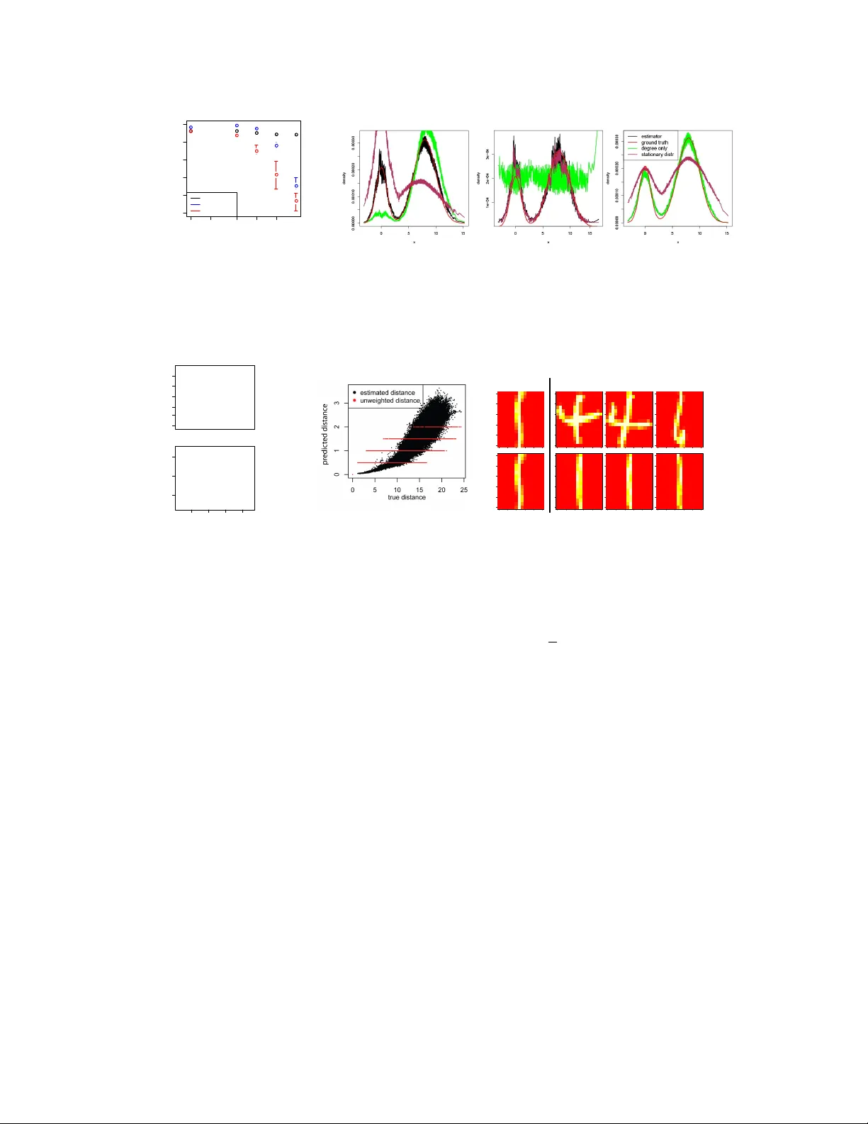
Metric r ecov ery fr om dir ected unweighted graphs T atsunori B. Hashimoto MIT CSAIL Cambridge, MA 02139 thashim@csail.mit.edu Y i Sun MIT Dept. Mathematics Cambridge, MA 02139 yisun@math.mit.edu T ommi S. Jaakk ola MIT CSAIL Cambridge, MA 02139 tommi@csail.mit.edu Abstract W e analyze directed, unweighted graphs obtained from x i ∈ R d by connecting verte x i to j if f | x i − x j | < ε ( x i ) . Examples of such graphs include k -nearest neighbor graphs, where ε ( x i ) varies from point to point, and, ar guably , many real world graphs such as co-purchasing graphs. W e ask whether we can recov er the underlying Euclidean metric ε ( x i ) and the associated density p ( x i ) giv en only the directed graph and d . W e show that consistent recovery is possible up to isometric scaling when the verte x degree is at least ω ( n 2 / (2+ d ) log( n ) d/ ( d +2) ) . Our estimator is based on a careful characterization of a random walk ov er the directed graph and the asso- ciated continuum limit. As an algorithm, it resembles the PageRank centrality metric. W e demonstrate empirically that the estimator performs well on simulated examples as well as on real-world co-purchasing graphs even with a small number of points and degree scaling as lo w as log ( n ) . 1 Introduction Data for unsupervised learning is increasingly av ailable in the form of graphs or networks. For example, we may analyze gene networks, social networks, or general co-occurrence graphs (e.g., built from purchasing patterns). While classical unsupervised tasks such as density estimation or clustering are naturally formulated for data in vector spaces, these tasks have analogous problems ov er graphs such as centrality and community detection. W e provide a step towards unifying unsu- pervised learning by recov ering the underlying density and metric directly from graphs. W e consider “unweighted directed geometric graphs” that are assumed to have been built from underlying (unobserv ed) points x i , i = 1 , . . . , n . In particular , we assume that graphs are formed by drawing an arc from each vertex i to its neighbors within distance ε n ( x i ) . Note that the graphs are typically not symmetric since the distance (the ε n -ball) may vary from point to point. By allowing ε n ( x i ) to be stochastic, e.g., depend on the set of points, the construction subsumes also typical k -nearest neighbor graphs. Arguably , graphs from top k friends/products, or co-association graphs may also be approximated in this manner . The key property of our f amily of geometric graphs is that their structure is completely characterized by two functions over the latent space: the local density p ( x ) and the local scale ε ( x ) . Indeed, global properties such as the distances between points can be recov ered by integrating these quantities. W e show that asymptotic behavior of random walks on the directed graphs relate to the density and metric. In particular , we show that random walks on such graphs with minimal degree at least 1 ω ( n 2 / (2+ d ) log( n ) d d +2 ) can be completely characterized in terms of p and ε using drift-diffusion processes. This enables us to recover both the density and distance giv en only the observed graph and the (hypothesized) underlying dimension d . The fact that we may recover the density (up to isometry) is surprising. For example, in k -nearest neighbor graphs, each vertex has degree exactly k . There is no immediate local information about the density , i.e., whether the corresponding point lies in a high-density region with small ball radii, or in a low-density region with large ball radii. The key insight of this paper is that random walks ov er such graphs naturally drift tow ard higher density regions, allo wing for density recovery . While the paper is primarily focused on the theoretical aspects of reco vering the metric and density , we believ e our results offer useful strategies for analyzing real-world networks. F or example, we analyzed the Amazon co-purchasing graph where an edge is dra wn from an item i to j if j is among the top k co-purchased items with i . These Amazon products may be co-purchased if they are similar enough to be complementary , but not so similar that they are redundant. W e extend our model to deal with connectivity rules shaped like an annulus, and demonstrate that our estimator can simultaneously recov er product similarities, product categories, and central products by metric embedding. 1.1 Relation to prior work The density estimation problem addressed by this paper was proposed and partially solved by von Luxbur g-Alamgir in [14] using integration of local density gradients ov er shortest paths. This es- timator has since been used for drawing graphs with ordinal constraints in [14] and graph down- sampling in [1]. Howe ver , the recovery algorithm is restricted to 1 -dimensional k -nearest neighbor graphs under the constraint k = ω ( n 2 / 3 log( n ) 1 3 ) . Our paper provides an estimator that works in all dimensions, applies to a more general class of graphs, and strongly outperforms that of von Luxbur g-Alamgir in practice. On a technical level, our work has similarities to the analysis of con ver gence of graph Laplacians and random walks on manifolds in [16, 6]. For example, in [13], Ting-Huang-Jordan used inﬁnitesimal generators to capture the con ver gence of a discrete Laplacian to its continuous equiv alent on k - nearest neighbor graphs. Howe ver , their analysis was restricted to the Laplacian and did not consider the latent recovery problem. In addition, our approach prov es con ver gence of the entire random walk trajectory and allows us to analyze the stationary distrib ution function directly . 2 Main results and pr oof outline 2.1 Problem setup Let X = { x 1 , x 2 , . . . } be an inﬁnite sequence of latent coordinate points drawn independently from a distribution with probability density p ( x ) in R d . Let ε n ( x i ) be a radius function which may depend on the draw of X . In this paper, we ﬁx a single draw of X and analyze the quenched setting. Let G n = ( X n , E n ) be the unweighted directed neighborhood graph with v ertex set X n = { x 1 , . . . , x n } and with a directed edge from i to j if and only if | x i − x j | < ε n ( x i ) . Fix now a large n . W e consider the random directed graph model given by observing the single graph G n . The model is completely speciﬁed by the latent function p ( x ) and the possibly stochastic ε n ( x ) . Under the conditions ( ? ) to be speciﬁed below , we solve the follo wing problem: Giv en only G n and d , form a consistent estimate of p ( x i ) and | x i − x j | up to proportionality constants. The conditions we impose on p ( x ) , ε n ( x ) , and the stationary density function π X n ( x ) of the sim- ple random walk X n ( t ) on G n are the following, which we refer to as ( ? ). W e assume ( ? ) holds throughout the paper . • The density p ( x ) is dif ferentiable with bounded ∇ log( p ( x )) on a path-connected compact domain D ⊂ R d with smooth boundary ∂ D . 2 • There is a deterministic continuous function ε ( x ) > 0 on D and scaling constants g n satisfying g n → 0 and g n n 1 d +2 log( n ) − 1 d +2 → ∞ so that, a.s. in the draw of X , g − 1 n ε n ( x ) con verges uniformly to ε ( x ) . • The rescaled density functions nπ X n ( x ) are a.s. uniformly equicontinuous. Remark. W e conjecture that the last condition in ( ? ) holds for any p and ε satisfying the other conditions in ( ? ) (see Conjecture S1.1). Let NB n ( x ) denote the set of out-neighbors of x so that y is in NB n ( x ) if there is a directed edge from x to y . The second condition in ( ? ) implies for all x ∈ X n that | NB n ( x ) | = ω ( n 2 d +2 log( n ) d d +2 ) . (1) 2.2 Statement of results Our approach is based on the simple random walk X n ( t ) on the graph G n . Let π X n ( x ) denote the stationary density of X n ( t ) . W e ﬁrst show that when appropriately renormalized, π X n ( x ) con verges to an explicit function of p ( x ) and ε ( x ) . Theorem 2.1. Given ( ? ), a.s. in X , we have nπ X n ( x ) → c p ( x ) ε ( x ) 2 , (2) for the normalization constant c − 1 = R p ( x ) 2 ε ( x ) − 2 dx . Combining this result with an estimate on the out-degree of points in G n giv es our general result on recov ery of density and scale. Let V d be the volume of the unit d -ball. Corollary 2.2. Assuming ( ? ), we have a.s. in X that n d − 2 d cV 2 /d d g 2 n ! d d +2 | NB n ( x ) | 2 d +2 π X n ( x ) d d +2 → p ( x ) and  1 c d/ 2 V d n 2 g d n  1 d +2 | NB n ( x ) | 1 d +2 π X n ( x ) − 1 d +2 → ε ( x ) . Pr oof. Immediate from the out-degree estimate p ( x ) ε n ( x ) d V d = | NB n ( x ) | /n and Theorem 2.1. Remark. If ε n ( x ) is constant, ev ery edge is bidirectional, so π X n ( x ) is proportional to the degree of x , and we recov er the standard ε -ball density estimator . Our estimator for density p ( x ) closely resembles the PageRank algorithm without damping [10]. In particular , for the k -nearest neighbor graph, it gives the same rank ordering as PageRank, and it reduces to PageRank as d → ∞ . When specializing to the k -nearest neighbor density estimation problem posed by von Luxbur g- Alamgir in [14], we obtain the following. Corollary 2.3. If ε n ( x ) is selected via the k -near est neighbors pr ocedur e with k = ω ( n 2 d +2 log( n ) d d +2 ) and satisﬁes the ﬁrst and last conditions in ( ? ), we have a.s in X that n cV 2 /d d ! d d +2 π X n ( x ) d d +2 → p ( x ) and  1 c d/ 2 V d n  1 d +2 π X n ( x ) − 1 d +2 → ε ( x ) . 3 Pr oof. By [4], the empirical ε n ( x ) induced by the k -nearest neighbors procedure satisﬁes the second condition of ( ? ) with ε ( x ) = 1 V 1 /d d p ( x ) 1 /d and g n = ( k /n ) 1 /d . 2.3 Outline of approach Our proof proceeds via the following steps. 1. As n → ∞ , the simple random walks X n ( t ) on G n con verge weakly to an It ˆ o process Y ( t ) , yielding weak con vergence between stationary measures. (Theorem 3.4) 2. The stationary density π Y ( x ) is explicitly determined via Fokk er-Planck equation. (Lemma 4.1) 3. Uniform equicontinuity of nπ X n ( x ) yields con vergence in density after rescaling. (Theo- rem 2.1) An intuitiv e explanation for our results is as follo ws. For large n , the simple random walk on G n , when considered with its original metric embedding, closely approximates the behavior of a drift- diffusion process. Both the process and the approximating walk mov e preferentially tow ard regions where p ( x ) is large and dif fuse more slowly out of regions where ε ( x ) is small. Occupation times therefore giv e us information about p ( x ) and ε ( x ) which allow us to recov er them. Formally , the con vergence of X n ( t ) to Y ( t ) follows by verifying the conditions of the Stroock- V aradhan criterion (Theorem 3.1) for con ver gence of discrete time Marko v processes to It ˆ o processes [12]. This criterion states that if the variance a n , expected value b n , a higher order moments ∆ n,α of a jump are continuous and well-controlled in the limit, then the process conv erges to an It ˆ o process under mild technical conditions. By using the Fokker -Planck equation, we can express the stationary density of this It ˆ o process solely in terms of p ( x ) and the out-degree | NB n ( x ) | . This allows us to estimate the density using only the unweighted graph. Let D and ∂ D be the closure and boundary of the support D of p ( x ) . Let B ( x, ε ) be the ball of radius ε centered at x . Let h n = g 2 n be the time rescaling necessary for X n ( t ) to have timescale equal to that of Y ( t ) . 3 Con vergence of the simple random walk to an It ˆ o process W e will verify the regularity conditions of the Stroock-V aradhan criterion (see [12, Section 6]). Theorem 3.1 (Stroock-V aradhan) . Let X n ( t ) be discr ete-time Markov processes deﬁned over a domain D with boundary ∂ D . Deﬁne the discrete time drift and dif fusion coefﬁcients by a ij n ( s, x ) = 1 h n X y ∈ NB n ( x ) 1 | NB n ( x ) | ( y i − x i )( y j − x j ) b i n ( s, x ) = 1 h n X y ∈ NB n ( x ) 1 | NB n ( x ) | ( y i − x i ) ∆ n,α ( s, x ) = 1 h n X y ∈ NB n ( x ) 1 | NB n ( x ) | | y − x | 2+ α . If we have a ij n ( s, x ) a.s − − → a ij ( s, x ) , b i n ( s, x ) a.s − − → b i ( s, x ) , ∆ n, 1 ( s, x ) a.s − − → 0 , and r egularity con- ditions to ensur e r eﬂection at ∂ D (Theorem S2.2 and Theorem S2.3), the time-r escaled stochastic pr ocesses X n ( b t/h n c ) con ver ge weakly in Skor okhod space D ([0 , ∞ ) , D ) to an It ˆ o pr ocess with r eﬂecting boundary condition d Y ( t ) = σ ( t, Y ( t )) dW t + b ( t, Y ( t )) dt, with W t a standar d d -dimensional Brownian motion and σ ( t, Y ( t )) σ ( t, Y ( t )) T = a ( t, Y ( t )) . Remark. The original result of Stroock-V aradhan was stated for D ([0 , T ] , D ) for all ﬁnite T ; our version for D ([0 , ∞ ) , D ) is equiv alent by [15, Theorem 2.8]. 4 The technical conditions of Theorem 3.1 enforcing reﬂecting boundary conditions are checked in Theorem S2.8 to Theorem S2.12. W e focus on con ver gence of the drift and diffusion coef ﬁcients. Lemma 3.2 (Strong LLN for local moments) . F or a function f ( x ) suc h that sup x ∈ B (0 ,ε ) | f ( x ) | < ε , given ( ? ) we have uniformly on x ∈ X n that 1 h n X y ∈ NB n ( x ) 1 | NB n ( x ) | f ( y − x ) a.s. − − → 1 h n Z y ∈ B ( x,ε n ( x )) f ( y − x ) p ( y ) p ε n ( x ) ( x ) dy . Pr oof. Denote the claimed v alue of the limit by µ ( x ) . For con ver gence in expectation, we condition on | NB n ( x ) | and apply iterated expectation to get E   1 h n X y ∈ NB n ( x ) 1 | NB n ( x ) | f ( y − x )   = E  1 h n E  f ( y − x )   | NB n ( x ) |   = µ ( x ) . For y ∈ B ( x, ε n ( x )) , we hav e | f ( y − x ) | ≤ ε n ( x ) , so Hoeffding’ s inequality yields P      1 h n X y ∈ NB n ( x ) 1 | NB n ( x ) | f ( y − x ) − µ ( x )     ≥ t  ≤ 2 exp  − 2 h 2 n | NB n ( x ) | 2 t 2 | NB n ( x ) | ε n ( x ) 2  = Θ  exp  − 2 g 2 n ε ( x ) − 2 | NB n ( x ) | t 2  (3) = o  n − 2 p ( x ) 2 /d t 2 ε ( x ) 4 ω (1)  = o ( n − 2 t 2 ω (1) ) for | NB n ( x ) | = ω  n 2 / ( d +2) log( n ) d/ ( d +2)  by (1). Borel-Cantelli then yields a.s. con ver gence. Remark. This limit holds ev en for stochastic ε n ( x ) as long as g − 1 n ε n ( x ) a.s. con verges uniformly to a deterministic continuous ε ( x ) . All statements up to (3) hold regardless of stochasticity of ε n ( x ) and the overall bound only requires conv ergence of ε n ( x ) . An example of such a graph is the k -nearest neighbors graph. W e now compute the drift and dif fusion coefﬁcients in terms of p ( x ) and ε ( x ) . Theorem 3.3 (Drift dif fusion coefﬁcients) . Almost sur ely on the draw of X , as n → ∞ , we have lim n →∞ a ij n ( s, x ) = δ ij 1 3 ε ( x ) 2 lim n →∞ b i n ( s, x ) = ∂ i p ( x ) 3 p ( x ) ε ( x ) 2 lim n →∞ ∆ n, 1 ( s, x ) = 0 , wher e δ ij is the Kr onecker delta function. Pr oof. By Lemma 3.2, a n , b n , and ∆ n, 1 con verge a.s. to their expectations, so it sufﬁces to verify that the integrals in Lemma 3.2 have the claimed limits. Because p is differentiable on D , for any x ∈ D we ha ve the T aylor expansion p ( x + y ) = p ( x ) + y · ∇ p ( x ) + o ( | y | 2 ) of p at x , where the con vergence is uniform on compact sets. For n large so that B ( x, ε n ( x )) lies completely inside D , substituting this expansion into the deﬁnitions of a n , b n , and ∆ n, 1 and integrating o ver spheres yields the result. Full details are in Theorem S2.14. 5 Theorem 3.4. Under ( ? ), as n → ∞ a.s. in the draw of X the pr ocess X n ( b t/h n c ) conver ges in D ([0 , ∞ ) , D ) to the isotr opic D -valued It ˆ o pr ocess Y ( t ) with r eﬂecting boundary condition deﬁned by d Y ( t ) = ∇ p ( Y ( t )) 3 p ( Y ( t )) ε ( Y ( t )) 2 dt + ε ( Y ( t )) √ 3 dW ( t ) . (4) Pr oof. Lemma 3.2 and Theorem 3.3 show that X n ( b t/h n c ) fulﬁlls the conditions of Theorem 3.1. The result follows from the Stroock-V aradhan criterion using the drift and diffusion terms from Theorem 3.3. 4 Con vergence and computation of the stationary distrib ution 4.1 Graphs satisfying condition ( ? ) The It ˆ o process Y ( t ) is an isotropic drift-diffusion process, so the Fokker -Planck equation [11] implies its density f ( t, x ) at time t satisﬁes ∂ t f ( t, x ) = X i  − ∂ x i [ b i ( t, x ) f ( t, x )] + 1 2 ∂ x 2 i [ a ii ( t, x ) f ( t, x )]  , (5) where b i ( t, x ) and a ii ( t, x ) are gi ven by b ( t, x ) = ∇ p ( x ) 3 p ( x ) ¯ ε ( x ) 2 and a ii ( t, x ) = 1 3 ¯ ε ( x ) 2 . Lemma 4.1. The pr ocess Y ( t ) deﬁned by (4) has absolutely continuous stationary measur e with density π Y ( x ) = cp ( x ) 2 ε ( x ) − 2 , wher e c was deﬁned in (2). Pr oof. By (5), to check that π Y ( x ) = cp ( x ) 2 ε ( x ) − 2 , it sufﬁces to sho w X i  ∂ x i p ( x )  p ( x ) − 1 ε ( x ) 2 c p ( x ) 2 ε ( x ) 2  − 1 2 ∂ x i  ε ( x ) 2 c p ( x ) 2 ε ( x ) 2   = 0 . W e now pro ve Theorem 2.1 by sho wing that a rescaling of π X n ( x ) con verges to π Y ( x ) . Pr oof of Theorem 2.1. The a.s. conv ergence of processes of Theorem 3.4 implies by Ethier-K urtz [5, Theorem 4.9.12] that the empirical stationary measures dµ n = n X i =1 π X n ( x i ) δ x i con verge weakly to the stationary measure dµ = π Y ( x ) dx for Y ( t ) . For any x ∈ X and δ > 0 , weak con vergence against 1 B ( x,δ ) yields X y ∈X n , | y − x | <δ π X n ( y ) → Z | y − x | <δ π Y ( y ) dy. By uniform equicontinuity of nπ X n ( x ) , for any ε > 0 there is small enough δ > 0 so that for all n we hav e       X y ∈X n , | y − x | <δ π X n ( y ) − |X n ∩ B ( x, δ ) | π X n ( x )       ≤ n − 1 |X n ∩ B ( x, δ ) | ε, 6 which implies that lim n →∞ π X n ( x ) p ( x ) n = lim δ → 0 lim n →∞ V − 1 d δ − d nπ X n ( x ) Z | y − x | <δ p ( y ) dy = lim δ → 0 lim n →∞ V − 1 d δ − d |X n ∩ B ( x, δ ) | π X n ( x ) = lim δ → 0 V − 1 d δ − d Z | y − x | <δ π Y ( y ) dy = π Y ( x ) . Combining with Lemma 4.1 yields the desired lim n →∞ nπ X n ( x ) = π Y ( x ) p ( x ) = c p ( x ) ε ( x ) 2 . 4.2 Extension to isotropic graphs T o obtain our stationary distribution in Theorem 2.1 we require only con ver gence to some It ˆ o process via the Stroock-V aradhan criterion. W e can achieve this under substantially more general conditions. W e deﬁne a class of neighborhood graphs on X n termed isotr opic ov er which we hav e consistent metric recov ery without knowledge of the graph construction method. Deﬁnition 1 (Isotropic) . A graph edge connection procedure on X n is isotropic if it satisﬁes: Distance kernel: The probability of placing a directed edge from i to j is deﬁned by a kernel function h ( r ij ) mapping locally scaled distances r ij = | x i − x j | ε n ( x i ) − 1 with ε n ( x ) obeying ( ? ) to probabilities Nonzero mass: The kernel function h ( r ) has nonzero integral R 1 0 h ( r ) r d − 1 dr > 0 . Bounded tails: For all r > 1 , h ( r ) = 0 . Continuity: The scaling nπ X n ( x ) of the stationary distribution is uniformly equicontinuous. This class of graph preserves the property that the random graph is entirely determined by the un- derlying density p ( x ) and local scale ε ( x ) ; this allows us to hav e the same tractable form for the stationary distribution. Both constant ε and k -nearest neighbor graphs are isotropic upon assumption of uniform equiconti- nuity . Another interesting class of graphs allowed by this generalization is truncated Gaussian ker- nels, where connecti vity probability decreases exponentially . Note that h ( r ) might not be monotonic or continuous in r ; one surprising example is h ( r ) = 1 [0 . 5 , 1] ( r ) , which deterministically connects points in an annulus. Corollary 4.2 (Generalization) . If a neighborhood graph is isotr opic, then the limiting stationary distribution follows Theor em 2.1, and the density and distances can be estimated by Cor ollary 2.2. Pr oof. W e check the Stroock-V aradhan condition stated in Theorem 3.1. For this, we use a ver- sion of Lemma 3.2 for isotropic graphs, which requires that the ball radius vanishes and that the neighborhood size scales as ω ( n 2 d +2 log( n ) d d +2 ) . V anishing neighborhood radius follows because bounded tails and the fact that the kernel is ev aluated on | x i − x j | ε n ( x i ) − 1 ensure the isotropic graph is a subgraph of the ε n ( x ) -ball graph. K olmogorov’ s strong law implies that the stochastic out-degree concentrates around its expectation. It has the correct scaling because the argument of h ( r ) is scaled by ε n ( x ) . See Theorem S3.2 for details. Thus the analogue of Lemma 3.2 holds. W e then check that the limiting local moments for isotropic graphs are proportional to those of ε n ( x ) -ball graphs in Lemma S3.3. All but one of the conditions for the Stroock-V aradhan criterion follow from this; the last Theorem S2.11 follo ws from the bounded ball structure of the connectivity kernel. 7 2.5 3.0 3.5 4.0 0.5 0.6 0.7 0.8 0.9 1.0 log_10 number of points correlation of metric vs graph density random walk, k=const random walk, k=log(n) random walk, k=sqrt(n) path integral, k=log(n) path integral, k=sqrt(n) Figure 1: Accuracy vs sample and neighborhood size. Path integral (green, maroon) is from Alamgir- von Luxbur g [14]. Our estimator (red, blue, black) is nearly perfect at all sample sizes and neighborhood sizes. Figure 2: Examples of four density estimates: our method (red) us- ing no metric information is indistinguishable from metric k -nearest neighbor (blue) and close to ground truth (black). Path integral esti- mator of Alamgir-von Luxbur g [14] (green) shows higher error in all cases. T o check that we obtain the same limiting process and stationary measure, note the ratios of integrals in Theorem 3.3 are unchanged in the isotropic setting. See Lemma S3.3 for details. Recovering the stationary distribution, density , and local scale is then done in the same manner as in the ε -ball setting. 5 Distance reco very via paths Our results in Theorem 2.1 giv e a consistent estimator for the density p ( x ) and the local scale ε ( x ) . These two quantities specify up to isometry the latent metric embedding of X . In order to reconstruct distances between non-neighbor points we weight the edges of G n by weights w ij = ε n ( x i ) and ﬁnd the shortest paths o ver this graph, which we call G n . The results of Alamgir- von Luxbur g [2, Section 4.1] show that in the k -nearest neighbor graph case, setting w ij = b ε n ( x i ) for the estimator b ε n of ε n results in consistent recov ery of pairwise distances. In Theorem S4.5, we giv e a straightforward extension of this approach to show that giv en any uni- formly con vergent estimator of ε n ( x ) , the shortest path on the weighted graph G n con verges to the geodesic distance. Applying standard metric multidimensional scaling then allows us to embed these distances and recov er the latent space up to isometry . 6 Empirical results W e demonstrate extremely good ﬁnite sample performance of our estimator in simulated density reconstruction problems and two real-world datasets. Some details such as exact graph degrees and distribution parameters are in the supplementary code which reproduces all ﬁgures in this paper . Standard graph statistics such as centrality and Jaccard index are calculated via the igraph package [3]. k -near est neighbor graphs W e compared our random-walk based estimator and the path-inte gral based estimator of von Luxbur g-Alamgir [14] to the metric k -nearest neighbor density estimator . The number of samples n was v aried from 100 to 20000 along with the sparsity lev el k (Figure 1). While our theoretical results suggest that both our algorithm and the path-integral estimator of von Luxburg-Alamgir [14] might fail to con verge at √ n and log ( n ) sparsity levels, in practice our estimator performs nearly perfectly at both low sparsity le vels. For constant degree k = 50 we achie ve near-perfect performance for all choices of n , while the path-integral estimator fails to con ver ge in the k = log ( n ) regime. Some speciﬁc examples of our density estimator with n = 2000 , k = 100 are shown in Figure 2. The examples are mixture of uniforms (left), mixture of Gaussians (center), and t -distribution (right). As predicted, our estimator tracks extremely closely with the metric k -nearest neighbor 8 1 2 5 10 20 0.5 0.6 0.7 0.8 0.9 1.0 dimensions correlation log(p), n=200 p, n=10000 p, n=200 Figure 3: Estimate performance degrades in high dimensions due to ov er-smoothing (blue and red), but the estimator is still highly accurate up to log concentration parameter (black). Figure 4: Example isotropic graphs. Our estimator (black) agrees with the true density (red) in all cases. Degree and stationary distribution (green and maroon) based density estimates work for some cases (right two panels) but cannot work if the degree is tied to spatial location (left). 6 5 4 7 3 6 3 1 0 1 7 0 1 1 7 7 4 8 0 1 4 8 7 4 8 7 3 7 4 1 3 6 7 4 1 3 7 7 4 5 4 2 7 4 1 3 7 7 4 0 6 3 2 0 8 6 6 2 0 8 7 8 2 0 9 0 2 2 0 8 1 2 0 8 3 3 2 8 2 2 0 8 1 4 4 8 9 8 9 6 7 6 1 9 7 0 8 0 4 6 8 0 0 3 0 8 0 9 0 3 8 0 1 2 2 9 0 6 6 5 9 2 0 9 1 4 1 2 7 1 0 9 0 8 0 7 9 1 3 0 4 4 3 5 1 6 8 5 4 4 6 8 4 4 8 6 4 0 2 3 9 8 6 8 9 3 5 6 8 0 2 2 6 8 4 1 0 2 7 1 0 2 2 7 1 0 9 2 7 0 4 8 0 8 7 2 7 1 3 2 7 3 2 2 2 7 1 0 2 2 8 5 4 2 2 7 8 7 0 2 7 1 0 2 6 0 2 7 6 0 8 2 7 1 1 0 1 7 7 6 4 4 6 2 9 1 1 9 0 3 1 1 8 1 0 3 1 6 1 1 7 5 5 3 6 5 0 6 8 8 0 0 0 1 4 9 5 7 0 0 0 1 6 0 1 9 8 6 0 1 9 8 6 8 0 0 9 6 8 5 4 4 9 4 0 8 6 4 8 1 2 1 2 1 2 6 8 0 2 1 3 0 2 3 2 3 5 8 0 2 7 9 0 0 0 0 6 8 9 7 7 9 4 9 1 2 9 4 5 3 8 5 7 1 8 0 1 4 6 5 5 3 2 0 1 0 6 6 6 6 0 9 0 2 6 0 5 5 9 6 1 7 7 7 6 1 8 2 0 6 0 5 2 1 6 1 8 6 6 6 0 9 0 2 6 0 2 5 6 0 9 0 2 6 0 5 2 1 6 0 5 4 6 6 4 7 3 6 1 8 2 1 6 0 9 0 2 6 0 4 3 5 6 0 5 6 1 8 2 0 6 0 9 0 2 6 1 8 0 1 6 0 5 2 2 6 1 7 6 1 6 0 4 7 3 1 8 2 6 0 9 0 2 6 1 7 0 1 6 0 5 2 2 0 9 2 7 6 0 9 0 2 6 1 8 2 1 6 1 9 1 3 6 0 9 0 2 6 1 9 0 0 4 6 2 6 1 8 0 1 4 6 9 9 2 9 7 1 0 2 8 0 7 0 2 9 7 1 0 2 8 2 3 4 2 8 2 1 2 2 8 6 5 8 2 8 7 3 9 2 8 2 1 7 2 8 2 7 2 0 0 9 2 2 8 3 6 2 8 3 0 3 2 8 6 0 1 2 8 1 0 2 8 2 6 5 2 8 2 6 2 8 4 3 2 8 2 3 2 8 1 1 2 3 2 2 6 2 1 2 2 2 1 1 6 2 7 0 2 2 4 0 1 2 3 4 5 2 3 0 6 0 9 3 0 0 3 0 0 8 8 3 0 0 8 3 3 0 2 4 0 3 0 8 1 5 3 0 2 7 4 3 0 8 0 9 3 0 0 3 0 2 3 0 2 4 7 8 1 1 1 1 2 1 3 7 2 1 0 3 8 0 3 7 1 3 0 8 5 1 6 8 5 7 0 8 9 1 1 9 8 0 0 0 5 2 0 0 1 1 2 0 0 3 7 5 9 4 0 2 9 7 4 1 0 2 1 3 0 0 2 2 1 5 0 2 1 0 9 0 2 1 4 6 0 1 7 2 0 0 1 9 0 6 0 2 1 3 8 0 1 9 7 0 0 1 8 4 1 0 1 3 6 4 0 2 6 0 1 0 1 8 3 0 9 1 0 4 9 8 0 7 2 0 0 6 5 0 9 0 0 6 3 0 0 0 9 0 7 0 0 9 3 4 4 0 6 9 0 0 7 0 8 0 6 6 0 0 9 1 8 6 5 4 0 0 6 0 4 0 0 7 5 8 0 0 2 3 0 0 6 6 0 0 9 0 7 0 0 9 2 3 0 0 9 1 2 0 0 6 9 7 0 7 5 4 2 3 5 5 7 1 8 8 6 0 0 1 8 0 2 0 2 0 4 8 2 8 0 6 0 2 1 3 2 9 7 1 0 4 0 1 8 5 0 2 3 8 5 3 4 5 8 9 1 0 7 3 8 1 5 2 4 6 2 0 6 0 1 0 7 4 6 9 1 2 2 3 2 0 4 8 8 3 8 6 6 6 1 4 9 7 0 0 6 9 7 4 0 5 9 8 0 0 2 9 0 9 8 4 0 8 4 9 5 5 0 4 8 2 3 2 2 6 9 8 4 8 0 8 4 0 7 2 0 8 5 0 0 6 5 3 7 0 6 9 2 5 7 6 5 7 1 9 6 5 4 6 8 5 4 4 6 8 0 0 9 6 8 8 0 3 6 8 1 1 4 8 5 0 2 7 8 5 7 1 8 8 5 2 2 7 1 1 8 9 3 1 9 0 1 1 9 9 7 7 1 9 7 1 4 1 9 1 1 9 7 1 4 1 9 7 2 6 0 0 0 6 6 2 2 2 4 6 3 1 6 4 6 3 1 4 6 6 5 4 7 3 9 0 0 1 9 0 0 4 5 7 0 0 6 2 7 0 8 0 9 7 0 0 9 4 0 2 9 6 4 0 5 0 5 4 1 0 1 7 2 4 0 7 9 4 1 2 2 8 4 2 5 4 1 4 1 7 0 1 4 1 5 3 1 4 0 9 1 4 4 3 0 1 4 2 1 0 1 4 3 1 1 4 1 4 7 2 4 1 9 4 2 5 0 1 4 2 5 0 1 4 2 5 0 1 4 1 1 3 9 1 4 7 0 3 2 1 2 3 2 1 2 0 2 2 1 2 6 8 2 1 2 0 2 1 2 6 2 1 4 0 4 2 1 7 0 1 1 2 1 2 2 8 3 0 3 6 6 3 0 3 2 6 3 0 3 5 6 0 3 4 9 3 0 3 0 2 6 3 0 3 4 4 3 0 3 2 7 1 9 9 6 6 1 9 8 0 3 1 9 7 1 3 1 9 5 1 9 0 6 1 9 8 0 4 1 9 7 1 3 6 7 2 1 7 7 7 4 8 6 7 0 6 2 7 2 4 1 7 2 5 0 3 7 2 5 1 2 7 2 2 0 3 7 2 0 3 2 3 7 4 0 5 3 8 1 5 1 3 8 1 3 4 3 7 0 7 5 3 8 1 3 8 3 8 1 1 7 3 7 2 0 2 9 6 0 7 3 7 0 8 3 8 0 5 0 1 9 8 9 9 1 9 9 6 8 1 9 7 2 0 1 9 8 8 0 4 0 3 1 9 7 1 1 1 9 7 1 1 1 7 7 1 7 4 0 4 1 7 6 0 1 1 7 0 1 3 1 7 5 7 3 1 7 0 1 1 1 7 5 7 3 1 7 3 6 0 1 7 8 3 7 1 7 5 4 7 1 7 0 6 6 1 7 6 0 4 3 0 0 1 7 7 6 3 7 5 7 3 1 6 9 1 5 7 3 4 0 1 1 7 0 5 5 1 7 3 1 1 7 5 7 3 1 7 3 0 6 1 7 0 2 1 7 2 6 8 1 7 4 0 7 1 7 3 3 3 1 7 0 1 1 1 7 0 5 5 1 9 7 2 0 1 9 7 2 6 0 0 1 1 9 8 0 4 1 9 7 0 3 1 9 7 1 1 9 8 5 0 1 9 7 0 7 9 7 0 0 1 9 8 0 3 9 8 5 1 9 8 9 1 0 1 9 6 1 9 0 6 7 0 2 2 7 7 1 1 0 0 1 9 7 2 6 0 0 1 0 1 9 8 0 5 1 9 8 9 7 9 8 9 9 1 4 2 0 1 8 0 2 1 7 1 1 0 1 9 7 2 6 0 0 1 0 0 5 4 0 1 0 5 3 4 5 0 5 4 0 1 0 5 4 0 1 0 5 6 4 1 0 8 8 7 0 2 8 8 2 0 3 7 7 0 0 6 2 2 6 0 6 0 3 8 0 6 7 9 0 0 8 7 0 6 0 9 1 3 5 0 6 1 0 3 0 6 0 8 7 0 6 0 8 7 0 4 0 9 6 0 4 9 6 3 4 9 2 0 0 4 7 5 1 5 3 6 3 1 4 0 1 4 1 0 6 0 4 9 0 4 9 3 0 1 4 2 0 0 9 7 2 0 1 9 7 2 0 9 9 7 1 0 2 9 7 2 1 0 1 8 6 4 2 1 9 3 2 0 1 9 3 3 5 1 8 0 4 9 1 8 1 0 1 1 5 9 1 8 9 0 1 1 8 7 0 4 1 9 1 0 1 1 9 1 3 2 1 9 1 0 1 1 9 1 0 1 1 9 2 5 5 1 9 1 0 4 1 9 1 2 4 1 9 1 4 1 1 9 0 1 3 1 9 0 0 3 1 9 1 3 0 1 9 1 0 1 1 9 0 3 1 1 0 1 1 0 3 1 9 0 1 0 1 0 7 1 9 0 1 5 1 9 0 1 6 5 4 7 3 6 3 1 0 1 7 0 1 1 7 7 4 8 0 1 4 8 7 4 8 7 3 7 4 1 3 6 7 4 1 3 7 7 4 5 4 2 7 4 1 3 7 7 4 0 6 3 2 0 8 6 6 2 0 8 7 8 2 0 9 0 2 2 0 8 1 2 0 8 3 3 2 8 2 2 0 8 1 4 4 8 9 8 9 6 7 6 1 9 7 0 8 0 4 6 8 0 0 3 0 8 0 9 0 3 8 0 1 2 2 9 0 6 6 5 9 2 0 9 1 4 1 2 7 1 0 9 0 8 0 7 9 1 3 0 4 4 3 5 1 6 8 5 4 4 6 8 4 4 8 6 4 0 2 3 9 8 6 8 9 3 5 6 8 0 2 2 6 8 4 1 0 2 7 1 0 2 2 7 1 0 9 2 7 0 4 8 0 8 7 2 7 1 3 2 7 3 2 2 2 7 1 0 2 2 8 5 4 2 2 7 8 7 0 2 7 1 0 2 6 0 2 7 6 0 8 2 7 1 1 0 1 7 7 6 4 4 6 2 9 1 1 9 0 3 1 1 8 1 0 3 1 6 1 1 7 5 5 3 6 5 0 6 8 8 0 0 0 1 4 9 5 7 0 0 0 1 6 0 1 9 8 6 0 1 9 8 6 8 0 0 9 6 8 5 4 4 9 4 0 8 6 4 8 1 2 1 2 1 2 6 8 0 2 1 3 0 2 3 2 3 5 8 0 2 7 9 0 0 0 0 6 8 9 7 7 9 4 9 1 2 9 4 5 3 8 5 7 1 8 0 1 4 6 5 5 3 2 0 1 0 6 6 6 6 0 9 0 2 6 0 5 5 9 6 1 7 7 7 6 1 8 2 0 6 0 5 2 1 6 1 8 6 6 6 0 9 0 2 6 0 2 5 6 0 9 0 2 6 0 5 2 1 6 0 5 4 6 6 4 7 3 6 1 8 2 1 6 0 9 0 2 6 0 4 3 5 6 0 5 6 1 8 2 0 6 0 9 0 2 6 1 8 0 1 6 0 5 2 2 6 1 7 6 1 6 0 4 7 3 1 8 2 6 0 9 0 2 6 1 7 0 1 6 0 5 2 2 0 9 2 7 6 0 9 0 2 6 1 8 2 1 6 1 9 1 3 6 0 9 0 2 6 1 9 0 0 4 6 2 6 1 8 0 1 4 6 9 9 2 9 7 1 0 2 8 0 7 0 2 9 7 1 0 2 8 2 3 4 2 8 2 1 2 2 8 6 5 8 2 8 7 3 9 2 8 2 1 7 2 8 2 7 2 0 0 9 2 2 8 3 6 2 8 3 0 3 2 8 6 0 1 2 8 1 0 2 8 2 6 5 2 8 2 6 2 8 4 3 2 8 2 3 2 8 1 1 2 3 2 2 6 2 1 2 2 2 1 1 6 2 7 0 2 2 4 0 1 2 3 4 5 2 3 0 6 0 9 3 0 0 3 0 0 8 8 3 0 0 8 3 3 0 2 4 0 3 0 8 1 5 3 0 2 7 4 3 0 8 0 9 3 0 0 3 0 2 3 0 2 4 7 8 1 1 1 1 2 1 3 7 2 1 0 3 8 0 3 7 1 3 0 8 5 1 6 8 5 7 0 8 9 1 1 9 8 0 0 0 5 2 0 0 1 1 2 0 0 3 7 5 9 4 0 2 9 7 4 1 0 2 1 3 0 0 2 2 1 5 0 2 1 0 9 0 2 1 4 6 0 1 7 2 0 0 1 9 0 6 0 2 1 3 8 0 1 9 7 0 0 1 8 4 1 0 1 3 6 4 0 2 6 0 1 0 1 8 3 0 9 1 0 4 9 8 0 7 2 0 0 6 5 0 9 0 0 6 3 0 0 0 9 0 7 0 0 9 3 4 4 0 6 9 0 0 7 0 8 0 6 6 0 0 9 1 8 6 5 4 0 0 6 0 4 0 0 7 5 8 0 0 2 3 0 0 6 6 0 0 9 0 7 0 0 9 2 3 0 0 9 1 2 0 0 6 9 7 0 7 5 4 2 3 5 5 7 1 8 8 6 0 0 1 8 0 2 0 2 0 4 8 2 8 0 6 0 2 1 3 2 9 7 1 0 4 0 1 8 5 0 2 3 8 5 3 4 5 8 9 1 0 7 3 8 1 5 2 4 6 2 0 6 0 1 0 7 4 6 9 1 2 2 3 2 0 4 8 8 3 8 6 6 6 1 4 9 7 0 0 6 9 7 4 0 5 9 8 0 0 2 9 0 9 8 4 0 8 4 9 5 5 0 4 8 2 3 2 2 6 9 8 4 8 0 8 4 0 7 2 0 8 5 0 0 6 5 3 7 0 6 9 2 5 7 6 5 7 1 9 6 5 4 6 8 5 4 4 6 8 0 0 9 6 8 8 0 3 6 8 1 1 4 8 5 0 2 7 8 5 7 1 8 8 5 2 2 7 1 1 8 9 3 1 9 0 1 1 9 9 7 7 1 9 7 1 4 1 9 1 1 9 7 1 4 1 9 7 2 6 0 0 0 6 6 2 2 2 4 6 3 1 6 4 6 3 1 4 6 6 5 4 7 3 9 0 0 1 9 0 0 4 5 7 0 0 6 2 7 0 8 0 9 7 0 0 9 4 0 2 9 6 4 0 5 0 5 4 1 0 1 7 2 4 0 7 9 4 1 2 2 8 4 2 5 4 1 4 1 7 0 1 4 1 5 3 1 4 0 9 1 4 4 3 0 1 4 2 1 0 1 4 3 1 1 4 1 4 7 2 4 1 9 4 2 5 0 1 4 2 5 0 1 4 2 5 0 1 4 1 1 3 9 1 4 7 0 3 2 1 2 3 2 1 2 0 2 2 1 2 6 8 2 1 2 0 2 1 2 6 2 1 4 0 4 2 1 7 0 1 1 2 1 2 2 8 3 0 3 6 6 3 0 3 2 6 3 0 3 5 6 0 3 4 9 3 0 3 0 2 6 3 0 3 4 4 3 0 3 2 7 1 9 9 6 6 1 9 8 0 3 1 9 7 1 3 1 9 5 1 9 0 6 1 9 8 0 4 1 9 7 1 3 6 7 2 1 7 7 7 4 8 6 7 0 6 2 7 2 4 1 7 2 5 0 3 7 2 5 1 2 7 2 2 0 3 7 2 0 3 2 3 7 4 0 5 3 8 1 5 1 3 8 1 3 4 3 7 0 7 5 3 8 1 3 8 3 8 1 1 7 3 7 2 0 2 9 6 0 7 3 7 0 8 3 8 0 5 0 1 9 8 9 9 1 9 9 6 8 1 9 7 2 0 1 9 8 8 0 4 0 3 1 9 7 1 1 1 9 7 1 1 1 7 7 1 7 4 0 4 1 7 6 0 1 1 7 0 1 3 1 7 5 7 3 1 7 0 1 1 1 7 5 7 3 1 7 3 6 0 1 7 8 3 7 1 7 5 4 7 1 7 0 6 6 1 7 6 0 4 3 0 0 1 7 7 6 3 7 5 7 3 1 6 9 1 5 7 3 4 0 1 1 7 0 5 5 1 7 3 1 1 7 5 7 3 1 7 3 0 6 1 7 0 2 1 7 2 6 8 1 7 4 0 7 1 7 3 3 3 1 7 0 1 1 1 7 0 5 5 1 9 7 2 0 1 9 7 2 6 0 0 1 1 9 8 0 4 1 9 7 0 3 1 9 7 1 1 9 8 5 0 1 9 7 0 7 9 7 0 0 1 9 8 0 3 9 8 5 1 9 8 9 1 0 1 9 6 1 9 0 6 7 0 2 2 7 7 1 1 0 0 1 9 7 2 6 0 0 1 0 1 9 8 0 5 1 9 8 9 7 9 8 9 9 1 4 2 0 1 8 0 2 1 7 1 1 0 1 9 7 2 6 0 0 1 0 0 5 4 0 1 0 5 3 4 5 0 5 4 0 1 0 5 4 0 1 0 5 6 4 1 0 8 8 7 0 2 8 8 2 0 3 7 7 0 0 6 2 2 6 0 6 0 3 8 0 6 7 9 0 0 8 7 0 6 0 9 1 3 5 0 6 1 0 3 0 6 0 8 7 0 6 0 8 7 0 4 0 9 6 0 4 9 6 3 4 9 2 0 0 4 7 5 1 5 3 6 3 1 4 0 1 4 1 0 6 0 4 9 0 4 9 3 0 1 4 2 0 0 9 7 2 0 1 9 7 2 0 9 9 7 1 0 2 9 7 2 1 0 1 8 6 4 2 1 9 3 2 0 1 9 3 3 5 1 8 0 4 9 1 8 1 0 1 1 5 9 1 8 9 0 1 1 8 7 0 4 1 9 1 0 1 1 9 1 3 2 1 9 1 0 1 1 9 1 0 1 1 9 2 5 5 1 9 1 0 4 1 9 1 2 4 1 9 1 4 1 1 9 0 1 3 1 9 0 0 3 1 9 1 3 0 1 9 1 0 1 1 9 0 3 1 1 0 1 1 0 3 1 9 0 1 0 1 0 7 1 9 0 1 5 1 9 0 1 Reconstructed Original (PCA) Figure 5: Reconstruction closely matches projection of the true metric. Figure 6: Distances estimated by our method are globally close to the true metric. Reference digit Digits ranked by similarity to reference Jaccard Estimated Figure 7: Items close in our weighted graph (bottom) are more similar than those under the Jaccard index (top). estimator (red and blue), as well as the true density (black). The path integral estimator has high estimate variance at points with lar ge density and fails to cope with the two mixture densities. V arying the dimension for an isotropic multiv ariate normal with k = √ n , we ﬁnd that a large number of points are required to maintain high accuracy as d grows large (red and blue lines in Figure 3). Howe ver , this is due to a global ‘ﬂattening’ of the density . Measuring the correlation between the true and estimated log probabilities show that up to a global concentration parameter , the estimator maintains high accuracy across a lar ge number of dimensions (black lines). Ker nel graphs W e validate the nonparametric estimator in Corollary 4.2 for kernel graphs by constructing three drastically different kernel graphs. In all cases, we sampled 5000 points with the connection probability following p i,j = exp( − ε ( x i ) − 1 | x i − x j | ) . W e varied the neighborhood structure ε in three ways: a constant kernel, ε ( x i ) ∝ 1 ; k -nearest neighbor k ernel: ε ( x ) ∝ 1 /ε k =100 ; and spatially varying k ernel ε ( x ) ∝ | x | . In Figure 4, we ﬁnd that our nonparametric estimator (black) always matches the ground truth (red). This example also shows that both the degree and the stationary distribution can be v alid density estimators under certain assumptions, but only our estimator can deal with arbitrary isotropic graph construction methods without assumptions. Metric reco very on real data As an example of metric reconstruction, we take the ﬁrst 2000 examples in the U.S. postal service (USPS) digits dataset [7] and construct an unweighted k -nearest neighbor graph. W e use our method to reconstruct the metric and perform similarity queries, and the Jaccard index was used to tie-break direct neighbors. The USPS digits dataset is known to hav e a high-density cluster of ones digits (orange). Results in Figure 5 show that we are able to successfully recover the density structure of the data (top). Inter- point distances estimated by our method (Figure 6, y -axis) show nearly linear agreement to the true metric ( x -axis) at short distances and high similarity globally . 9 0.5 0.6 0.7 0.8 0.9 1.0 300000 150000 50000 quantile cent r ality sales r ank r andom w alk betw eenness closeness Figure 8: Density estimates in the graph correlate well with sales rank, unlike other measures of centrality . 1 1 1 1 2 2 3 3 3 2 4 5 5 5 5 1 1 1 4 2 4 4 2 2 5 2 1 1 3 4 2 5 3 3 3 3 3 3 2 2 1 1 1 1 1 2 5 5 6 4 1 3 3 3 3 3 3 3 3 3 3 3 3 4 5 5 3 5 2 5 2 6 6 6 4 4 2 4 6 5 3 3 3 2 1 5 1 1 1 2 2 2 1 5 5 5 5 5 1 4 4 6 3 5 5 2 1 1 1 6 6 6 6 6 6 6 6 6 6 6 5 5 1 1 1 5 5 5 4 4 1 1 1 1 5 3 5 2 3 4 2 1 4 4 4 1 1 1 1 5 4 2 5 1 1 1 1 4 1 5 5 1 1 1 1 1 1 5 1 1 1 1 6 4 4 4 4 5 4 5 3 1 1 1 3 1 5 4 6 1 1 1 3 3 3 5 5 4 1 1 1 1 1 4 3 3 3 3 3 5 5 4 2 2 2 4 5 6 5 2 2 3 2 3 2 5 1 1 6 6 3 3 1 1 6 6 6 6 3 3 3 3 3 1 1 1 1 5 1 4 3 6 5 5 4 3 3 4 4 5 5 5 4 4 4 5 5 5 5 5 3 3 3 2 5 3 3 2 3 1 1 5 5 4 4 2 4 1 5 5 5 5 5 5 5 2 1 5 1 1 1 1 2 2 2 5 1 1 1 5 1 1 1 4 1 1 1 1 1 4 4 1 5 4 3 5 1 5 4 4 4 5 1 1 1 1 2 1 1 4 3 3 3 3 4 4 2 1 1 1 1 2 5 5 4 5 2 4 4 2 2 2 2 2 3 3 3 3 3 3 5 6 5 2 5 3 3 3 3 4 1 1 1 1 4 4 4 1 1 1 1 1 4 2 1 1 1 1 4 3 3 4 4 4 6 1 3 5 5 5 5 5 5 4 4 4 2 4 2 5 1 1 5 2 2 2 5 3 3 1 2 4 4 4 4 4 1 5 4 4 6 6 2 3 3 5 6 6 4 6 6 6 6 6 6 1 1 5 5 1 1 1 2 1 1 1 3 4 5 3 1 5 5 4 5 2 2 2 2 5 5 5 1 4 4 4 5 4 1 5 5 5 5 5 2 2 2 2 2 6 6 1 1 1 1 1 1 1 6 6 6 6 6 1 1 1 1 2 2 6 4 4 4 5 1 1 2 1 1 1 5 5 5 5 2 3 3 3 3 3 3 1 4 4 4 3 1 5 1 3 3 4 4 2 1 2 2 3 3 1 4 4 5 5 3 2 3 4 6 6 3 4 4 2 1 4 4 4 4 4 5 5 5 1 1 6 6 1 4 5 5 4 4 5 4 1 1 5 5 5 5 1 2 1 1 1 1 1 2 1 6 6 6 6 6 6 6 1 1 1 1 1 1 1 3 2 2 5 5 2 3 3 3 1 1 3 5 4 4 6 5 2 4 5 1 5 2 4 2 1 6 6 6 6 4 5 3 2 2 2 4 4 4 4 5 5 1 1 2 2 5 3 3 3 1 5 2 1 2 2 5 1 1 1 1 1 1 1 1 4 3 3 3 3 6 6 6 4 2 4 4 4 5 4 6 6 6 6 6 6 1 5 2 5 3 2 2 4 4 2 2 3 3 3 2 1 3 4 4 3 3 4 4 4 4 1 6 6 6 1 1 6 4 6 4 1 3 1 6 2 2 4 5 5 5 5 3 3 3 3 3 3 2 5 5 3 3 5 1 5 2 3 3 3 5 5 5 1 1 1 1 6 6 6 6 6 6 6 6 6 6 1 1 1 4 4 1 5 3 3 3 1 2 2 5 5 5 5 5 1 1 1 5 4 5 1 2 2 2 1 2 2 2 2 1 6 6 6 6 6 6 6 6 6 4 4 4 3 5 5 2 1 1 5 3 4 4 1 4 4 3 3 3 2 3 1 3 3 1 2 1 1 1 1 1 1 3 3 2 2 3 4 4 4 4 5 4 5 2 1 1 5 1 1 1 1 1 5 4 3 5 1 1 3 3 3 3 2 1 1 5 1 1 1 5 5 3 5 4 1 1 3 3 5 6 5 2 6 1 1 1 1 1 1 6 5 5 3 1 2 3 3 2 2 2 3 3 1 1 1 1 1 1 3 3 4 3 3 3 3 3 4 4 4 1 6 6 2 2 6 6 5 5 5 2 1 1 6 2 2 2 2 5 4 4 4 4 3 3 3 3 2 2 2 1 1 5 4 6 3 3 3 4 3 3 3 3 3 3 3 1 1 1 1 1 5 5 3 3 3 3 3 5 5 5 6 3 4 4 2 3 1 2 2 2 2 5 6 6 5 2 2 2 2 5 5 5 2 5 4 4 4 1 3 3 1 1 3 3 3 1 1 1 1 4 5 1 1 4 2 2 4 4 2 6 3 3 2 5 1 1 1 5 3 5 5 5 2 2 1 3 5 4 5 1 1 1 1 2 2 1 1 5 3 3 3 1 3 3 3 3 3 4 5 5 5 1 3 2 2 1 1 3 1 2 6 6 5 5 2 3 3 3 1 5 5 3 3 3 5 4 3 3 1 2 2 5 1 1 6 1 1 1 1 1 5 5 5 5 5 5 2 1 1 3 2 4 5 2 4 4 2 1 1 5 2 2 2 1 1 1 1 1 1 1 1 1 1 1 1 2 2 3 3 3 4 4 4 2 2 3 3 3 3 1 1 4 1 3 3 4 4 5 6 6 2 3 3 1 1 5 3 5 2 2 5 4 4 5 5 5 4 4 4 3 3 3 5 3 2 3 5 1 1 1 1 1 3 6 4 3 3 3 3 3 5 5 5 3 3 3 3 3 2 1 1 3 5 1 3 5 2 3 3 1 4 5 5 5 1 1 1 1 1 2 2 3 3 3 4 5 1 1 1 1 4 2 2 5 4 2 5 5 2 5 5 4 1 1 1 1 1 2 2 4 5 3 3 3 3 5 5 3 1 4 1 1 1 1 1 2 4 4 5 2 1 3 3 6 4 1 1 1 5 3 3 3 1 5 5 3 3 3 2 2 2 5 1 1 2 5 5 5 5 2 1 5 1 1 1 5 2 3 3 5 5 5 5 5 5 6 5 5 3 3 4 6 4 4 3 3 3 1 1 1 1 1 5 1 1 3 2 4 4 1 1 1 3 3 6 6 6 1 3 3 2 6 6 2 1 2 2 2 1 3 5 5 1 5 2 3 3 5 4 2 2 1 4 3 2 2 1 1 1 1 5 5 5 5 5 4 1 1 4 4 4 4 3 3 5 3 3 3 3 1 4 1 1 1 6 6 4 2 1 1 4 1 2 4 6 1 3 3 3 1 1 1 1 1 1 1 3 3 3 1 5 1 1 1 1 1 1 1 1 1 6 1 2 2 2 3 3 3 3 5 3 3 3 5 5 6 4 5 6 6 6 6 6 3 1 1 4 5 5 1 1 1 3 3 2 2 6 6 6 1 3 1 1 1 1 1 1 1 2 1 2 2 4 4 5 4 5 1 1 2 1 1 2 2 5 4 5 5 3 4 1 6 2 1 3 1 2 2 2 2 1 4 3 2 2 1 1 1 1 5 1 2 1 4 2 2 2 2 1 3 3 2 1 1 5 1 5 1 5 1 2 3 1 1 4 5 4 4 3 3 3 2 2 2 1 1 5 5 1 2 2 1 1 1 5 5 3 2 5 5 3 4 3 6 3 3 4 1 2 2 2 5 3 1 4 4 4 4 3 3 3 1 1 5 2 3 5 1 4 5 5 3 3 3 5 5 1 1 1 2 1 1 5 5 5 3 3 3 5 5 2 4 3 5 4 1 5 5 2 3 3 3 4 4 3 3 1 1 5 2 2 2 2 4 5 5 3 3 3 3 1 1 3 3 5 1 1 1 5 3 5 5 5 5 1 1 1 5 5 2 4 6 1 3 3 3 3 3 3 1 5 5 3 2 3 3 3 4 5 4 4 4 4 3 3 6 4 4 4 4 4 5 1 6 6 2 2 2 2 3 3 3 1 1 2 5 5 6 3 3 3 5 5 6 6 4 5 5 2 2 3 4 4 5 5 5 1 5 5 5 5 2 5 2 5 4 1 1 2 5 1 1 1 1 1 1 1 1 5 5 1 1 1 3 1 1 1 2 2 1 5 5 5 2 2 2 2 2 3 6 1 5 4 3 3 5 1 1 1 3 3 5 1 1 1 2 6 6 6 6 5 5 5 6 6 6 5 5 1 1 5 4 5 5 4 1 1 3 1 1 1 5 5 3 4 5 5 1 5 3 3 2 2 5 1 3 5 5 3 6 3 4 4 4 4 4 4 3 3 1 2 2 3 3 4 5 3 3 5 4 3 5 1 2 4 1 1 1 1 3 3 1 1 5 2 1 2 1 3 3 3 3 3 3 2 1 3 3 6 3 2 1 1 5 2 2 2 5 3 2 1 3 3 1 1 4 1 6 4 3 3 3 2 1 5 5 5 3 3 3 5 3 1 3 1 3 1 5 5 2 2 1 1 3 3 3 3 4 2 3 1 1 2 5 5 1 2 4 2 5 1 1 4 4 5 1 4 5 4 3 4 1 1 1 1 1 6 1 1 1 1 1 1 1 5 1 1 4 4 5 2 5 5 4 4 1 1 5 5 5 5 2 2 5 3 1 1 5 4 3 5 3 3 1 1 1 1 1 5 2 4 1 4 2 1 5 6 6 5 6 6 1 5 1 2 6 6 6 6 6 3 4 2 5 1 1 3 4 6 6 6 6 1 1 1 2 3 1 1 1 1 5 1 5 2 3 3 5 4 1 3 3 6 5 5 3 1 3 2 4 4 4 1 1 1 1 1 3 6 6 6 1 1 2 2 5 1 1 1 3 1 4 1 2 1 1 3 3 6 3 3 5 3 3 3 3 3 1 1 2 1 3 1 1 1 3 2 2 1 3 1 1 3 3 6 6 1 1 5 5 3 3 3 6 4 2 1 1 2 3 1 1 1 1 1 1 1 2 3 4 3 3 2 2 1 5 5 5 3 2 2 3 2 1 6 6 6 6 2 2 4 1 1 1 1 1 3 3 1 1 3 1 3 1 3 3 2 6 5 3 3 5 1 2 3 3 2 5 2 2 6 3 1 2 4 2 2 2 3 6 6 1 1 3 3 3 3 2 5 3 3 5 5 1 5 4 4 2 1 6 6 3 1 5 5 6 3 3 1 3 6 3 1 5 1 4 5 5 3 6 3 5 1 4 3 4 4 3 3 2 4 2 5 4 1 2 1 6 1 1 5 6 6 6 3 2 1 6 1 1 4 5 1 3 5 4 5 2 1 3 3 1 1 2 3 1 4 4 1 3 3 3 1 2 1 1 1 1 3 3 3 3 5 6 6 1 4 6 6 6 2 3 5 5 1 1 4 1 1 1 5 1 3 2 3 3 3 3 1 5 1 6 1 2 1 3 6 6 1 1 1 5 6 2 5 1 1 1 1 1 4 2 1 1 3 5 2 2 2 2 2 5 5 6 6 1 4 5 3 5 5 5 3 1 2 2 3 4 5 3 1 1 5 1 4 4 4 1 2 1 4 5 1 6 6 5 3 4 3 3 4 3 5 1 1 5 3 3 5 1 6 1 5 5 5 5 4 6 4 5 6 3 3 1 2 6 4 6 3 5 2 −10 −5 0 5 10 15 20 25 −5 0 5 10 15 PC1 PC2 1 2 3 4 5 6 Religion & Spirituality[22] History[9] Computers & Internet[5] Literature & Fiction[17] Nonfiction[53] Classical[85] Figure 9: Embeddings from estimated distances recover the separation be- tween different product cate gories. Performing a similarity query on the data (Figure 7) shows that the our reconstructed distances (bottom row) have a more coherent set of similar digits when compared to the Jaccard index (top row) [8]. The behavior of the unweighted Jaccard similarity is due to a kno wn problem with shortest paths in k -nearest neighbor graphs preferring lo w density regions [14]. Classics Literature Classical music Philosophy The Prince The Stranger Beethoven: Symphonien Nos. 5 & The Practice of Everyday Life The Communist Manifesto The Myth of Sisyphus Mozart: Symphonies Nos. 35-41 The Society of the Spectacle The Republic The Metamorphosis Mozart: V iolin Concertos The Production of Space W ealth of Nations Heart of Darkness Tchaikovsk y: Concerto No. 1/Rac Illuminations On W ar The Fall Beethoven: Symphonies Nos. 3 & Space and Place: The Perspectiv T able 1: T op 4 clusters formed by mapping each item to its mode (ﬁrst row). Each group is a coherent genre. Amazon co-purchasing data Finally , we recover density and metric on a real network dataset with no ground truth. W e analyzed the largest connected component of the Amazon co-purchasing network dataset [9]. Each vertex is a product on amazon.com along with its category and sales rank, and each directed edge represents a co-purchasing recommendation of the form “person who bought x also bought y . ” This dataset naturally fulﬁlls our assumptions of having edges that are asymmetric, where edges represent a notion of similarity in some space. The items that lie in regions of highest density should be archetypal products for a category , and therefore be more popular . W e show that the density estimates using our method with d = 10 show a strong positi ve association between density and sales (Figure 8). W e found that this effect persisted regardless of choice of d . Other popular measures of network centrality such as betweenness and closeness fail to display this ef fect. W e then attempted metric recov ery using our random walk based reconstruction (Figure 9). F or visualization purposes, we used multidimensional scaling on the recovered metric to embed points belonging to categories with at least two hundred items. The embedding shows that our method captures the separation across different product categories. Notably , nonﬁction and history have substantial overlap as expected, while classical music CD’ s and computer science books hav e little ov erlap with the other clusters. Analyzing the modes of the density estimate by clustering each point to its local mode, we ﬁnd coherent clusters where top items serve as archetypes for the cluster (T able 1). This suggests that there may be a close connection between clustering in a metric space and community detection in network data. The o verall performance of our method on density estimation and metric recovery for the Amazon dataset suggests that when a metric assumption is appropriate, our random walk based metric quantities can be used directly for centrality and cluster estimates on a network. 7 Conclusions W e have presented a simple e xplicit identity linking the stationary distribution of a random walk on a neighborhood graph to the density and neighborhood size. The density estimator constructed by in verting this identity shows an extremely rapid con ver gence to the metric k -nearest neighbor density estimator across a range of data point count, sparsity le vel, and distribution type (Figures 1,2). W e also generalized the theorem to a large class of graph construction 10 techniques and demonstrated that the choice of construction technique matters little for accuracy (Figures 4). Our estimator performed well on real-world data, recovering underlying metric information in test data (Figures 6,7) and predicting popular Amazon products through density estimates (Figure 8). There are se veral open questions left unanswered by our work. Our results required that the graphs be of degree k = ω ( n 2 / ( d +2) log( n ) d/ ( d +2) ) rather than the log ( n ) required for connectivity . Our simulation results seem to suggest than even near the log( n ) regime our estimator performs nearly perfectly , suggesting that the true degree lo wer bound may be much lower . The close connection of our density estimate to PageRank suggests that combining the latent spatial map with vector space estimates may lead to highly effecti ve and theoretically principled network algorithms. References [1] M. Alamgir , G. Lugosi, and U. v on Luxb urg. Density-preserving quantization with application to graph downsampling. In COLT , 2014. [2] M. Alamgir and U. V . Luxbur g. Shortest path distance in random k-nearest neighbor graphs. In Pr oceedings of the 29th International Conference on Machine Learning (ICML-12) , pages 1031–1038, 2012. [3] G. Csardi and T . Nepusz. The igraph software package for complex network research. Inter- Journal , Comple x Systems:1695, 2006. [4] L. P . Devroye and T . W agner . The strong uniform consistency of nearest neighbor density estimates. The Annals of Statistics , pages 536–540, 1977. [5] S. N. Ethier and T . G. Kurtz. Markov pr ocesses: characterization and con ver gence . John W iley & Sons, 1986. [6] M. Hein, J.-y . Audibert, U. V . Luxburg, and S. Dasgupta. Graph Laplacians and their con ver - gence on random neighborhood graphs. Journal of Machine Learning Researc h , page 2007, 2006. [7] J. J. Hull. A database for handwritten text recognition research. P attern Analysis and Mac hine Intelligence, IEEE T ransactions on , 16(5):550–554, 1994. [8] P . Jaccard. ´ Etude comparati ve de la distribution ﬂorale dans une portion des Alpes et des Jura. Bulletin del la Soci ´ et ´ e V audoise des Sciences Naturelles , 37:547–579, 1901. [9] J. Leskov ec, L. A. Adamic, and B. A. Huberman. The dynamics of viral marketing. ACM T ransactions on the W eb (TWEB) , 1(1):5, 2007. [10] L. Page, S. Brin, R. Motwani, and T . W inograd. The PageRank citation ranking: Bringing order to the web . 1999. [11] H. Risken. F okker-Planc k Equation . Springer , 1984. [12] D. Stroock and S. V aradhan. Diffusion processes with boundary conditions. Communications on Pur e and Applied Mathematics , 24:147–225, 1971. [13] D. Ting, L. Huang, and M. I. Jordan. An analysis of the con vergence of graph Laplacians. In Pr oceedings of the 27th International Conference on Machine Learning (ICML-10) , pages 1079–1086, 2010. [14] U. V on Luxburg and M. Alamgir . Density estimation from unweighted k -nearest neighbor graphs: a roadmap. In Advances in Neural Information Pr ocessing Systems , pages 225–233. Springer , 2013. [15] W . Whitt. Some useful functions for functional limit theorems. Math. Oper . Res. , 5(1):67–85, 1980. [16] W . W oess. Random walks on inﬁnite graphs and groups - a survey on selected topics. Bull. London Math. Soc , 26:160, 1994. 11 Supplemen tary pro ofs for: Metric recov ery from directed un weigh ted graphs Octob er 26, 2014 Con ten ts 1 Conjecture on uniform equicontin uit y of the rescaled stationary distribution 1 2 F ull pro of of Theorem 2.1 2 2.1 Deﬁnition of the ob jects . . . . . . . . . . . . . . . . . . . . . . . 3 2.2 Quantities used in the Stroo c k-V aradhan criterion . . . . . . . . 4 2.3 Statement of the Stro ock-V aradhan criterion . . . . . . . . . . . 5 2.4 V eriﬁcation of the Stro ock-V aradhan conditions . . . . . . . . . . 7 2.4.1 Momen t conditions . . . . . . . . . . . . . . . . . . . . . . 7 2.4.2 Boundary conditions . . . . . . . . . . . . . . . . . . . . . 8 2.5 Completing the pro of of Theorem S2.1 . . . . . . . . . . . . . . . 10 3 Generalizing to isotropic graphs 12 4 Recov ery of distances via ball-radii 15 4.1 Outline of pro of approach . . . . . . . . . . . . . . . . . . . . . . 15 4.2 The case of exact knowledge of ε n . . . . . . . . . . . . . . . . . . 15 4.3 The case of stochastic estimates of ε n . . . . . . . . . . . . . . . 17 1 Conjecture on uniform equicon tin uit y of the rescaled stationary distribution In the conditions ( ? ) we imposed, we required the uniform equicontin uit y of nπ X n . Without this condition, our pro of tec hnique implies the w eak conv ergence X x ∈X n π X n ( x ) δ x → π Y ( x ) dx of the empirical stationary measures of X n ( t ) to the stationary measure of Y ( t ). The additional imp osition of uniform equicon tin uity was required solely to up- grade this con vergence to a con vergence of the rescaled discrete densit y functions 1 to the contin uous density function. W e conjecture that this contin uity is true in general. Conjecture S1.1. Given the other c ontinuity and sc aling c onditions on p ( x ) and ε n ( x ) in ( ? ) , nπ X n ( x ) is a.s. uniformly e quic ontinuous. W e discuss a few reasons wh y we might b eliev e this conjecture to hold. • In the case of constant ε n ( x ), nπ X n ( x ) is prop ortional to | NB n ( x ) | , hence con verges to p ( x ) uniformly . The conjecture therefore holds in this case. • Our empirical results pro duce robust results across a broad range of n , ε ( x ), and p ( x ). One p ossible explanation would b e that Conjecture S1.1 holds for all datasets constructed according to ( ? ). • F or x, y ∈ X n , let r n ( x ) denote the exp ected ﬁrst return time to x and c n ( x, y ) denote the exp ected comm ute time from x to y . It is known that π X n ( x ) = 1 r n ( x ) , so to show that nπ X n ( x ) is uniformly equicontin uous, it suﬃces to show that n r n ( x ) is uniformly equicontin uous. Notice that r n ( x ) ≤ c n ( x, y ) + r n ( y ) + c n ( y , x ) and that r n ( y ) ≤ c n ( x, y ) + r n ( x ) + c n ( y , x ) , whic h together imply that | r n ( x ) − r n ( y ) | ≤ | c n ( x, y ) + c n ( y , x ) | . This relates contin uity of r n ( x ) and hence π X n ( x ) to the commute time c n ( x, y ). On the other hand, our techniques using the Stro ock-V aradhan criterion yield con vergence of the simple random walk X n ( t ) to the Itˆ o pro cess Y ( t ) in D ([0 , ∞ ) , D ) without assumption of uniform equicontin u- it y . In a scaling limit, this should lead to a relation b et ween c n ( x, y ) and a rescaling of the commute time of the corresp onding Itˆ o pro cess. In future w ork, w e in tend to use this result to relate a scaling of c n ( x, y ) to | x − y | and approac h Conjecture S1.1 in conjunction with new metho ds for metric estimation. 2 F ull pro of of Theorem 2.1 The goal of this section will be to give a fully rigorous pro of of Theorem 3.4 from the main text. W e ﬁrst restate the theorem as Theorem S2.1. 2 Theorem S2.1. Under ( ? ), if h n → g 2 n as n → ∞ , then a.s. in X , the pr o c ess X n ( b t/h n c ) c onver ges in D ([0 , ∞ ) , D ) to the isotr opic D -value d Itˆ o pr o c ess Y ( t ) with r eﬂe cting b oundary c ondition deﬁne d by d Y ( t ) = ∇ p ( Y ( t )) 3 p ( Y ( t )) ε ( Y ( t )) 2 dt + ε ( Y ( t )) √ 3 dW ( t ) , (1) wher e the pr e cise me aning of the r eﬂe cting b oundary c ondition is given in Sub- se ction 2.1. Our technique is an application of the Stro ock-V aradhan criterion (see [2, Theorem 6.3]) for conv ergence of discrete time Mark o v pro cesses in a b ounded domain to drift-diﬀusion pro cesses with reﬂecting b oundary conditions in that domain. In what follo ws, we preserve the notation used by Stro ock-V aradhan in [2] whenever p ossible. 2.1 Deﬁnition of the ob jects In this subsection, we recall in detail the problem setup. W e are given an inﬁnite sequence X = { x 1 , x 2 , . . . } of latent co ordinate p oin ts drawn indep enden tly from a distribution with probability densit y p ( x ) in R d supp orted on a compact domain D ⊂ R d with smo oth b oundary ∂ D . W e ma y then ﬁnd a b ounded C 2 function φ ( x ) on R d so that D = { x | φ ( x ) > 0 } , ∂ D = { x | φ ( x ) = 0 } , and |∇ φ ( x ) | ≥ 1 on ∂ D . W e ﬁx a single random dra w of X and analyze the quenched setting. W e are then giv en a radius function ε n ( x i ) which may dep end on the draw of X and a scaling factor g n so that lim n →∞ g − 1 n ε n ( x ) = ε ( x ) for some deterministic ε ( x ) on D . Let G n = ( X n , E n ) b e the unw eighted directed neigh b orhoo d graph with v ertex set X n = { x 1 , . . . , x n } and with a directed edge from i to j if and only if | x i − x j | < ε n ( x i ) . Note that G n is sto c hastic and dep ends on the sp eciﬁc realization of X n whic h is drawn. Let X n ( t ) b e the simple random walk on the directed graph G n so that X n ( t ) is a discrete-time Marko v pro cess with state space X n . W e normalize the timestep of X n ( t ) to b e h n = g 2 n and identify X n ( t ) with the contin uous time pro cess giv en by t 7→ X n ( b t/h n c ). F rom now on, w e refer to these tw o pro cesses in terchangeably . In Theorem S2.1, we wish to show that X n ( t ) con verges w eakly in D ([0 , ∞ ) , D ) to the con tinuous-time con tinuous-space Itˆ o process Y ( t ) deﬁned by (1) with re- ﬂecting b oundary conditions. W e in terpret the b oundary conditions in terms of 3 the submartingale condition of [2]. That is, we deﬁne the v ector function γ ( s, x ) to b e the normal vector to ∂ D at x whose length is normalized so that h γ ( s, x ) , ∇ φ ( x ) i = 1 . T ake also the scalar function ρ ( s, x ) = 0. T ogether, γ and ρ sp ecify the b oundary conditions in the following sense. W e say that a pro cess Y ( t ) solves the submartingale problem for a , b , ρ , and γ if for an y function f ∈ C 1 , 2 0 ([0 , ∞ ) × D ) satisfying ρ ( ∂ f /∂ t ) + h γ , ∇ f i ≥ 0 on [0 , ∞ ) × ∂ D , the random v ariable f ( t, Y ( t )) − Z t 0 ( f s + L s f )( s, Y ( s )) 1 D ( Y ( s )) ds is a submartingale, where L s f = 1 2 d X i,j =1 a ij ∂ 2 f ∂ x i ∂ x j + d X j =1 b j ∂ f ∂ x j . As explained in [2], when ρ = 0, this formulation is equiv alent to specifying that Y ( t ) satisﬁes (1) on the interior of D and has reﬂecting b oundary conditions on ∂ D . 2.2 Quan tities used in the Stro o c k-V aradhan criterion W e now deﬁne the moment and b oundary quantities whic h are used in the Stro ock-V aradhan criterion. W e follow the notations of [2]. Our discrete time Mark ov pro cess X n ( t ) has time increment h n = g 2 n and transition kernel Π n ( x, A ) = p ( X n ( t + 1) ∈ A | X n ( t ) = x ) = |X n ∩ A ∩ B ( x, ε n ( x )) | |X n ∩ B ( x, ε n ( x )) | for x ∈ X n , where we recall that X n ∩ B ( x, ε n ( x )) = NB n ( x ). The moment quan tities in [2] are the discrete time drift b n , diﬀusion a n , and tail ∆ n,α co eﬃcien ts, deﬁned for x ∈ X n b y a ij n ( s, x ) = 1 h n Z ( y i − x i )( y j − x j )Π n ( x, dy ) = 1 h n X y ∈ NB n ( x ) ( y i − x i )( y j − x j ) | NB n ( x ) | b i n ( s, x ) = 1 h n Z ( y i − x i )Π n ( x, dy ) = 1 h n X y ∈ NB n ( x ) y i − x i | NB n ( x ) | ∆ n,α ( s, x ) = 1 h n Z | y − x | 2+ α Π n ( x, dy ) = 1 h n X y ∈ NB n ( x ) | y − x | 2+ α | NB n ( x ) | . 4 The b oundary conditions are sp eciﬁed b y γ and ρ , where we recall that ρ ≡ 0. W e note that γ has the alternate expression γ ( s, x ) = C γ ( x ) lim n →∞ ε n ( x ) − 1 Z | y | <ε n ( x ) y p ( x + y ) p ε n ( x ) ( x ) dy , where p r ( x ) = R | y | 0. These theorems will dep end on several conditions whic h w e lab el A-E and F1-4 and chec k in the next subsection. Remark. By [3, Theorem 2.8], conv ergence in D ([0 , T ] , D ) for all T > 0 implies con vergence D ([0 , ∞ ) , D ). F urther, b y [1, Theorem 4.9.12], this implies w eak con vergence of the stationary measures of X n ( t ) to the stationary measure of Y ( t ). The ﬁrst theorem yields tightness of measures of X n ( t ) on Skorokhod space. Theorem S2.2 ([2, Theorem 6.1]) . Supp ose a discr ete time Markov pr o c ess X n ( t ) satisﬁes the fol lowing c onditions. A. (b ounde d tail mass): F or some α > 0 , as n → ∞ , we have sup 0 ≤ t ≤ T sup x ∈ G ∆ n,α ( t, x ) → 0 . B. (al l lar ge drifts ar e r eﬂe ctions): Ther e exists M and c such that for al l n > n 0 , | b n ( t, x ) | > M implies h∇ φ ( x ) ,b n ( t,x ) i | b n ( t,x ) | ≥ c . C. (b ounde d drift outside b oundary): F or every δ > 0 ther e exists some M δ < ∞ such that for al l n > n 0 , | b n ( t, x ) | > M δ implies φ ( x ) < δ . D. (b ounde d diﬀusion): Ther e exists M < ∞ such that for al l n > n 0 , sup 0 ≤ t ≤ T sup x ∈ G || a n ( t, x ) || ≤ M , wher e || · || denotes the F r ob enius norm. 5 Then, the family of distributions P n x induc e d by X x n ( t ) over tr aje ctories is c on- ditional ly c omp act in D ([0 , T ] , D ) . Mor e over, any we ak limit of these is c onc en- tr ate d on the subset C ([0 , T ] , D ) ⊂ D ([0 , T ] , D ) . The next theorem yields conv ergence of X n ( t ) under conv ergence of the momen t quan tities and some regularity conditions on the b oundary . Theorem S2.3 ([2, Theorem 6.3]) . Supp ose X n ( t ) satisﬁes the fol lowing. E. (c onver genc e of c o eﬃcients): Drift and diﬀusion c o eﬃcients a n and b n c onver ge uniformly on c omp act subsets K ⊂ [0 , T ] × D to some a and b . F1. (r eﬂe ctivity at absorbing b oundary): Given ( t, y ) ∈ J 1 and ε > 0 , ther e exists n 0 < ∞ , δ 0 > 0 such that if | t − s | < δ 0 , | x − y | < δ 0 , n > n 0 and h∇ φ ( x ) , a n ( s, x ) ∇ φ ( x ) i < δ 0 the fol lowing hold: | a n ( s, x ) | < ε and | b n ( s, x ) − ρ − 1 ( t, y ) γ ( t, y ) | < ε. F2. (b ounde d drift under absorption): Given ( t, y ) ∈ J 1 ther e exist M 0 < ∞ and δ 0 > 0 such that if | s − t | < δ 0 and | y − x | < δ 0 , then | b n ( s, x ) | ≤ M 0 for al l n. F3. (drift dominates diﬀusion on r eﬂe ction): Given ( t, y ) ∈ J 0 and M < ∞ ther e exist δ 0 > 0 and n 0 < ∞ such that if | t − s | < δ 0 , | x − y | < δ 0 , n > n 0 , and h∇ φ ( x ) , a n ( s, x ) ∇ φ ( x ) i < δ 0 , we have | b n ( s, x ) | ≥ M . F4. (drifts at b oundary simulate r eﬂe ction): Given ( t, y ) ∈ J 0 and ε > 0 ther e exist δ 0 > 0 , n < ∞ and M < ∞ such that if | s − t | < δ 0 , | x − y | < δ 0 , n > n 0 , and | b n ( s, x ) | > M , then     b n ( s, x ) h b n ( s, x ) , ∇ φ ( x ) i − γ ( t, y )     < ε. Then any we ak limit Y ( t ) of X n ( t ) in D ([0 , T ] , D ) solves the submartingale pr oblem for a , b , ρ , and γ . Finally , we state a criterion for uniqueness of solution to the submartingale problem for a , b , ρ , and γ . Theorem S2.4 ([2, Theorem 5.8]) . Supp ose a , b , ρ , and γ ar e time indep endent and satisfy the fol lowing c onditions. 1. a is c ontinuous, symmetric, and p ositive deﬁnite on D ; 2. b is b ounde d and me asur able; 6 3. γ is b ounde d, lo c al ly Lipschitz, and on ∂ D satisﬁes h γ ( x ) , ∇ φ ( x ) i ≥ β > 0; 4. ρ ( x ) is b ounde d, c ontinuous, and non-ne gative. Then the solution to the submartingale pr oblem for a , b , ρ , and γ is unique. Com bining Theorem S2.2, Theorem S2.3, and Theorem S2.4 yields the fol- lo wing conclusion. Corollary S2.5. Supp ose that X n ( t ) satisﬁes the c onditions of The or em S2.2, The or em S2.3, and The or em S2.4. Then X n ( t ) c onver ges to Y ( t ) in D ([0 , T ] , D ) . Pr o of. By Theorem S2.2, some subsequential limit of X n ( t ) exists. Theo- rem S2.3 implies that an y suc h limit is a solution to the submartingale problem for a , b , ρ , and γ , so the uniqueness of Theorem S2.4 yields the desired result. 2.4 V eriﬁcation of the Stro o c k-V aradhan conditions W e now v erify each of the nine conditions necessary for w eak conv ergence. Con- ditions F1 and F2 are v acuous b ecause J 1 is empt y for us. W e now verify each of the remaining conditions. 2.4.1 Momen t conditions Theorem S2.6 (Condition A) . As n → 0 , we have sup 0 ≤ t ≤ T sup x ∈ D ∆ n, 1 ( t, x ) → 0 . Sp e ciﬁc al ly, we have ∆ n, 1 ( s, x ) → lim n →∞ 1 h n Z | y | <ε n ( x ) | y | 3 p ( x + y ) p ε n ( x ) ( x ) dy = 0 . Pr o of. F rom Lemma 3.2 with f ( x ) = | x | 3 . Theorem S2.7 (Condition E) . The se quenc es of drift and diﬀusion c o eﬃcients a n → a and b n → b c onver ge uniformly on c omp act subsets K ⊂ [0 , T ] × G . Mor e sp e ciﬁc al ly, the limiting quantities ar e a ij n ( s, x ) → lim n →∞ 1 h n Z | y | <ε n ( x ) y i y j p ( x + y ) p ε n ( x ) ( x ) dy b i n ( s, x ) → lim n →∞ 1 h n Z | y | <ε n ( x ) y i p ( x + y ) p ε n ( x ) ( x ) dy . Pr o of. F rom Lemma 3.2 with f ( x ) = x and f ij ( x ) = x i x j . 7 2.4.2 Boundary conditions Theorem S2.8 (Condition C) . F or δ > 0 , ther e exists M δ < ∞ and n 0 so that for n > n 0 , | b n ( t, x ) | > M δ implies φ ( x ) < δ . Pr o of. On the compact set { φ ( x ) ≥ δ } , b n ( t, x ) con verges uniformly by Theo- rem S2.7 and Theorem S2.14 to 1 3 ∇ p ( x ) p ( x ) ε ( x ) 2 , hence is uniformly b ounded on this set. Theorem S2.9 (Condition D) . The diﬀusion term a n is uniformly b ounde d by some M < ∞ so that sup s,x,n || a n ( s, x ) || ≤ M . Pr o of. By deﬁnition the diﬀusion term a ij n ( s, x ) = 1 h n X y ∈ NB n ( x ) 1 | NB n ( x ) | ( y i − x i )( y j − x j ) is an av erage of num b ers b ounded by ε n ( x ) 2 h n . This quantit y conv erges to the b ounded function ε ( x ) as n → ∞ , yielding the result. Theorem S2.10 (Condition F3) . Given ( t, y ) ∈ J 0 and M < ∞ , ther e ex- ist δ 0 > 0 and n 0 < ∞ so that if | t − s | < δ 0 , | x − y | < δ 0 , n > n 0 , and h∇ φ ( x ) , a n ( s, x ) ∇ φ ( x ) i < δ 0 , then | b n ( s, x ) | ≥ M . Pr o of. F or any δ 1 > 0, by Lemma 3.2, we may choose n 0 large enough s o that for all n > n 0 and x ∈ X n , we hav e || a n ( s, x ) − a ( s, x ) || < δ 1 , whic h implies that h∇ φ ( x ) , a n ( s, x ) ∇ φ ( x ) i ≥  1 3 ε ( x ) 2 − δ 2 1 )  |∇ φ ( x ) | 2 . Because ε ( y ) > 0, we can c ho ose δ 0 > 0 so that ε ( x ) 2 is uniformly b ounded a wa y from 0 on | x − y | < δ 0 , hence c ho osing δ 1 small mak es the condition v acuous. Theorem S2.11 (Condition F4) . Given ( t, y ) ∈ J 0 and ε > 0 , ther e exist δ 0 > 0 , n 0 < ∞ , and M < ∞ so that if | t − s | < δ 0 , | x − y | < δ 0 , n > n 0 , and | b n ( s, x ) | > M , then     b n ( s, x ) h b n ( s, x ) , ∇ φ ( x ) i − γ ( t, y )     < ε. Pr o of. F or an y ε > 0, ﬁx M > 0 to b e chosen later. Cho ose δ 0 small enough so that if | x − y | < 2 δ 0 , we hav e     p ( x ) − p ( y ) − ( y − x ) · ∇ p ( y ) p ( y )     < C 1 8 for some uniform C 1 . By Lemma 3.2 and the fact that |∇ φ ( x ) | ≥ 1 on ∂ D and is contin uous, we ma y choose n 0 large enough so that for all n > n 0 and | x − y | < δ 0 , we hav e • ε n ( x ) < δ 0 ; • | ε n ( x ) 2 h − 1 n − ε ( x ) 2 | < C 2 for a uniform C 2 > 0; •    b n ( s, x ) − E [ b n ( s, x )]    < M / 2 for x ∈ X n ; •    b n ( s,x ) h b n ( s,x ) , ∇ φ ( x ) i − E [ b n ( s,x )] h E [ b n ( s,x )] , ∇ φ ( x ) i    < ε/ 2 for x ∈ X n . If | b n ( s, x ) | > M for n > n 0 , then    E [ b n ( s, x )]    > M / 2 . No w, orien t the coordinate axes so that the ﬁrst co ordinate axis lies on the normal vector from x to ∂ D , and let τ b e the distance from x to ∂ D . In this case, we compute E [ b 1 n ( s, x )] = h − 1 n Z z ∈ B ( x,ε n ( x )) ∩ D ( z 1 − x 1 ) p ( z ) p ε n ( x ) ( x ) dy = ε n ( x ) − min { τ , ε n ( x ) } h n + 1 6 ∂ 1 p ( x ) p ( x ) ε n ( x ) 2 + τ 2 h n + C 3 and for i > 1 that E [ b i n ( s, x )] = 1 6 ∂ i p ( x ) p ( x ) ε n ( x ) 2 h n + C 4 (2) for error terms C 3 and C 4 indep enden t of n . Cho osing M large enough, we ﬁnd τ < (1 − C 5 ( M )) ε n ( x ) for a constant C 5 ( M ) > 0 indep endent of n , which implies that E [ b 1 n ( s, x )] ≥ C 5 ( M ) ε n ( x ) h n + 1 6 ∂ 1 p ( x ) p ( x ) ε n ( x ) 2 + τ 2 h n + C 3 . (3) No w, notice that γ ( s, y ) is a vector purely in the normal direction to ∂ D at y normalized so that h γ ( s, y ) , ∇ φ ( y ) i = 1. Because the constants C 3 , C 4 , C 5 ( M ) in (3) and (2) are indep enden t of n , all terms in these equations aside from C 5 ( M ) ε n ( x ) h n scale to constants as we take n 0 and M large, so E [ b n ( s,x )] h E [ b n ( s,x )] , ∇ φ ( x ) i b ecomes arbitrarily close to a vector purely in the normal direction to ∂ D from x . Cho osing δ 0 small enough makes these v ectors coincide up to error ε/ 2, whic h giv es the result when com bined with the b ound     b n ( s, x ) h b n ( s, x ) , ∇ φ ( x ) i − E [ b n ( s, x )] h E [ b n ( s, x )] , ∇ φ ( x ) i     < ε/ 2 w e obtained by taking n 0 large. 9 Theorem S2.12 (Condition B) . Ther e exist M , c , and n 0 so that for al l n > n 0 , | b n ( t, x ) | > M implies h∇ φ ( x ) , b n ( t, x ) i | b n ( t, x ) | ≥ c. Pr o of. By deﬁnition, γ ( t, x ) is uniformly bounded ab o ve by some C 0 . Now, by compactness of ∂ D = J 0 , there exists some δ > 0 so that each x ∈ { φ ( y ) < δ } has a corresp onding x 0 ∈ δ D so that the conclusion of Theorem S2.11 applies with ε = C 0 / 2. T aking M = M δ and n 0 from Theorem S2.8 for this δ and applying Theorem S2.11 yields that h∇ φ ( x ) , b n ( t, x ) i | b n ( t, x ) | ≥ 2 C 0 . 2.5 Completing the pro of of Theorem S2.1 By C orollary S2.5, to complete the proof of Theorem S2.1, it suﬃces for us to compute the limiting terms a and b and to verify the conditions of Theo- rem S2.4 for uniqueness of the submartingale problem. W e b egin b y computing the limiting a and b , for which we will need the following lemma. Lemma S2.13. F or d ≥ 2 , let B d ( r ) b e the d -dimensional b al l of r adius r and V d ( r ) = V d r d b e its volume. As r → 0 , we have Z B d ( r ) x n i dx = ( 0 n o dd 2 V d − 1 n +1 r n + d + o ( r n + d ) n even and Z B d ( r ) x n i x m j dx = 0 if n o dd . Pr o of. If n is odd, b oth claims follo w b ecause the integrands are o dd functions in tegrated ov er symmetric domains. If n is even, for the ﬁrst claim we compute Z B d ( r ) x n i dx = Z r − r V d − 1 ( p r 2 − x 2 ) x n dx = 2 V d − 1 n + 1 r n + d + o ( r n + d ) . Theorem S2.14 (Drift diﬀusion co eﬃcien ts) . The limiting inte gr als for drift and diﬀusion ar e a ii n ( s, x ) = 1 h n  1 3 ε n ( x ) 2 + o ( ε n ( x ) 2 )  → 1 3 ε ( x ) 2 a ij n ( s, x ) = 1 h n o ( ε n ( x ) d +2 ) 2 V d − 1 p ( x ) ε n ( x ) d + o ( ε n ( x ) d ) → 0 b i n ( s, x ) = 1 h n  1 3 ∂ i p ( x ) p ( x ) ε n ( x ) 2 + o ( ε n ( x ) 2 )  → ∂ i p ( x ) 3 p ( x ) ε ( x ) 2 ∆ n, 1 ( x, s ) = 1 h n  ε n ( x ) d +4 p ( x ) V d − 1 + o ( ε n ( x ) d +4 ) 2 V d − 1 p ( x ) ε n ( x ) d + o ( ε n ( x ) d )  → 0 . 10 Pr o of. Because p is diﬀerentiable on D , for any x ∈ D we ha v e the T a ylor expansion p ( x + y ) = p ( x ) + y · ∇ p ( x ) + o ( | y | 2 ) of p at x , where the con vergence is unif orm on compact sets. F or n large enough so that the ball of radius ε n ( x ) centered at x lies completely inside D , we can substitute this expansion in to the deﬁnitions of a n and b n . Using Lemma S2.13 to estimate the resulting expressions yields a ii n ( s, x ) = 1 h n R | y | <ε n ( x ) y 2 i p ( x ) + y 2 i y · ∇ p ( x ) + y 2 i o ( | y | 2 ) dy R | y | <ε n ( x ) p ( x ) + y · ∇ p ( x ) + o ( | y | 2 ) dy = 1 h n 2 3 V d − 1 p ( x ) ε n ( x ) d +2 + o ( ε n ( x ) d +2 ) 2 V d − 1 p ( x ) ε n ( x ) d + o ( ε n ( x ) d ) = 1 h n  1 3 ε n ( x ) 2 + o ( ε n ( x ) 2 )  and a ij n ( s, x ) = 1 h n R | y | <ε n ( x ) y i y j p ( x ) + y i y j y · ∇ p ( x ) + y i y j o ( | y | 2 ) dy R | y | <ε n ( x ) p ( x ) + y · ∇ p ( x ) + o ( | y | 2 ) dy = 1 h n o ( ε n ( x ) d +2 ) 2 V d − 1 p ( x ) ε n ( x ) d + o ( ε n ( x ) d ) and b i n ( s, x ) = 1 h n R | y | <ε n ( x ) y i p ( x ) + y i y · ∇ p ( x ) + y i o ( | y | 2 ) dy R | y | <ε n ( x ) p ( x ) + y · ∇ p ( x ) + o ( | y | 2 ) dy = 1 h n 2 3 V d − 1 ∂ i p ( x ) p ( x ) ε n ( x ) d +2 + o ( ε n ( x ) d +2 ) 2 V d − 1 p ( x ) ε n ( x ) d + o ( ε n ( x ) d ) = 1 h n  1 3 ∂ i p ( x ) p ( x ) ε n ( x ) 2 + o ( ε n ( x ) 2 )  . Deﬁning S d ( r ) to b e the surface area of a radius r ball in d dimensions, w e ﬁnd ∆ n, 1 ( s, x ) = 1 h n R | y | <ε n ( x ) | y | 3 p ( x ) + | y | 3 p ( x ) + | y | 3 o ( | y | 3 ) dy R | y | <ε n ( x ) p ( x ) + y · ∇ p ( x ) + o ( | y | 2 ) dy = 1 h n R ε n ( x ) 0 r 3 S d ( r ) p ( x ) + o ( ε n ( x ) d +4 ) 2 V d − 1 p ( x ) ε n ( x ) d + o ( ε n ( x ) d ) = 1 h n o ( ε n ( x ) d +4 ) 2 V d − 1 p ( x ) ε n ( x ) d + o ( ε n ( x ) d ) . The result follo ws b y taking the n → ∞ limit in each estimate and recalling that h n w as chosen so that h − 1 n ε n ( x ) 2 → ¯ ε n ( x ) 2 and h − 1 n ε n ( x ) 2+ α → 0. The ﬁnal con vergence is uniform on compact sets b ecause the conv ergence of the initial T aylor expansion w as, each in tegration estimate preserves uniformit y , and the limit h − 1 n ε n ( x ) 2 → ¯ ε ( x ) 2 is uniform ov er all of D . 11 Pr o of of The or em S2.1. T o pro ve Theorem S2.1, it remains only to chec k the conditions of Theorem S2.4. Condition (1) follo ws b ecause a ( x ) = 1 3 ε ( x ) 2 · I is a contin uous m ultiple of the identit y . Condition (2) follows b ecause b ( x ) = 1 3 ∇ p ( x ) p ( x ) ε ( x ) 2 is evidently b ounded and measurable. F or Condition (3), γ is eviden tly b ounded, lo cally Lipschitz b ecause it is a normalized vector normal to the smo oth ∂ D , and h γ ( x ) , ∇ φ ( x ) i = 1 by deﬁnition. Finally , Condition (4) is evident b ecause ρ ≡ 0. 3 Generalizing to isotropic graphs In this section, w e giv e details on how to generalize our results for ε n ( x )-ball graphs to isotropic graphs. The approach is exactly parallel; we verify the conditions of the Stro ock-V aradhan criterion and consider the limiting rescaled stationary distribution. W e give in this section the necessary estimates of the minimal degree and the drift and diﬀusion terms. W e ﬁrst presen t a technical lemma. Lemma S3.1. F or d ≥ 2 , L et S d ( r ) b e the d -dimensional shel l of r adius r and V d ( r ) = C d r d b e its volume. As r → 0 , we have Z S d ( r ) x n i dx = ( 0 n o dd 2 C d − 1 n +1 ( n + d ) r n + d − 1 + o ( r n + d − 1 ) n even and Z S d ( r ) x n i x m j dx = 0 if n o dd . Pr o of. This follows by diﬀerentiating Lemma S2.13. Let us no w consider an isotropic graph mo del with kernel function h ( r ). In particular, this implies that there is an edge from x i to x j with probabilit y h ( | x i − x j | ε n ( x i ) − 1 ) and that Z 1 0 h ( r ) r d − 1 dr > 0 . W e c haracterize the minimal out-degree in this setting. Theorem S3.2 (Minimal out-degree) . F or an isotr opic gr aph with kernel h ( r ) satisfying ( ? ), we have the almost sur e c onver genc e ε n ( x ) − d | NB n ( x ) | |X n ∩ B ( x, ε n ( x )) | → C ( h ) p ( x ) for a c onstant C ( h ) indep endent of x and n , which implies that the minimal de gr e e | NB n ( x ) | = ω ( n 2 / ( d +2) log( n ) d/ ( d +2) ) . 12 Pr o of. The out-degree of a vertex is the indep endent sum of binary v ariables, eac h with probability h ( | x i − x j | ε n ( x i ) − 1 ), so Kolmolgorov’s strong la w yields ε n ( x ) − d | NB n ( x ) | |X n ∩ B ( x, ε n ( x )) | → E  ε n ( x ) − d | NB n ( x ) | |X n ∩ B ( x, ε n ( x )) |  . Let y ( r , θ ) b e the radial representation of y and let C = 2 C d +1 ( n + d ) n +1 b e the constan ts in Lemma S3.1. The desired exp ected v alue is the integral E  ε n ( x ) − d | NB n ( x ) | |X n ∩ B ( x, ε n ( x )) |  = Z y ∈ B ( x,ε n ( x )) p ( x + y ) h ( | y | ε − 1 n ( x )) dy ∼ ε n ( x ) − d Z y ∈ B ( x,ε n ( x )) ( p ( x ) + ∇ p ( x ) · y ) h ( | y | ε − 1 n ( x )) dy = ε n ( x ) − d Z ε n ( x ) 0 Z θ ∈ S d ( r ) ( p ( x ) + ∇ p ( x ) · y ( r , θ )) h ( r ) dy dθ = C p ( x ) ε n ( x ) − d Z ε n ( x ) 0 h ( r ) r d − 1 dr + ε n ( x ) − d Z ε n ( x ) 0 h ( r ) r d − 1 Z θ ∈ S d (1) ∇ p ( x ) · y (1 , θ ) drdθ . The latter term is zero by Lemma S3.1 since it is the in tegral of the odd function y (1 , θ ) ov er a symmetric domain. Now take the substitution s = r /ε n ( x ) to obtain E  ε n ( x ) − d | NB n ( x ) | |X n ∩ B ( x, ε n ( x )) |  = C p ( x ) Z 1 0 h ( s ) s d − 1 ds. The Kolmogorov strong law provides concen tration around this v alue. Noting that ε n ( x ) d = ω ( n 2 / ( d +2) log( n ) d/ ( d +2) ) gives the asymptotic claim. Since Theorem S3.2 guarantees that asymptotically w e achiev e the necessary minimal num b er of p oints, and h ( x ) is zero for x > 1, Lemma 3.2 applies to sho w the moment conditions in the Stro o c k-V aradhan criterion. F or the b oundary conditions, note that C, D, and F3 only require conv ergence of coeﬃcients in Lemma S3.3 to those in Theorem S2.14. Conditions F4 and B rely on tw o facts, the uniform conv ergence of co eﬃcien ts giv en by Lemma S3.3, and the asymmetry induced by the b oundary (3), the pro of of which is parallel to the one given for ε -ball graphs. Therefore, to complete the pro of the generalization, it remains only to compute the limiting drift and diﬀusion co eﬃcien ts. Lemma S3.3 (Polynomial integrals with resp ect to kernel) . Under the same c onditions as The or em S3.2, for any p ositive inte ger α we have Z y ∈ B ( x,ε n ( x )) y α i p ( x + y ) h ( | y | ε − 1 n ( x )) dy ∼ V ( h, α ) Z y ∈ B ( x,ε n ( x )) y α i p ( x + y ) dy as n → ∞ for a c onstant V ( h, α ) indep endent of n with V ( h, 1) = V ( h, 2) . 13 Pr o of. P erform the same T aylor approximation and radial decomposition as in Theorem S3.2 to obtain Z y ∈ B ( x,ε n ( x )) y α i p ( x + y ) h ( | y | ε − 1 n ( x )) dy ∼ Z ε n ( x ) 0 Z θ ∈ S d ( r ) y i ( r , θ ) α ( p ( x ) + ∇ p ( x ) · y ( r , θ )) h ( r ε − 1 n ( x )) dr dθ. F or α an o dd integer, by Lemma S3.1 w e hav e Z y ∈ B ( x,ε n ( x )) y α i p ( x + y ) h ( | y | ε − 1 n ( x )) dy ∼ Z ε n ( x ) 0 h ( r ε − 1 n ( x )) r α + d Z θ ∈ S d (1) y i (1 , θ ) α ∇ p ( x ) · y (1 , θ ) drdθ = ∂ p i ( x ) Z 1 0 h ( r ) r α + d dr ε n ( x ) α + d Z θ ∈ S d (1) y i (1 , θ ) α +1 dθ ∼ V ( h, α ) Z y ∈ B ( x,ε n ( x )) y α i p ( x + y ) dy for V ( h, α ) = ( α + d + 1) Z 1 0 h ( r ) r α + d dr . If α is an ev en in teger, we hav e Z y ∈ B ( x,ε n ( x )) y α i p ( x + y ) h ( | y | ε − 1 n ( x )) dy ∼ Z ε n ( x ) 0 h ( r ε − 1 n ( x )) r α + d − 1 Z θ ∈ S d (1) y i (1 , θ ) α p ( x ) dr dθ = p ( x ) Z ε n ( x ) 0 h ( r ε − 1 n ( x )) r α + d − 1 dr Z θ ∈ S d (1) y i (1 , θ ) α dθ = p ( x ) ε n ( x ) α + d Z 1 0 h ( r ) r α + d − 1 dr Z θ ∈ S d (1) y i (1 , θ ) α dθ ∼ V ( h, α ) Z y ∈ B ( x,ε n ( x )) y α i p ( x + y ) dy for V ( h, α ) = ( α + d ) Z 1 0 h ( r ) r α + d − 1 dr . The limits of drift and diﬀusion terms in Theorem S2.14 dep end only on ra- tios of these in tegrals for α = 1 , 2, so applying Lemma S3.3 sho ws that the limits for isotropic graphs are identical to the ones for ε -ball graphs. The remainder of the analysis pro ceeds unchanged. 14 4 Reco v ery of distances via ball-radii W e will prov e that given the ball radii ε n ( x i ), we can reco ver point-to-point dis- tances if x i are lo cated in a conv ex domain. Otherwise, w e reco v er the geo desic distances. Our goal is to sho w that for any p oints x i and x j , the w eigh ted shortest path distance d ij b et ween the p oin ts on the graph G n where outgoing edges are weigh ted by ε n ( x i ) conv erges to the distance | x i − x j | . 4.1 Outline of pro of approac h W e proceed in t w o steps. First, we consider the case when ε n ( x i ) is known exactly . In this c ase, the weigh ted shortest path is an upp er b ound on the true distance. W e b ound its w eigh ted distance d ij b y cons tructing a path whose w eighted distance is close to the geo desic distance. T o control the upp er b ound, w e sho w that there e xists a δ that conv erges to zero faster than min x i ε n ( x i ) while still guaran teeing that every ball of size δ in the domain contains at least one p oin t. Once we ﬁnd such a δ , the upp er b ound will follow. Indeed, if we are at some x , we can alwa ys ﬁnd a p oin t that whose distance from our target x j is smaller by at least ε n ( x ) − δ . This gives an upp er b ound on the num b er of steps in our path and therefore the total error. Second, we assume that we are giv en noisy estimates of ε ( x ) from our algo- rithm via the stationary distribution. W e use uniform conv ergence of ε ( x ) to con trol the ov erall pathwise error. W e giv e a detailed analysis of each step in separate subsections b elo w. 4.2 The case of exact kno wledge of ε n . W e b egin with tw o lemmas allowing us to construct a for each pair of p oin ts i, j a p oint k along which to start a path from i to j . Lemma S4.1. L et δ n = Ω( n − 1 d +1 ) . F or any set of n 2 b al ls with r adius δ n , al l n 2 b al ls wil l have at le ast one p oint of X n with high pr ob ability. Pr o of. The n umber of p oin ts N ( x ) in a ball of radius δ n follo ws a binomial distribution with n draws and success probability p δ n ( x ) = Z | y − x | <δ ( n ) p ( y ) dy ∼ V d p ( x ) δ d n . Therefore, the probability that N ( x ) = 0 is P ( N ( x ) = 0) = (1 − p δ n ( x )) n =  (1 − p δ n ( x )) p δ n ( x ) − 1  np δ n ( x ) → e − np δ n ( x ) if nδ d n → ∞ . Recalling that δ n = Ω( n − 1 d +1 ), this implies that np δ n ( x ) ∼ n 1 d +1 and in particular that P ( N ( x ) = 0) = o ( n − 2 ), so taking the union b ound ov er all n 2 balls yields the result. 15 Lemma S4.2. L et δ n = Ω( n − 1 d +1 ) . F or al l i, j , ther e exists x k ∈ B ( x i , ε n ( x i )) such that     | x i − x j | − | x k − x j |  − | x i − x k |    ≤ 2 δ n and    | x k − x i | − ε n ( x i )    ≤ 2 δ n . Pr o of. Let v = x j − x i | x j − x i | and consider the n 2 balls B ij = B ( x i + v ( ε n ( x i ) − δ n ) , δ n ) . By Lemma S4.1, there must exist with high probability at least one p oin t of X n in each B ij . Any such x k ∈ B ij v eriﬁes the desired conditions. Theorem S4.3. L et x i , x j ∈ X n and d ij b e the weighte d shortest p ath distanc e over the weighte d gr aph G n c onstructe d fr om G n by assigning weight ε n ( x i ) to al l outgoing e dges fr om x i . F or any ε > 0 , ther e exists an n such that    | x i − x j | − d ij    < ε. Pr o of. T ake δ n = Θ( n − 1 d +1 ). W e show that with high probability , there exists a path with M steps whose weigh ted path distance d satisﬁes | x i − x j | ≤ d ≤ | x i − x j | + 2 M δ n + max x ∈X n ε n ( x ) and so that lim n →∞ M δ n = 0. The result then follows b ecause d ij ≤ d . T o construct such a path from x i to x j , we apply the following pro cedure. Start at the p oin t x i . If the current p oin t is x k and x j ∈ B ( x k , ε n ( x k )), mo ve to it and terminate. Otherwise, pic k a point x l ∈ B kj and rep eat un til x j is reac hed. The low er b ound holds b ecause each edge weigh t is at least its length. F or the upp er b ound, by Lemma S4.2, mo ving to x l reduces the geodesic distance to x j b y at least | x k − x l | − 2 δ n and mov es a weigh ted distance of ε n ( x k ) < | x k − x l | + 2 δ n . Thus, if our path has M steps, the diﬀerence betw een our w eighted distance and the geo desic distance is at most 4 M δ n + max x ε n ( x ), where we add the weigh ted distance of the last step. This gives the upp er b ound. It remains now to b ound M . F or this, notice that the geo desic distance to x j decreases by at least min x ∈X n ε n ( x ) − 2 δ n at each step, leading to the b ound M ≤ | x i − x j | min x ∈X n ε n ( x ) − 2 δ n . Recall now that δ n = Θ( n − 1 d +1 ) so that ε n ( x ) = ω ( δ n ) and hence M δ n = | x i − x j | min x ∈X n ε n ( x ) δ n − 1 → 0 . 16 4.3 The case of sto c hastic estimates of ε n W e now consider the case where we are given only an estimate b ε n ( x ) of ε n , ob- tained b y ﬁrst estimating ε ( x ) via the stationary distribution and then applying a normalization to obtain b ε n ( x ) on X n . W e ﬁrst control the error in b ε n ( x ) along a single path. Lemma S4.4. F or k 1 = i and k l n = j , let x k 1 , . . . , x k l n b e a p ath b etwe en i and j in G n . If l n = O ( g − 1 n ) , we have l n X i =1 | ˆ ε n ( x k i ) − ε n ( x k i ) | → 0 in pr ob ability. Pr o of. By uniform conv ergence of the stationary distribution and contin uity of the out degree estimate p ( x ) ε n ( x ) d V d = k /n , for all γ and δ , we hav e P  sup x ∈X n     ˆ ε n ( x ) g n − ε ( x )     > γ  < δ for large enough n . This implies that P  sup x ∈X n | ˆ ε n ( x ) − ε n ( x ) | > γ g n  < δ. No w notice that P l n X i =1 | ˆ ε n ( x k i ) − ε n ( x k i ) | > γ ! < P  l n sup x | ˆ ε n ( x k i ) − ε n ( x k i ) | > γ  . By assumption, the n um b er of steps in the path is l n = O ( g − 1 n ). Therefore, there exists a constant M > 0 such that P l n X i =1 | ˆ ε n ( x k i ) − ε n ( x k i ) | > γ ! < P  sup x | ˆ ε n ( x ) − ε n ( x ) | > M γ g n  < δ, from which the claim follo ws b y choosing n large enough. W e now show that the shortest weigh te d distance path recov ers the geo desic distance with sto chastic estimates b ε n ( x ) instead of the true v alues. Our ap- proac h is the same as in the deterministic case; w e will construct a weigh ted path and sho w that its weigh ted distance con v erges to the geodesic distance and is close to the weigh ted distance of the shortest w eighted path. Let b d ij denote the weigh ted distance of the shortest weigh ted distance path from x i to x j . Theorem S4.5. F or any ε > 0 , ther e exists n such that    | x i − x j | − b d ij    < ε with high pr ob ability. 17 Pr o of. Let δ n = Θ( n − 1 d +2 ). F or any γ > 0, we show that for large enough n , with high probability there exists a path from x i to x j with M steps whose w eighted path distance b d satisﬁes b d ≤ | x i − x j | + 4 M δ n + γ + max x ∈X n b ε n ( x ) . (4) Construct the path as in Theorem S4.3 with ε n ( x ) replaced by b ε n ( x ). W e now analyze its w eigh ted distance. Arguing as in Lemma S4.2, a step from x k to x l whic h is not the last step in this path reduces the geodesic distance to x j b y betw een | x k − x l | − 2 δ n and | x k − x l | . On the other hand, this step has a weigh ted distance of b ε n ( x k ), which satisﬁes | x k − x l | − 2 δ n − | b ε n ( x k ) − ε n ( x k ) | ≤ b ε n ( x k ) ≤ | x k − x l | + | b ε n ( x k ) − ε n ( x k ) | . Therefore, the geo desic distance trav eled and weigh ted distance b d along our constructed path diﬀer by at most M − 1 X i =1 | b ε n ( x k i ) − ε n ( x k i +1 ) | + 4 M δ n in the ﬁrst M − 1 steps. By arguing as in the pro of of Theorem S4.3 with ε n ( x ) replaced by b ε n ( x ) and noting that b ε n ( x ) conv erges uniformly to ε n ( x ), the num b er of steps in the constructed path satisﬁes | x i − x j | max x ε n ( x ) ≤ M ≤ | x i − x j | min x ε n ( x ) − 2 δ n . (5) In particular, w e note that M = O ( g − 1 n ). Applying Lemma S4.4 to choose n large enough so that M − 1 X i =1 | b ε n ( x k i ) − ε n ( x k i +1 ) | < γ and adding max x ∈X n b ε n ( x ) for the last step yields (4). Noting by (5) that M δ n → 0, taking large enough n in (4) sho ws that b d ij ≤ b d ≤ | x i − x j | . W e now show that b d ij ≥ | x i − x j | . It suﬃces to show that the length L of the shortest w eigh ted distance path m ust b e L = O ( g − 1 n ), as Lemma S4.4 w ould then imply that its weigh ted distance with respect to b ε n ( x ) conv erges to its w eigh ted distance with respect to ε n ( x ), which is bounded b elo w b y | x i − x j | . T o b ound L , note that the minimum weigh ted distance at each step is min x ∈X n b ε n ( x ), while the total w eighed distance is at most b d . Therefore, by (4), we obtain that for an y γ > 0 w e ha v e L min x ∈X n b ε n ( x ) ≤ | x i − x j | + 4 M δ n + γ + max x ∈X n b ε n ( x ) for large enough n . By uniform con vergence of b ε n ( x ) to ε n ( x ), this shows that for any γ > 0 w e ha v e L ≤ | x i − x j | + 4 M δ n + γ + max x ∈X n b ε n ( x ) min x ∈X n ε n ( x ) = O ( g − 1 n ) 18 for large enough n , yielding the desired. References [1] S. N. Ethier and T. G. Kurtz. Markov pr o c esses: char acterization and c on- ver genc e . John Wiley & Sons, 1986. [2] D. Stro ock and S. V aradhan. Diﬀusion pro cesses with b oundary conditions. Communic ations on Pur e and Applie d Mathematics , 24:147–225, 1971. [3] W. Whitt. Some useful functions for functional limit theorems. Math. Op er. R es. , 5(1):67–85, 1980. 19

Metric recovery from directed unweighted graphs

Original Paper

Comments & Academic Discussion

Leave a Comment

Original Paper

Related Papers

Comments & Academic Discussion

Leave a Comment