What Teachers Should Know about the Bootstrap: Resampling in the Undergraduate Statistics Curriculum

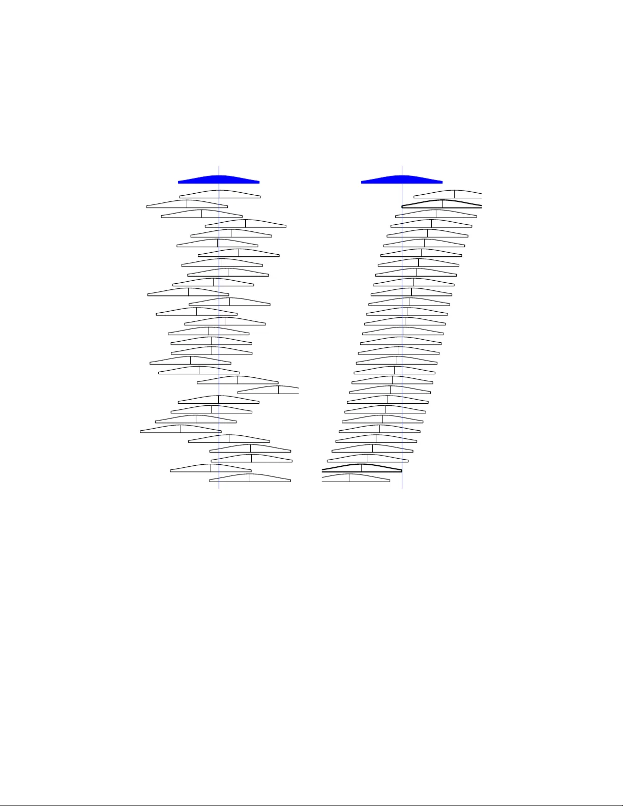
What T eac hers Should Kno w ab out the Bo otstrap: Resampling in the Undergraduate Statistics Curriculum Tim Hesterb erg Go ogle timhesterberg@gmail.com No vem b er 20, 2014 Abstract I ha ve three goals in this article: (1) T o sho w the enormous p oten tial of b ootstrapping and p erm utation tests to help studen ts understand statistical concepts including sampling distributions, standard errors, bias, conﬁdence in terv als, n ull distributions, and P -v alues. (2) T o dig deep er, understand wh y these metho ds work and when they don’t, things to w atc h out for, and how to deal with these issues when teaching. (3) T o change statistical practice—b y comparing these methods to common t tests and interv als, w e see how inaccurate the latter are; w e conﬁrm this with asymptotics. n ≥ 30 isn’t enough—think n ≥ 5000. Resampling pro vides diagnostics, and more accurate alternativ es. Sadly , the common bo otstrap p ercen tile in terv al badly under-co v ers in small samples; there are b etter alternatives. The tone is informal, with a few stories and jokes. Keywords : T eaching, b o otstrap, p erm utation test, randomization test 1 Con ten ts 1 Ov erview 3 1.1 Notation . . . . . . . . . . . . . . . . . . . . . . . . . . . . . . 4 2 In tro duction to the Bo otstrap and P ermutation T ests 5 2.1 P ermutation T est . . . . . . . . . . . . . . . . . . . . . . . . . 6 2.2 P edagogical V alue . . . . . . . . . . . . . . . . . . . . . . . . 6 2.3 One-Sample Bo otstrap . . . . . . . . . . . . . . . . . . . . . . 8 2.4 Tw o-Sample Bo otstrap . . . . . . . . . . . . . . . . . . . . . . 9 2.5 P edagogical V alue . . . . . . . . . . . . . . . . . . . . . . . . 12 2.6 T eac hing Tips . . . . . . . . . . . . . . . . . . . . . . . . . . . 13 2.7 Practical V alue . . . . . . . . . . . . . . . . . . . . . . . . . . 13 2.8 Idea b ehind Bo otstrapping . . . . . . . . . . . . . . . . . . . . 15 3 V ariation in Bo otstrap Distributions 20 3.1 Sample Mean, Large Sample Size: . . . . . . . . . . . . . . . . 20 3.2 Sample Mean: Small Sample Size . . . . . . . . . . . . . . . . 22 3.3 Sample Median . . . . . . . . . . . . . . . . . . . . . . . . . . 24 3.4 Mean-V ariance Relationship . . . . . . . . . . . . . . . . . . . 27 3.5 Summary of Visual Lessons . . . . . . . . . . . . . . . . . . . 27 3.6 Ho w many b o otstrap samples? . . . . . . . . . . . . . . . . . 28 4 T ransformation, Bias, and Skewness 31 4.1 T ransformations . . . . . . . . . . . . . . . . . . . . . . . . . 31 4.2 Bias . . . . . . . . . . . . . . . . . . . . . . . . . . . . . . . . 32 4.2.1 Bias-Adjusted Estimates . . . . . . . . . . . . . . . . . 34 4.2.2 Causes of Bias . . . . . . . . . . . . . . . . . . . . . . 34 4.3 F unctional Statistics . . . . . . . . . . . . . . . . . . . . . . . 35 4.4 Sk ewness . . . . . . . . . . . . . . . . . . . . . . . . . . . . . 37 4.5 Accuracy of the CL T and t Statistics . . . . . . . . . . . . . . 41 5 Conﬁdence In terv als 42 5.1 Conﬁdence In terv al Pictures . . . . . . . . . . . . . . . . . . . 46 5.2 Statistics 101—P ercentile, and T with Bo otstrap SE . . . . . 49 5.3 Expanded P ercentile Interv al . . . . . . . . . . . . . . . . . . 50 5.4 Rev erse Bo otstrap P ercentile Interv al . . . . . . . . . . . . . . 54 5.5 Bo otstrap T . . . . . . . . . . . . . . . . . . . . . . . . . . . . 56 5.6 Conﬁdence In terv als Accuracy . . . . . . . . . . . . . . . . . . 58 5.6.1 Asymptotics . . . . . . . . . . . . . . . . . . . . . . . 64 2 5.6.2 Sk ewness-Adjusted t T ests and Interv als . . . . . . . . 65 6 Bo otstrap Sampling Metho ds 67 6.1 Bo otstrap Regression . . . . . . . . . . . . . . . . . . . . . . . 67 6.2 P arametric Regression . . . . . . . . . . . . . . . . . . . . . . 70 6.3 Smo othed Bo otstrap . . . . . . . . . . . . . . . . . . . . . . . 70 6.4 Av oiding Narrowness Bias . . . . . . . . . . . . . . . . . . . . 71 6.5 Finite P opulation . . . . . . . . . . . . . . . . . . . . . . . . . 71 7 P ermutation T ests 71 7.1 Details . . . . . . . . . . . . . . . . . . . . . . . . . . . . . . . 72 7.2 T est of Relationships . . . . . . . . . . . . . . . . . . . . . . . 73 7.3 Limitations . . . . . . . . . . . . . . . . . . . . . . . . . . . . 76 7.4 Bo otstrap Hyp othesis T esting . . . . . . . . . . . . . . . . . . 77 8 Summary 78 1 Ov erview I fo cus in this article on how to use relatively simple bo otstrap metho ds and p erm utation tests to help students understand statistical concepts, and what instructors should know ab out these metho ds. I ha ve Stat 101 and Mathematical Statistics in mind, though the metho ds can b e used elsewhere in the curriculum. F or more background on the b ootstrap and a broader arra y of applications, see (Efron and Tibshirani, 1993; Da vison and Hinkley, 1997). Undergraduate textb o oks that consistently use resampling as to ols in their own right and to motiv ate classical metho ds are b eginning to app ear, including Lock et al. (2013) for Introductory Statistics and Chihara and Hesterb erg (2011) for Mathematical Statistics. Other texts incorp orate at least some resampling. Section 2 is an introduction to one- and tw o-sample b o otstraps and tw o- sample p erm utation tests, and how to use them to help studen ts understand sampling distributions, standard errors, bias, conﬁdence interv als, hypoth- esis tests, and P -v alues. W e discuss the idea b ehind the b o otstrap, wh y it w orks, and principles that guide our application. In Section 3 we tak e a visual approach tow ard understanding when the b ootstrap works and when it do esn’t. W e compare the eﬀect on b ootstrap distributions of t w o sources of v ariation—the original sample, and bo otstrap sampling. 3 In Section 4 we lo ok at three things that aﬀect inferences—bias, skew- ness, and transformations—and something that can cause o dd results for b ootstrapping, whether a statistic is functional. This section also discusses ho w inaccurate classical t pro cedures are when the p opulation is skew ed. I ha ve a broader goal b eyond better p edagogy—to c hange statistical practice. Resampling pro vides diagnostics, and alternatives. This leads to Section 5, on conﬁdence interv als; b eginning with a visual approac h to how conﬁdence in terv als should handle bias and skewness, then a description of diﬀerent conﬁdence in terv als pro cedures and their merits, and ﬁnishing with a discussion of accuracy , using simulation and asymp- totics. In Section 6 w e consider sampling metho ds for diﬀerent situations, in particular regression, and w ays to sample to a void certain problems. W e return to p erm utation tests in Section 7, to lo ok b ey ond the tw o- sample test to other applications where these tests do or do not apply , and ﬁnish with a short discussion of b ootstrap tests. Section 8 summarizes k ey issues. T eac hers are encouraged to use the examples in this article in their own classes. I’ll include a few bad jok es; you’re w elcome to those to o. Ex- amples and ﬁgures are created in R (R Core T eam, 2014), using the r e- sample pack age (Hesterb erg, 2014). I’ll put datasets and scripts at http: //www.timhesterberg.net/bootstrap . I suggest that all readers b egin by skimming the pap er, reading the b o xes and Figures 20 and 21, b efore returning here for a full pass. There are sections you may wish to read out of order. If y ou ha ve exp e- rience with resampling y ou may wan t to read the summary ﬁrst, Section 8. T o fo cus on p erm utation tests read Section 7 after Section 2.2. T o see a broader range of b ootstrap sampling metho ds earlier, read Section 6 after Section 2.8. And y ou may skip the Notation section, and refer to it as needed later. 1.1 Notation This section is for reference; the notation is explained when it comes up. W e write F for a p opulation, with corresponding parameter θ ; in speciﬁc applications w e ma y hav e e.g. θ = µ or θ = µ 1 − µ 2 ; the corresp onding sample estimates are ˆ θ , ¯ x , or ¯ x 1 − ¯ x 2 . ˆ F is an estimate for F . Often ˆ F is the empirical distribution ˆ F n , with probabilit y 1 /n on each observ ation in the original sample. When dra wing samples from ˆ F , the corresp onding estimates are ˆ θ ∗ , ¯ x ∗ , or ¯ x ∗ 1 − ¯ x ∗ 2 . 4 s 2 = ( n − 1) − 1 P ( x i − ¯ x ) 2 is the usual sample v ariance, and ˆ σ 2 = n − 1 P ( x i − ¯ x ) 2 = ( n − 1) s 2 /n is the v ariance of ˆ F n . When w e say “sampling distribution”, w e mean the sampling distribution for ˆ θ or ¯ X when sampling from F , unless otherwise noted. r is the num ber of resamples in a bo otstrap or p erm utation distribu- tion. The mean of the b o otstrap distribution is ˆ θ ∗ or ¯ x ∗ , and the standard deviation of the bo otstrap distribution (the b ootstrap standard error) is s B = q ( r − 1) − 1 P r i =1 ( ˆ θ ∗ i − ˆ θ ∗ ) 2 or s B = q ( r − 1) − 1 P r i =1 ( ¯ x ∗ i − ¯ x ∗ ) 2 . The t in terv al with b ootstrap standard error is ˆ θ ± t α/ 2 ,n − 1 s B . G represen ts a theoretical bo otstrap or p erm utation distribution, and ˆ G is the approximation by sampling; the α quan tile of this distribution is q α = ˆ G − 1 ( α ). The b o otstrap p ercen tile in terv al is ( q α/ 2 , q 1 − α/ 2 ), where q are quan tiles of ˆ θ ∗ . The expanded p ercen tile in terv al is ( q α 0 / 2 , q 1 − α 0 / 2 ), where α 0 / 2 = Φ( − p n/ ( n − 1) t α/ 2 ,n − 1 ). The rev erse p ercen tile in terv al is (2 ˆ θ − q 1 − α/ 2 , 2 ˆ θ − q α/ 2 ). The b o otstrap t in terv al is ( ˆ θ − q 1 − α/ 2 ˆ S , ˆ θ − q α/ 2 ˆ S ) where q are quantiles for ( ˆ θ ∗ − ˆ θ ) / ˆ S ∗ and ˆ S is a standard error for ˆ θ . Johnson’s (sk ewness-adjusted) t statistic is t 1 = t + κ (2 t 2 + 1) where κ = sk ewness / (6 √ n ). The sk ewness-adjusted t in terv al is ¯ x + ( κ (1 + 2 t 2 α/ 2 ) ± t α/ 2 )( s/ √ n ). 2 In tro duction to the Bo otstrap and P erm utation T ests W e’ll b egin with an example to illustrate the b ootstrap and p erm utation tests pro cedures, discuss p edagogical adv an tages of these pro cedures, and the idea b ehind b o otstrapping. Studen t B. R. w as anno yed b y TV commercials. He suspected that there w ere more commercials in the “basic” TV c hannels, the ones that come with a cable TV subscription, than in the “extended” channels y ou pa y extra for. T o c heck this, he collected the data sho wn in T able 1. He measured an a verage of 9.21 minutes of commercials p er half hour in the basic c hannels, vs only 6.87 minutes in the extended channels. This seems to supp ort his hypothesis. But there is not muc h data—p erhaps the diﬀerence w as just random. The p oor guy could only stand to w atc h 20 random half hours of TV. Actually , he didn’t even do that—he got his girl- 5 Basic 6.95 10.013 10.62 10.15 8.583 7.62 8.233 10.35 11.016 8.516 Extended 3.383 7.8 9.416 4.66 5.36 7.63 4.95 8.013 7.8 9.58 T able 1: Minutes of c ommer cials p er half-hour of TV. friend to w atch half of it. (Are you as appalled b y the deluge of commercials as I am? This is p er half-hour!) 2.1 P erm utation T est Ho w easy would it be for a diﬀerence of 2.34 minutes to o ccur just by c hance? T o answer this, w e supp ose there really is no diﬀerence b et w een the tw o groups, that “basic” and “extended” are just lab els. So what would happ en if we assign lab els randomly? How often would a diﬀerence like 2.34 o ccur? W e’ll p o ol all tw en ty observ ations, randomly pick 10 of them to lab el “basic” and lab el the rest “extended”, and compute the diﬀerence in means b et w een the tw o groups. W e’ll rep eat that man y times, sa y ten thousand, to get the p ermutation distribution shown in Figure 1. The observ ed statistic 2 . 34 is also shown; the fraction of the distribution to the righ t of that v alue ( ≥ 2 . 34) is the probabilit y that random lab eling w ould give a diﬀerence that large. In this case, the probabilit y , the P -v alue, is 0 . 005; it would b e rare for a diﬀerence this large to o ccur b y chance. Hence w e conclude there is a real diﬀerence b et w een the groups. W e defer some details until Section 7.1, including why we add 1 to n u- merator and denominator, and why we calculate a tw o-sided P -v alue this w ay . 2.2 P edagogical V alue This pro cedure pro vides nice visual represen tation for what are otherwise abstract concepts—a null distribution, and a P -v alue. Students can use the same to ols they previously used for lo oking at data, like histograms, to insp ect the null distribution. And it makes the conv oluted logic of h yp othesis testing quite natural. (Supp ose the null hypothesis is true, ho w often we would get a statistic this large or larger?) Students can learn that “statistical signiﬁcance” means “this result w ould rarely o ccur just by chance”. 6 Diff erence in means TV data −3 −2 −1 0 1 2 3 0.0 0.1 0.2 0.3 0.4 ● ● Obser v ed Mean Figure 1: Permutation distribution for the diﬀer enc e in me ans b etwe en b asic and extende d channels. The observed diﬀerence of 2 . 34 is sho wn; a fraction 0 . 005 of the distribution is to the right of that v alue ( ≥ 2 . 34). Tw o-Sample Perm utation T est P o ol the n 1 + n 2 v alues rep eat 9999 times Dra w a resample of size n 1 without replacemen t. Use the remaining n 2 observ ations for the other sample. Calculate the diﬀerence in means, or another statistic that com- pares samples. Plot a histogram of the random statistic v alues; show the observed statistic. Calculate the P -v alue as the fraction of times the random statis- tics exceed or equal the observed statistic (add 1 to numerator and denominator); m ultiply by 2 for a t wo-sided test. 7 It has the adv an tage that students can work directly with the statistic of interest—the diﬀerence in means—rather than switching to some other statistic lik e a t statistic. It generalizes nicely to other statistics. W e could w ork with the diﬀerence in medians, for example, or a diﬀerence in trimmed means, without needing new form ulas. P edagogical V alue of Tw o-Sample Perm utation T est • Mak e abstract concepts concrete—null distribution, P -v alue. • Use familiar to ols, like histograms. • W ork with the statistic of in terest, e.g. diﬀerence of means. • Generalizes to other statistics, don’t need new formulas. • Can c heck answers obtained using formulas. 2.3 One-Sample Bo otstrap In addition to using the p erm utation test to see whether there is a diﬀer- ence, we can also use resampling, in particular the b o otstrap, to quan tify the random v ariabilit y in the t wo sample estimates, and in the estimated diﬀerence. W e’ll start with one sample at a time. In the b o otstrap, we dra w n observ ations with replacement from the orig- inal data to create a b o otstr ap sample or r esample , and calculate the mean for this resample. W e rep eat that man y times, say 10000. The b ootstrap means comprise the b o otstr ap distribution . The b o otstrap distribution is a sampling distribution , for ˆ θ ∗ (with sam- pling from the empirical distribution); w e’ll talk more b elow ab out how it relates to the sampling distribution of ˆ θ (sampling from the p opulation F ). (In the sequel, when we sa y “sampling distribution” we mean the latter, not the b ootstrap distribution, unless noted.) Figure 2 shows the b ootstrap distributions for the Basic and Extended data. F or each distribution, we lo ok at the center, spread, and shap e: cen ter: Each distribution is centered approximately at the observed statis- tic; this indicates that the sample mean is approximately unbiased for the p opulation mean. W e discuss bias in Section 4.2. 8 spread: The spread of each distribution estimates how muc h the sample mean v aries due to random sampling. The b o otstr ap standar d err or is the sample standard deviation of the b ootstrap distribution, shap e: Each distribution is approximately normally distributed. A quick-and-dirt y conﬁdence interv al, the b o otstr ap p er c entile c onﬁdenc e in- terval , is the range of the middle 95% of the b ootstrap distribution; this is (8 . 38 , 9 . 99) for the Basic c hannels and (5 . 61 , 8 . 06) for the Extended c han- nels. (Cav eat—p ercen tile interv als are to o short in samples this small, see Sections 3.2 and 5.2, and Figures 20 – 22). Here are the summaries of the b o otstrap distributions for basic and ex- tended c hannels Summary Statistics: Observed SE Mean Bias Basic 9.21 0.4159658 9.207614 -0.002386 Observed SE Mean Bias Extended 6.87 0.6217893 6.868101 -0.001899 The spread for Extended is larger, due to the larger standard deviation in the original data. Here, and elsewhere unless noted, w e use 10 4 resamples for the b ootstrap or 10 4 − 1 for p ermutation tests. 2.4 Tw o-Sample Bo otstrap F or a t w o-sample b ootstrap, we independently draw bo otstrap samples from eac h sample, and compute the statistic that compares the samples. F or the TV commercials data, w e dra w a sample of size 10 from Basic data, an- other sample of size 10 from the Extended data, and compute the diﬀerence in means. The resulting b o otstrap distribution is shown in Figure 3. The mean of the distribution is very close to the observed diﬀerence in means, 2 . 34; the b o otstrap standard error is 0 . 76, and the 95% b ootstrap p ercen tile conﬁdence interv al is (0 . 87 , 3 . 84). The interv al do es not include zero, which suggests that the diﬀerence b et ween the samples is larger than can b e ex- plained by random v ariation; this is consistent with the p ermutation test ab o v e. Recall that for the p erm utation test w e resampled in a wa y that was consisten t with the n ull h yp othesis of no diﬀerence betw een p opulations, and the p erm utation distribution for the diﬀerence in means was centered at zero. Here w e mak e no such assumption, and the b o otstrap distribution 9 Commercial Time (Basic) Density 5 6 7 8 9 10 0.0 0.2 0.4 0.6 0.8 1.0 ● ● Observed Mean −4 −2 0 2 4 8.0 8.5 9.0 9.5 10.0 Normal Q−Q Plot Theoretical Quantiles Commercial Time (Basic) Commercial Time (Extended) Density 5 6 7 8 9 10 0.0 0.1 0.2 0.3 0.4 0.5 0.6 0.7 ● ● Observed Mean −4 −2 0 2 4 5 6 7 8 9 Normal Q−Q Plot Theoretical Quantiles Commercial Time (Extended) Figure 2: Bo otstr ap distributions for TV data. Bo otstrap distributions for the mean of the basic channels (top) and extended channels (b ottom). The observ ed v alues, and means of the b o otstrap distributions, are sho wn. These are sampling distributions for ¯ x ∗ 1 and ¯ x ∗ 2 . 10 One-Sample Bo otstrap rep eat r = 10000 times Dra w a sample of size n with replacement from the original data (a b o otstr ap sample or r esample ). Compute the sample mean (or other statistic) for the resample. The 10000 b ootstrap statistics comprise the b o otstr ap distribution . Plot the b ootstrap distribution. The b o otstr ap standar d err or is the standard deviation of the b oot- strap distribution, s B = q P ( ˆ θ ∗ i − ˆ θ ∗ ) 2 / ( r − 1). The b o otstr ap p er c entile c onﬁdenc e interval is the range of the middle 95% of the b ootstrap distribution. The b o otstr ap bias estimate is mean of the b o otstrap distribution, min us the observed statistic, ˆ θ ∗ − ˆ θ . Diff erence in means Density 0 1 2 3 4 5 0.0 0.1 0.2 0.3 0.4 0.5 ● ● Observed Mean −4 −2 0 2 4 0 1 2 3 4 5 Normal Q−Q Plot Theoretical Quantiles Diff erence in means Figure 3: Two-sample b o otstr ap for TV c ommer cials data. Bo otstrap dis- tribution for the diﬀerence of means b et ween extended and basic channels. This is the sampling distribution of ¯ x ∗ 1 − ¯ x ∗ 2 . 11 is centered at the observed statistic; this is used for conﬁdence interv als and standard errors. 2.5 P edagogical V alue Lik e p erm utation tests, the b ootstrap mak es the abstract concrete. Con- cepts like sampling distributions, standard errors, bias, central limit theo- rem, and conﬁdence in terv als are abstract, and hard for many studen ts, and this is usually comp ounded by a scary co okbo ok of form ulas. The b o otstrap pro cess, in volving sampling, reinforces the central role that sampling from a p opulation pla ys in statistics. Sampling v ariabilit y is visible, and it is natural to measure the v ariability of the b ootstrap distribu- tion using the interquartile range or the standard deviation; the latter is the b ootstrap standard error. Students can see if the sampling distribution has a b ell-shaped curve. It is natural to use the middle 95% of the distribution as a 95% conﬁdence in terv al. Studen ts can obtain the conﬁdence in terv al by w orking directly with the statistic of interest, rather than using a t statistic. The b ootstrap works the same w ay with a wide v ariet y of statistics. This makes it easy for students to w ork with a v ariet y of statistics without needing to memorize more formulas. The b ootstrap can also reinforce the understanding of form ula metho ds, and provide a wa y for students to chec k their work. Studen ts may kno w the formula s/ √ n without understanding what it really is; but they can compare it to the b o otstrap standard error, and see that it measures how the sample mean v aries due to random sampling. The bo otstrap lets us do b etter statistics. In Stat 101 w e talk early on ab out means and medians for summarizing data, but ignore the median later, lik e a crazy uncle hidden aw a y in a closet, b ecause there are no easy form ulas for conﬁdence interv als. Studen ts can b o otstrap the median or trimmed mean as easily as the mean. W e can use robust statistics when appropriate, rather than only using the mean. Y ou do not need to talk ab out t statistics and t interv als at all, though y ou will undoubtedly wan t to do so later. At that p oin t y ou ma y introduce another quick-and-dirt y conﬁdence in terv al, the t interval with b o otstr ap standar d err or , ˆ θ ± t α/ 2 s B where s B is the b o otstrap standard error. (This is not to b e confused with the b o otstr ap t interval , see Section 5.5.) 12 P edagogical V alue of the Bo otstrap • Mak e abstract concepts concrete—sampling distribution, stan- dard error, bias, cen tral limit theorem. • The pro cess mimics the role of random sampling in real life. • Use familiar to ols, like histograms and normal quantile plots. • Easy , intuitiv e conﬁdence interv al—b ootstrap p ercen tile inter- v al. • W ork with the statistic of in terest, e.g. diﬀerence of means. • Generalizes to other statistics, don’t need new formulas. • Can c heck answers obtained using formulas. 2.6 T eaching Tips F or b oth b o otstrapping and p erm utation tests, start small, and let students do some samples b y hand. F or permutation tests, starting with small groups lik e 2 and 3 allows studen ts to do all  n n 1  partitions exhaustiv ely . There is a nice visualization of the pro cess of p erm utation testing as part of the iNZigh t pac k age < https://www.stat.auckland.ac.nz/ ~ wild/ iNZight> . It demonstrates the whole pro cess: po oling the data, then re- p eatedly randomly splitting the data and calculating a test statistic, to build up the p erm utation distribution. 2.7 Practical V alue Resampling is also imp ortan t in practice, often providing the only practical w ay to do inference. I’ll giv e some examples from Go ogle, from my w ork or others. In Go ogle Search w e estimate the av erage num b er of words p er query , in ev ery country (Chamandy, 2014). The data is immense, and is “sharded”— stored on tens of thousands of mac hines. W e can count the n um b er of queries in each country , and the total num b er of words in queries in each coun try , b y coun ting on eac h mac hine and adding across mac hines, using MapReduce (Dean and Ghemaw at, 2008). But w e also wan t to estimate the v ariance, for users in eac h coun try , in w ords p er query p er user. The queries for each user are sharded, and it is not feasible to calculate queries and w ords for ev ery user. But there is a b ootstrap pro cedure we can use. In the ordinary 13 b ootstrap, the n umber of times each observ ation is included in a b o otstrap sample is Binomial( n, 1 /n ), which we approximate as P oisson(1). F or each user, we generate r Poisson v alues, one for each resample. W e don’t actually sa ve these, instead they are generated on the ﬂy , eac h time the user comes up on any machine, using a random n umber seed generated from the user’s co okie, so the user gets the same num b ers each time. W e then compute w eighted counts using the P oisson weigh ts, to estimate the v ariance across users of w ords p er query . Also in Searc h, we contin ually run h undreds of exp eriments, trying to impro ve search results, sp eed, usability , and other factors; each year there are thousands of exp erimen ts resulting in h undreds of improv ements 1 (when y ou search on Go ogle y ou are probably in a dozen or more exp erimen ts). The data are sharded, and we cannot combine results for each user. W e split the users into 20 groups, and analyze the v ariabilit y across these groups using the jac kknife (another resampling technique). In Br and Lift 2 w e use designed exp erimen ts to estimate the eﬀectiveness of displa y advertisemen ts. W e ask p eople brand a wareness questions suc h as whic h brands they are familiar with, to see whether the exp osed (treatmen t) and con trol groups diﬀer. There are four nested p opulations: (1) p eople who sa w an ad (and con trol sub jects who would ha ve seen one), (2) those eligible for solicitation (they visit a website where the surv ey can b e presented), (3) those randomly selected for solicitation, (4) resp onden ts. W e use t wo logistic regression mo dels: (A) data = (4), Y = actual resp onse, (B) data = (4,3), Y = actual resp onse or predictions from (A), with X ’s such as age and gender to correct for random diﬀerences in these co v ariates b et ween exp osed and controls. W e use predictions from mo del (A) to extrap olate to (2–3), and predictions from mo del (B) to extrap olate to (1). The estimated a v erage ad eﬀect is the diﬀerence, across exp osed p eople, of ˆ p 1 − ˆ p 0 , where ˆ p 1 = ˆ P ( Y = 1 | x ) is the usual prediction, and ˆ p 0 = ˆ P ( Y = 1 | x except set to con trol) is the prediction if the person w ere a con trol. F orm ula standard errors for this pro cess are theoretically p ossible but diﬃcult to deriv e, and would need up dating when we c hange the mo del; w e b o otstrap instead. 1 http://www.businessweek.com/the_thread/techbeat/archives/2009/10/google_ search_g.html 2 https://www.thinkwithgoogle.com/products/brand- lift.html . Chan et al. (2010) describ e an earlier version. 14 F or the People Analytics gDNA 3 longitudinal surv ey , w e use 5-fold cross- v alidation (another resampling tec hnique) to ev aluate a messy v ariable se- lection routine: m ultiple-imputation follo wed by bac kw ard-elimination in a linear mixed eﬀects mo del. The mo dels pro duced within eac h fold giv e an indication of the stabilit y of the ﬁnal result, and we calculate precision, recall, and accuracy on the holdout sets. 2.8 Idea b ehind Bo otstrapping A t this p oint you may hav e a million questions, but foremost among them is probably: wh y do es this work? W e’ll address that next b y talking ab out the k ey idea b ehind the b ootstrap, saving other questions for later. Muc h of inferential statistics requires estimating something ab out the sampling distribution, e.g. standard error is an estimate of the standard deviation of that distribution. In principle, the sampling distribution is obtained b y • Dra w samples from the p opulation . • Compute the statistic of in terest for each sample (such as the mean, median, etc.) • The distribution of the statistics is the sampling distribution . This is sho wn in Figure 4. The problem with this is that w e cannot draw arbitrarily many samples from the p opulation—it is to o expensive, or infeasible b ecause we don’t kno w the p opulation. Instead, w e hav e only one sample. The b ootstrap idea is to draw samples from an estimate of the p opulation, in lieu of the p opulation: • Dra w samples from an estimate of the p opulation. • Compute the statistic of in terest for each sample. • The distribution of the statistics is the b o otstr ap distribution . This is sho wn in Figure 5. Plug-in Principle The b ootstrap is based on the plug-in principle —if something is unknown, then substitute an estimate for it. This principle is v ery familiar to statisticians. F or example, the v ariance for the sample mean is σ / √ n ; when σ is unknown we substitute an estimate s , the sample standard deviation. With the bo otstrap w e tak e this one step farther— instead of plugging in an estimate for a single parameter, we plug in an estimate for the whole distribution. 3 http://blogs.hbr.org/2014/03/googles- scientific- approach- to- work- life- balance- and- much- more/ 15 −6 8 µ −6 8 x µ Density −6 8 x Density −6 8 x Density −6 8 x Density −6 8 x x −3 3 µ P opulation F Sampling distribution of θ ^ = x Samples Figure 4: Ide al world. Sampling distributions are obtained b y drawing rep eated samples from the p opulation, computing t he statistic of interest for eac h, and collecting (an inﬁnite num ber of ) those statistics as the sampling distribution. 16 Density −6 8 x x µ −6 8 x * x Density −6 8 x * Density −6 8 x * Density −6 8 x * Density −6 8 x * x * −3 3 µ x Estimate of population= original data F ^ Bootstrap distribution of θ ^ * = x * Bootstrap Samples Figure 5: Bo otstr ap world. The b ootstrap distribution is obtained b y dra wing rep eated samples from an estimate of the p opulation, computing the statistic of interest for eac h, and collecting those statistics. The distribution is cen tered at the observed statistic ( ¯ x ), not the parameter ( µ ). 17 What to Substitute This raises the question of what to substitute for F . Possibilities include: Nonparametric b o otstrap: The common bo otstrap pro cedure, the non- p ar ametric b o otstr ap , consists of dra wing samples from the empirical distribution ˆ F n (with probabilit y 1 /n on eac h observ ation), i.e. draw- ing samples with replacement from the data. This is the primary fo cus of this article. Smo othed Bo otstrap: When w e b eliev e the p opulation is contin uous, w e may draw samples from a smo oth p opulation, e.g. from a kernel densit y estimate of the p opulation. P arametric Bo otstrap: In parametric situations w e ma y estimate pa- rameters of the distribution(s) from the data, then draw samples from the parametric distribution(s) with those parameters. W e discuss these and other metho ds below in Section 6. F undamen tal Bo otstrap Principle The fundamental b ootstrap princi- ple is that this substitution works. In most cases, the b o otstrap distribution tells us something useful ab out the sampling distribution. There are some things to watc h out for, wa ys that the b o otstrap distri- bution cannot b e used for the sampling distribution. W e discuss some of these b elo w, but one is imp ortan t enough to mention immediately: Inference, Not Better Estimates The b o otstr ap distribution is c enter e d at the observe d statistic, not the p opulation p ar ameter , e.g. at ¯ x , not µ . This has tw o profound implications. First, it m eans that we do not use the bo otstrap to get b etter estimates 4 . F or example, w e cannot use the b ootstrap to improv e on ¯ x ; no matter ho w many bo otstrap samples w e take, they are alwa ys cen tered at ¯ x , not µ . W e’d just b e adding random noise to ¯ x . Instead we use the b ootstrap to tell how accurate the original estimate is. Some p eople are suspicious of the bo otstrap, b ecause they think the b ootstrap creates data out of nothing. (The name “b o otstrap” doesn’t help, 4 There are exceptions, where the b o otstrap is used to obtain b etter estimates, for example in random forests. These are typically where a b o otstrap-lik e pro cedure is used to work around a ﬂaw in the basic pro cedure. F or example, consider estimating E ( Y | X = x ) where the true relationship is smo oth, but you are limited to using a step function with relatively few steps. By taking bo otstrap samples and applying the step function estimation pro cedure to each, the step b oundaries v ary b et ween samples; by av eraging across samples the few large steps are replaced by many smaller ones, giving a smo other estimate. This is b agging (b ootstrap aggregating). 18 since it implies creating something out of nothing.) The b o otstrap do esn’t create all those b o otstrap samples and use them as if they were more real data; instead it uses them to tell how accurate the original estimate is. In this regard it is no diﬀerent than form ula metho ds that use the data t wice—once to compute an estimate, and again to compute a standard error for the estimate. The b o otstrap just uses a diﬀerent approach to estimating the standard error. The second implication is that we do not use quantiles of the b ootstrap distribution of ˆ θ ∗ to estimate quan tiles of the sampling distribution of ˆ θ . Instead, we use the b ootstrap distribution to estimate the standard devia- tion of the sampling distribution, or the exp ected v alue of ˆ θ − θ . Later, in Sections 5.4 and 5.5, w e will use the b o otstrap to estimate quantiles of ˆ θ − θ and ( ˆ θ − θ ) / SE. Second Bo otstrap Principle The second b o otstrap principle is to sam- ple with replacemen t from the data. Actually , this isn’t a principle at all, but an implementation detail. W e ma y sample from a parametric distribution, for example. And ev en for the nonparametric b o otstrap, w e sometimes a void random sampling. There are n n p ossible samples, or  2 n − 1 n  if order do esn’t matter; if n is small we could ev aluate all of these. In some cases, like binary data, the n umber of unique samples is smaller. W e’ll call this a the or etic al b o otstr ap or exhaustive b o otstr ap . But more often this is infeasible, so we dra w say 10000 random samples instead; w e call this the Monte Carlo implementation or sampling implementation . W e talk ab out how many samples to dra w in Section 3.6. Ho w to Sample Normally we should draw b ootstrap samples the same w ay the sample was drawn in real life, e.g. simple random sampling, stratiﬁed sampling, or ﬁnite-p opulation sampling. There are exceptions to that rule, see Section 6. One is imp ortan t enough to mention here—to c ondition on the observe d information . F or example, when comparing samples of size n 1 and n 2 , we ﬁx those num b ers, ev en if the original sampling pro cess could hav e pro duced diﬀeren t counts. W e can also mo dify the sampling to answer what-if questions. Supp ose the original sample size w as 100, but w e dra w samples of size 200. That estimates what would happ en with samples of that size—how large stan- dard errors and bias w ould b e, and how wide conﬁdence in terv als would b e. (W e would not actually use the conﬁdence in terv als from this proc ess as 19 real conﬁdence interv als; they would imply more precision than our sample of 100 pro vides.) Similarly , w e can b o otstrap with and without stratiﬁca- tion and compare the resulting standard errors, to in vestigate the v alue of stratiﬁcation. Hyp othesis testing is another what-if question—if the p opulation satisﬁes H 0 , what w ould the sampling distribution (the null distribution) lo ok like? W e ma y b o otstrap in a wa y that matc hes H 0 , b y mo difying the p opulation or the sampling metho d; see Section 7.4. Idea Behind the Bo otstrap The idea behind the b ootstrap is to estimate the p opulation, then dra w samples from that estimate, normally sampling the same wa y as in real life. The resulting b o otstr ap distribution is an estimate of the sampling distribution. W e use this for inferences, not to obtain better estimates. It is centered at the statistic (e.g. ¯ x ) not the parameter ( µ ). 3 V ariation in Bo otstrap Distributions I claimed ab o ve that the b o otstrap distribution usually tells us something useful ab out the sampling distribution, with exceptions. I elab orate on that no w with a series of visual examples, starting with one where things generally w ork well, and three with problems. The examples illustrate t wo questions: • Ho w accurate is the theoretical (exhaustive) b o otstrap? • Ho w accurately do es the Monte Carlo implemen tation appro ximate the theoretical b ootstrap? Both reﬂect random v ariation: • The original sample is c hosen randomly from the p opulation. • Bo otstrap resamples are chosen randomly from the original sample. 3.1 Sample Mean, Large Sample Size: Figure 6 shows a p opulation and ﬁve samples of size 50 from the p opulation in the left column. The middle column shows the sampling distribution for the mean and b o otstrap distributions from each sample, based on r = 10 4 b ootstrap samples. Each b o otstrap distribution is cen tered at the statistic 20 −3 8 µ P opulation −3 8 x Sample 1 −3 8 x Sample 2 −3 8 x Sample 3 −3 8 x Sample 4 −3 8 x Sample 5 0 4 µ Sampling Distribution of x ● 0 4 x Bootstrap distribution from sample 1 of x * ● 0 4 x Bootstrap distribution from sample 2 of x * ● 0 4 x Bootstrap distribution from sample 3 of x * ● 0 4 x Bootstrap distribution from sample 4 of x * ● 0 4 x Bootstrap distribution from sample 5 of x * ● 0 4 x Bootstrap distribution from sample 1 R = 1000 ● 0 4 x Bootstrap distribution from sample 1 R = 1000 ● 0 4 x Bootstrap distribution from sample 1 R = 1000 ● 0 4 x Bootstrap distribution from sample 1 R = 10000 ● 0 4 x Bootstrap distribution from sample 1 R = 10000 ● 0 4 x Bootstrap distribution from sample 1 R = 10000 Figure 6: Bo otstr ap distribution for the me an, n = 50 . The left col- umn sho ws the p opulation and ﬁv e samples. The middle column shows the sampling distribution for ¯ X , and b ootstrap distributions of ¯ X ∗ from each sample, with r = 10 4 . The righ t column sho ws more b ootstrap distributions from the ﬁrst sample, three with r = 1000 and three with r = 10 4 . 21 ( ¯ x ) from the corresp onding sample rather than b eing centered at the p opu- lation mean µ . The spreads and shap es of the b ootstrap distributions v ary a bit but not a lot. This informs what the bo otstrap distributions ma y b e used for. The b ootstrap do es not provide a b etter estimate of the p opulation parameter, b ecause no matter how many b ootstrap samples are used, they are centered at ¯ x , not µ . Instead, the b ootstrap distributions are useful for estimating the spread and shap e of the sampling distribution. The righ t column sho ws additional b o otstrap distributions from the ﬁrst sample, with r = 1000 or r = 10 4 resamples. Using more resamples re- duces random Monte Carlo v ariation, but do es not fundamentally c hange the bo otstrap distribution—it still has the same approximate center, spread, and shap e. The Mon te Carlo v ariation is muc h smaller than the v ariation due to diﬀeren t original samples. F or many uses, suc h as quic k-and-dirt y estimation of standard errors or appro ximate conﬁdence in terv als, r = 1000 resamples is adequate. Ho wev er, there is noticeable v ariabilit y , particularly in the tails of the b o otstrap distributions, so when accuracy matters, r = 10 4 or more samples should b e used. 3.2 Sample Mean: Small Sample Size Figure 7 is similar to Figure 6, but for a smaller sample size, n = 9 (and a diﬀerent p opulation). As b efore, the b o otstrap distributions are centered at the corresp onding sample means, but no w the spreads and shapes of the b ootstrap distributions v ary substan tially , b ecause the spreads and shap es of the samples v ary substantially . As a result, b o otstrap conﬁdence interv al widths v ary substantially (this is also true of non-b ootstrap conﬁdence in- terv als). As b efore, the Monte Carlo v ariation is small and may b e reduced with more samples. While not apparent in the pictures, b o otstrap distributions tend to b e to o narrow, by a factor of p ( n − 1) /n for the mean; the theoretical b o ot- strap standard error is s B = ˆ σ / √ n = p ( n − 1) /n ( s/ √ n ). The reason for this go es back to the plug-in principle; the empirical distribution has v ari- ance V ar ˆ F ( X ) = ˆ σ 2 = (1 /n ) P ( x i − ¯ x ) 2 , not s 2 . F or example, the b o otstrap standard error for the TV Basic mean is 0 . 416, while s/ √ 10 = 0 . 441. In tw o-sample or stratiﬁed sampling situations, this narr owness bias de- p ends on the individual sample or strata sizes, not the com bined size. This can result in severe narrowness bias. F or example, the ﬁrst b oots trap short course I ever taught w as for the U.K. Department of W ork and Pensions, 22 −6 6 µ P opulation −6 6 x Sample 1 −6 6 x Sample 2 −6 6 x Sample 3 −6 6 x Sample 4 −6 6 x Sample 5 −3 3 µ Sampling Distribution of x ● −3 3 x Bootstrap distribution from sample 1 of x * ● −3 3 x Bootstrap distribution from sample 2 of x * ● −3 3 x Bootstrap distribution from sample 3 of x * ● −3 3 x Bootstrap distribution from sample 4 of x * ● −3 3 x Bootstrap distribution from sample 5 of x * ● −3 3 x Bootstrap distribution from sample 1 R = 1000 ● −3 3 x Bootstrap distribution from sample 1 R = 1000 ● −3 3 x Bootstrap distribution from sample 1 R = 1000 ● −3 3 x Bootstrap distribution from sample 1 R = 10000 ● −3 3 x Bootstrap distribution from sample 1 R = 10000 ● −3 3 x Bootstrap distribution from sample 1 R = 10000 Figure 7: Bo otstr ap distributions for the me an, n = 9 . The left column sho ws the p opulation and ﬁve samples. The middle column sho ws the sam- pling distribution for ¯ X , and b o otstrap distributions of ¯ X ∗ from each sample, with r = 10 4 . The right column shows more b ootstrap distributions from the ﬁrst sample, three with r = 1000 and three with r = 10 4 . 23 who w anted to b o otstrap a survey they had p erformed to estimate welfare c heating. They used a stratiﬁed sampling pro cedure that resulted in tw o sub jects in each stratum—then the b o otstrap standard error would b e to o small by a factor of p 1 / 2. There are remedies, see Section 6. F or Stat 101 I recommend warning students ab out the issue; for higher courses y ou may discuss the remedies. The narrowness bias and the v ariabilit y in spread aﬀect conﬁdence in- terv al cov erage badly in small samples, see Section 5.2. 3.3 Sample Median No w turn to Figure 8 where the statistic is the sample median. Here the b ootstrap distributions are p oor approximations of the sampling distribu- tion. The sampling distribution is contin uous, but the b o otstrap distribu- tions are discrete—since n is odd, the b ootstrap sample median is alw a ys one of the original data p oin ts. The b o otstrap distributions are v ery sensitiv e to the sizes of gaps among the observ ations near the cen ter of the sample. The ordinary b o otstrap tends not to work well for statistics suc h as the median or other quantiles in small samples, that dep end hea vily on a small n umber of observ ations out of a larger sample; the b o otstrap distribution in turn dep ends heavily on a small num b er of observ ations (though diﬀerent ones in diﬀerent b o otstrap samples, so b o otstrapping the median of large samples works OK). The shap e and scale of the b ootstrap distribution may b e very diﬀerent than the sampling distribution. Curiously , in spite of the ugly b o otstrap distribution, the b ootstrap p er- cen tile in terv al for the median is not bad (Efron, 1982). F or odd n , percentile in terv al endp oin ts fall on one of the observ ed v alues. Exact interv al end- p oin ts also fall on one of the observed v alues (order statistics), and for a 95% interv al those are typically the same or adjacent order statistics as the p ercen tile in terv al. The right column sho ws the use of a smo othe d b o otstr ap (Silverman and Y oung, 1987; Hall et al. , 1989), drawing samples from a density estimate based on the data, rather than dra wing from the data itself. See Section 6.3. It impro ves things somewhat, though it is still not great. The b ootstrap fails altogether for estimating the sampling distribution for max( x ). 24 −3 9 M P opulation median = M Sample 1 m Sample 2 m Sample 3 m Sample 4 m Sample 5 m −3 9 M Sampling distribution of median m with n = 15 xt −3 9 m Bootstrap distribution from sample 1 xt −3 9 m Bootstrap distribution from sample 2 xt −3 9 m Bootstrap distribution from sample 3 xt −3 9 m Bootstrap distribution from sample 4 xt −3 9 m Bootstrap distribution from sample 5 Smoothed Bootstrap ● −3 9 m Smoothed bootstrap distribution from sample 1 ● −3 9 m Smoothed bootstrap distribution from sample 2 ● −3 9 m Smoothed bootstrap distribution from sample 3 ● −3 9 m Smoothed bootstrap distribution from sample 4 ● −3 9 m Smoothed bootstrap distribution from sample 5 Figure 8: Bo otstr ap distributions for the me dian, n = 15 . The left col- umn sho ws the p opulation and ﬁv e samples. The middle column shows the sampling distribution, and b ootstrap distributions from each sample, with r = 10 4 . The right column shows smo othed b ootstrap distributions, with k ernel sd s/ √ n and r = 10 4 . 25 µ P opulation 0 6 x µ Sample 1 0 6 x µ Sample 2 0 6 x µ Sample 3 0 6 x µ Sample 4 0 6 x µ Sample 5 µ Sampling Distribution ● x 0 Bootstrap distribution for sample 1 ● x 0 Bootstrap distribution for sample 2 ● x 0 Bootstrap distribution for sample 3 ● x 0 Bootstrap distribution for sample 4 ● x 0 Bootstrap distribution for sample 5 P opulation mean = µ Sample mean = x −4 −2 0 2 4 Quantiles Mean Bootstrap t distribution for sample 1 −4 −2 0 2 4 Quantiles Mean Bootstrap t distribution for sample 2 −4 −2 0 2 4 Quantiles Mean Bootstrap t distribution for sample 3 −4 −2 0 2 4 Quantiles Mean Bootstrap t distribution for sample 4 −4 −2 0 2 4 Quantiles Mean Bootstrap t distribution for sample 5 Figure 9: Bo otstr ap distributions for the me an, n = 50 , exp onential p op- ulation. The left column shows the p opulation and ﬁv e samples. (These samples are selected from a larger set of random samples, to hav e means spread across the range of sample means, and av erage standard deviations conditional on the means.) The middle column shows the sampling distri- bution and b o otstrap distributions from each sample. The thinner curv es in the top tw o ﬁgures are p opulations and sampling distributions with means equal to the sample means. Each b ootstrap distribution is lik e the sampling distribution with µ set to matc h ¯ x . The right column sho ws b ootstrap t distributions. 26 3.4 Mean-V ariance Relationship In man y applications, the spread or shap e of the sampling distribution de- p ends on the parameter of interest. F or example, the binomial distribution spread and shap e dep end on p . Similarly , for the mean from an exp onential distribution, the standard deviation of the sampling distribution is prop or- tional to the p opulation mean. This is reﬂected in b ootstrap distributions. Figure 9 shows samples and b ootstrap distributions from an exp onential p opulation. There is a strong dep endence b et ween ¯ x and the corresp onding bo otstrap SE. This has important implications for conﬁdence in terv als; go od conﬁdence in terv als need to reac h many (short) SE’s to the right to a void missing θ to o often in that direction, and should reach fewer (long) SE’s to the left. W e discuss this more in Section 5. This mean-v ariance relationship in samples normally corresp onds to a similar mean-v ariance relationship b et ween the parameter and v ariance of the sampling distribution. F or example, see the ﬁve sampling distributions in the top middle of Figure 9. W e call such a relationship ac c eler ation . The right column of Figure 9 shows b ootstrap distributions of the t statis- tic, deﬁned in Section 5.5. These distributions are m uch less sensitive to the original sample. There are other applications where sampling distributions dep end strongly on the parameter; for example sampling distributions for chi-squared statis- tics dep end on the non-cen trality parameter. Similarly for statistics for es- timating the num b er of mo des of a p opulation Use caution when b ootstrap- ping in these applications; the b o otstrap distribution may b e very diﬀerent than the sampling distribution. 3.5 Summary of Visual Lessons The bo otstrap distribution reﬂects the original sample. If the sample is narro wer than the p opulation, the b o otstrap distribution is narrow er than the sampling distribution. T ypically for large samples the data represent the p opulation w ell; for small samples they ma y not. Bo otstrapping does not ov ercome the weakness of small samples as a basis for inference. Indeed, for the very smallest samples, you ma y not w ant to b ootstrap; it ma y b e b etter to mak e additional assumptions s uc h as smo othness or a parametric family . When there is a lot of data (sampled randomly from a p opulation) we can trust the data to represent the shap e and spread of the 27 p opulation; when there is little data we cannot. Visual Lessons ab out Bo otstrap Distributions The b ootstrap distribution reﬂects the data. F or large samples the data represen t the p opulation w ell; for small samples they ma y not. The b o otstrap ma y w ork p oorly when the statistic, and sampling dis- tribution, dep end on a small num b er of observ ations. Using more bo otstrap samples reduces the v ariabilit y of bo otstrap dis- tributions, but do es not fundamentally c hange the center, spread, or shap e of the b o otstrap distribution. Lo oking ahead, tw o things matter for accurate inferences: • ho w close the b o otstrap distribution is to the sampling distribution (in this regard, the b o otstrap t has an adv an tage, judging from Figure 9); • some pro cedures b etter allow for the fact that there is v ariation in samples. F or example, the usual formula t tests and in terv als allow for v ariation in s by using t α/ 2 in place of z α ; we discuss a b o otstrap analog in Section 5.3. It app ears that the b o otstrap resampling pro cess using 1000 or more resamples introduces little additional v ariation, but for go od accuracy use 10000 or more. Let’s consider this issue more carefully . 3.6 Ho w many b o otstrap samples? W e suggested ab o ve that using 1000 b ootstrap samples for rough approx- imations, or 10 4 or more for b etter accuracy . This is ab out Mon te Carlo accuracy—ho w w ell the usual random sampling implemen tation of the bo ot- strap appro ximates the theoretical b o otstrap distribution. A b o otstrap distribution based on r random samples corresp onds to dra wing r observ ations with replacemen t from the theoretical b ootstrap dis- tribution. Brad Efron, inv entor of the b ootstrap, suggested in 1993 that r = 200, or even as few as r = 25, suﬃces for estimating standard errors and that r = 1000 is enough for conﬁdence interv als (Efron and Tibshirani, 1993). W e argue that more resamples are appropriate, on t wo grounds. First, those criteria w ere developed when computers w ere muc h slo wer; with faster computers it is easier to take more resamples. 28 Second, those criteria were developed using argumen ts that combine the random v ariation due to the original random sample with the extra v ariation due to the Mon te Carlo implemen tation. W e prefer to treat the data as giv en and lo ok just at the v ariability due to the implemen tation. Data is v aluable, and computer time is cheap. Two p eople analyzing the same data should not get substan tially diﬀerent answers due to Mon te Carlo v ariation. Quan tify accuracy b y formulas or b ootstrapping W e can quan tify the Mon te Carlo error in tw o w ays—using formulas, or by b ootstrapping. F or example, in permutation testing w e need to estimate the fraction of observ ations that exceed the observ ed v alue; the Mon te Carlo standard error is approximately p ˆ p (1 − ˆ p ) /r , where ˆ p is the estimated prop ortion. (It is a bit more complicated b ecause w e add 1 to the numerator and denominator, but this is close.) In b o otstrapping, the bias estimate dep ends on ˆ θ ∗ , a sample av erage of r v alues; the Monte Carlo standard error for this is s B / √ r where s B is the sample standard deviation of the b ootstrap distribution. W e can also bo otstrap the b o otstrap! W e can treat the r b o otstrap repli- cates like any old sample, and b ootstrap from that sample. F or example, to estimate the Mon te Carlo SE for the 97.5% quantile of the b ootstrap dis- tribution (the endp oin t of a b ootstrap p ercen tile interv al), we dra w samples of size r from the r observ ed v alues in the b ootstrap distribution, compute the quan tile for each, and tak e the standard deviation of those quan tiles as the Mon te Carlo SE. F or example, the 95% p ercen tile interv al for the me an of the CLEC data is (10 . 09 , 25 . 40) (from r = 10 4 resamples); the Monte Carlo standard errors for those endp oin ts are 0 . 066 and 0 . 141. The syntax for this using the r esample pack age (Hesterb erg, 2014) is bootCLEC <- bootstrap(CLEC, mean, B = 10000) bootMC <- bootstrap(bootCLEC$replicates, quantile(data, probs = c(.025, .975), type = 6)) (The resample pac k age uses t yp e=6 when computing quantiles, for more accurate conﬁdence in terv als.) Need r ≥ 15000 to b e within 10% Now, let’s use those metho ds to determine how large r should b e for accurate results. W e consider tw o-sided 95% conﬁdence in terv als and tests with size 5%. 29 Consider tests ﬁrst. W e’ll determine the r necessary to hav e a 95% c hance that the Monte Carlo estimate of the P -v alue is within 10% when the exhaustiv e one-sided P -v alue is 2.5%, i.e. 95% c hance that the estimated P -v alue is b et ween 2.25% and 2.75%. F or a p erm utation test, let q = G − 1 (0 . 025) b e the true 2.5% quantile of the permutation distribution. Supp ose w e observ e ˆ θ = q , so the true (exhaustiv e) P -v alue is 0 . 025. The standard deviation for the estimated P - v alue is p 0 . 025 · 0 . 975 /r , so we solve 1 . 96 p 0 . 025 · 0 . 975 /r ≤ 0 . 025 / 10, or r ≥ 14982. Similar results hold for a b ootstrap p ercen tile or b ootstrap t conﬁdence in terv al. If q is the true 2.5% quantile of the theoretical b ootstrap distribu- tion (for ˆ θ ∗ or t ∗ , resp ectiv ely), for ˆ G ( q ) to fall b et w een 2.25% and 2.75% with 95% probabilit y requires r ≥ 14982. F or a t in terv al with b ootstrap SE, r should b e large enough that v ari- ation in s B has a similar small eﬀect on co verage. This dep ends on n and the shap e of the b o otstrap distribution, but for a rough approximation we assume that (1) n is large and hence we w ant 95% central probabilit y that z 0 . 0275 /z α/ 2 < s B /σ B < z 0 . 0225 /z α/ 2 where σ B is the standard deviation of the theoretical bo otstrap distribution, and (2) the b o otstrap distribution is appro ximately normal, so ( r − 1)( s B /σ B ) 2 is appro ximately c hi-squared with r − 1 degrees of freedom. By the delta method, s B /σ B has appro ximate v ariance 1 / (2 r ). F or the upp er b ound, we set 1 . 96 / √ 2 r < | z 0 . 0275 /z α/ 2 − 1 | ; this requires r ≥ 4371. The calculation for the low er b ound is similar, and a sligh tly smaller r suﬃces. Rounding up, we need r ≥ 15000 for simulation v ariability to hav e only a small eﬀect on the percentile and b o otstrap t , and r ≥ 5000 for the t with b ootstrap SE. While studen ts may not need this level of accuracy , it is go od to get in the habit of doing accurate sim ulations. Hence I recommend 10 4 for routine use. And, for statistical practice, if the results with r = 10 4 are b orderline, then increase r to reduce the Mon te Carlo error. W e w ant decisions to dep end on the data, not Monte Carlo v ariabilit y in the resampling implemen tation. W e talk b elo w ab out cov erage accuracy of conﬁdence in terv als. Note that a large r isn’t necessary for an interv al to ha ve the righ t cov erage probabilit y . With smaller r , sometimes an interv al is to o short, sometimes to o long, and it roughly balances out to give the same co verage as with larger r . But that is like ﬂipping a coin—if heads then compute a 96% in terv al and if tails a 94% interv al; while it ma y ha ve the right o v erall co verage, the endp oin ts are v ariable in a wa y that do es not reﬂect the data. 30 Use 10000 or More Resamples When the true one-sided p erm utation test P -v alue is 2.5%, we need r ≥ 15000 to ha v e a 95% chance that the estimated P -v alue is b et w een 2.25% and 2.75% (within 10% of the true v alue). Similarly , w e need r ≥ 15000 to reduce Monte Carlo v ariabilit y in the p ercen tile in terv al endp oin ts to 10%, and r ≥ 5000 for a t interv al with b ootstrap SE. W e suggest r = 10000 for routine use, and more when accuracy mat- ters. These recommendations are muc h larger than previous recommenda- tions. Statistical decisions should dep end on the data, not Monte Carlo v ariabilit y . Blo od Pressure Cardiov ascular Disease High 55/3338 = 0.0165 Lo w 21/2676 = 0.0078 Relativ e risk 2.12 T able 2: R elative risk of c ar diovascular dise ase. 4 T ransformation, Bias, and Skewness Three imp ortan t issues for estimation, conﬁdence interv als, and hypothesis tests are tr ansformations , bias (of the statistic) and skewness (of the p op- ulation, and the sampling distribution). W e’ll lo ok at these in this section, and how they aﬀect the accuracy of p erm utation tests and t tests, and take a ﬁrst lo ok at ho w they aﬀect conﬁdence in terv als, with a more complete lo ok in the next section. W e also discuss functional statistics , and ho w non-functional statistics can giv e o dd results when b ootstrapping. 4.1 T ransformations T able 2 gives rates of cardiov ascular disease for sub jects with high or lo w blo od pressure. The high-blo od pressure group w as 2.12 times as likely to dev elop the disease. Figure 10 sho ws the b o otstrap distribution for relativ e risk. The distri- bution is highly skew ed, with a long right tail. Also shown is the b ootstrap distribution for log relativ e risk; this is less skew ed. Both distributions ex- 31 hibit bias; the summary statistics are: Observed SE Mean Bias Relative Risk 2.0996 0.6158 2.2066 0.1070 Log Relative Risk 0.7417 0.2625 0.7561 0.0143 One desirable prop ert y for conﬁdence interv als is tr ansformation invarianc e — if h is a monotone transformation and ψ = h ( θ ), a pro cedure is transforma- tion in v arian t if the endp oin ts of the conﬁdence interv al for ψ are h ( L ) and h ( U ), where ( L, U ) is the interv al for θ . T ransformation in v ariance means that p eople taking diﬀerent approaches get equiv alen t results. The b o otstrap p ercen tile in terv al is transformation in v ariant. If one studen t do es a conﬁdence interv al for θ = relativ e risk, and another for ψ = log relative risk, they get equiv alen t answers; the p ercen tile interv al for relativ e risk is (1 . 31 , 3 . 70), and for log-relative-risk is (0 . 273 , 1 . 31) = (log(1 . 31) , log (3 . 70)). In contrast, a t interv al is not transformation inv ariant. The t in terv al with b o otstrap SE for relative risk is 2 . 0996 ± 1 . 96 · 0 . 6185 = (0 . 893 , 3 . 306); taking logs gives ( − . 113 , 1 . 196). Those diﬀer from t endp oin ts for log relative risk, 0 . 7417 ± 1 . 96 · 0 . 2625 = (0 . 227 , 1 . 256). Using an interv al that is not transformation inv ariant means that y ou can choose the transformation to get the answ er you wan t. Do it one w ay and the interv al includes zero; do it the other wa y and the interv al excludes zero. 4.2 Bias The b ootstrap estimate of bias deriv es from the plug-in principle. The bias B of a statistic is B = E ( ˆ θ ) − θ = E F ( ˆ θ ) − θ ( F ) (1) where E F indicates sampling from F , and θ ( F ) is the parameter for p opu- lation F . The b o otstrap substitutes ˆ F for F , to giv e ˆ B = E ˆ F ( ˆ θ ∗ ) − θ ( ˆ F ) = ˆ θ ∗ − ˆ θ . (2) The bias estimate is the mean of the b o otstrap distribution, min us the ob- serv ed statistic. The relative risk and log relative risk statistics ab o v e are biased (see the summary statistics ab o v e). 32 Relative Risk Density 1 2 3 4 5 6 7 8 0.0 0.2 0.4 0.6 0.8 ● ● Observed Mean −4 −2 0 2 4 1 2 3 4 5 6 7 8 Normal Q−Q Plot Theoretical Quantiles Relative Risk Log Relative Risk Density 0.0 0.5 1.0 1.5 2.0 0.0 0.5 1.0 1.5 ● ● Observed Mean −4 −2 0 2 4 0.0 0.5 1.0 1.5 2.0 Normal Q−Q Plot Theoretical Quantiles Log Relative Risk Figure 10: Bo otstr ap r elative risk. The top panel sho ws the b o otstrap distribution for relativ e risk. The b ottom panel sho ws the b o otstrap distri- bution for log relativ e risk. 33 Regression R-Squared Another example of bias is unadjusted R-squared in regression. Figure 11 shows a b ootstrap for unadjusted R 2 for an artiﬁcial dataset with n = 100 and p = 5. The summary statistics are: Observed SE Mean Bias R^2 0.5663851 0.05678944 0.5846771 0.01829191 4.2.1 Bias-Adjusted Estimates W e may use the bias estimate to pro duce a bias-adjusted estimate, ˆ θ − ˆ B = 2 ˆ θ − ˆ θ ∗ . W e generally do not do this—bias estimates can ha ve high v ariability , see (Efron and Tibshirani, 1993). Instead, just b eing aw are that a statistic is biased ma y help us pro ceed more appropriately . Bias is another reason that w e do not use the b o otstrap av erage ˆ θ ∗ in place of ˆ θ —it would hav e double the bias of ˆ θ . The b o otstrap BCa conﬁdence interv al (Efron, 1987) makes use of an- other kind of bias estimate, the fraction of the b o otstrap distribution that is ≤ ˆ θ . This is not sensitiv e to transformations. It is related to me dian bias —a statistic is median un biased if the median of the sampling distribution is θ . 4.2.2 Causes of Bias There are three common causes of bias. In the ﬁrst of these bias correction w ould b e harmful, in the second it can b e helpful, and in the third the bias w ould not b e apparent to the bo otstrap. The diﬀerences are also imp ortan t for conﬁdence in terv als. One cause of bias relates to nonlinear transformations, as in the relativ e risk example ab o ve; E ( ˆ p 1 / ˆ p 2 ) = E ( ˆ p 1 ) E (1 / ˆ p 2 ) 6 = E ( ˆ p 1 ) /E ( ˆ p 2 ). In this case the median bias is near zero, but the mean bias estimate ˆ θ ∗ − ˆ θ can be large and hav e high v ariabilit y , and is strongly dep enden t on how close the denominator is to zero. Similarly , E (log( ˆ p 1 / ˆ p 2 )) = E (log ( ˆ p 1 ) − log( ˆ p 2 )) 6 = log( E ( ˆ p 1 )) − log ( E ( ˆ p 2 )). Similarly , s 2 is un biased but s is not; E ( s ) 6 = p E ( s 2 ) = σ . Another cause is bias due by optimization—when one or more parame- ters are c hosen to optimize some measure, then the estimate of that measure is biased. The R 2 example falls in to this category , where the regression pa- rameters are chosen to maximize R 2 ; the estimated R 2 is higher than if w e used the true unknown parameters, and the unadjusted R 2 is biased up ward. Another example is sample v ariance. The p opulation v ariance is 34 E (( X − µ ) 2 ). An un biased estimate of that is (1 /n ) P ( X i − µ ) 2 . Replacing µ with the v alue that minimizes that quantit y , ¯ x , giv es a biased estimate ˆ σ 2 = (1 /n ) P ( X i − ¯ x ) 2 . The optimization bias can be large in stepwise regression, where b oth the v ariable selection and parameter estimates optimize. The third cause of bias is lac k of mo del ﬁt. Here the b o otstrap ma y not ev en sho w that there is bias. It can only quantify the p erformance of the pro cedure you actually used, not what y ou should hav e used. F or example, Figure 12 sho ws the result of ﬁtting a line to data with obvious curv ature. The b o otstrap ﬁnds no bias—for any x , the bo otstrap lines are cen tered v ertically around the original ﬁt. W e discuss this further when we consider regression, in Section 6.1. The Bo otstrap Do es Not Find Bias Due to Lac k of Fit The b ootstrap do es not sho w bias due to a p oor mo del ﬁt. Bo otstrap bias estimates for non-functional statistics ma y b e wrong. 4.3 F unctional Statistics There is a subtle p oin t in the b o otstrap bias estimate (equation 2)—it as- sumes that θ = θ ( F ) and ˆ θ = θ ( ˆ F )—in other words, that the statistic is functional , that it dep ends solely on the empirical distribution, not on other factors suc h as sample size. A functional statistic gives the same answer if eac h observ ation is rep eated t wice (b ecause that do es not c hange the empir- ical distribution). W e can get o dd results if not careful when b ootstrapping non-functional statistics. F or example, the sample v ariance s 2 = ( n − 1) − 1 P ( x i − ¯ x ) 2 is not functional, while ˆ σ 2 = n − 1 P ( x i − ¯ x ) 2 is. If θ ( F ) is the v ariance of the p opulation F , then ˆ σ 2 = θ ( ˆ F n ), the v ariance of the empirical distribution ˆ F n , with probability 1 /n on eac h of the x i . s 2 is n/ ( n − 1) times the functional statistic. Sa y the sample size is 10; then to the b ootstrap, s 2 lo oks like ψ ( ˆ F n ) = (10 / 9) θ ( ˆ F n ), whic h it treats as an estimate for ψ ( F ) = (10 / 9) θ ( F ) = (10 / 9) σ 2 . The b ootstrap doesn’t question wh y we wan t to analyze suc h an o dd statistic; it just do es it. Here is the result of b o otstrapping s 2 for the Basic TV data: Observed SE Mean Bias 35 R−Squared Density 0.4 0.5 0.6 0.7 0 1 2 3 4 5 6 7 ● ● Observed Mean −4 −2 0 2 4 0.4 0.5 0.6 0.7 Normal Q−Q Plot Theoretical Quantiles R−Squared Figure 11: Bo otstr ap distribution for R-Squar e d in r e gr ession. Artiﬁcial data, n = 100 and p = 5. ● ● ● ● ● ● ● ● ● ● ● ● ● ● ● ● ● ● ● ● ● ● ● ● ● ● ● ● ● ● ● ● ● ● ● ● ● ● ● ● ● ● ● ● ● ● ● ● ● ● ● ● ● ● ● ● ● ● ● ● ● ● ● ● ● ● ● ● ● ● ● ● ● ● ● ● ● ● ● ● ● ● ● ● ● ● ● ● ● ● ● ● ● ● ● ● ● ● ● ● Original line Bootstrap lines ● ● ● ● ● ● ● ● ● ● ● ● ● ● ● ● ● ● ● ● ● ● ● ● ● ● ● ● ● ● ● ● ● ● ● ● ● ● ● ● ● ● ● ● ● ● ● ● ● ● ● ● ● ● ● ● ● ● ● ● ● ● ● ● ● ● ● ● ● ● ● ● ● ● ● ● ● ● ● ● ● ● ● ● ● ● ● ● ● ● ● ● ● ● ● ● ● ● ● ● Original line Bootstrap lines Figure 12: Bo otstr apping a mo del that do es not ﬁt. The left panel shows resampling observ ations; the right panel sho ws resampling residuals. See Section 6.1 36 stat1 1.947667 0.5058148 1.762771 -0.1848956 The observed v alue is ˆ ψ = s 2 = 1 . 95, while the av erage of the b o otstrap v alues of ˆ ψ ∗ is 1 . 76; the bias is negative. It concludes that ˆ ψ is negatively biased for ψ , i.e. that s 2 is do wnw ard biased for (10 / 9) σ 2 . If we’re not a ware of what happ ened, w e might think that the b ootstrap sa ys that s 2 is biased for σ 2 . Other non-functional statistics include adjusted R-squared in regression, scatterplot smo othing pro cedures, stepwise regression, and regularized re- gression. Bo otstrap SE estimates are not aﬀected the same wa y as bias estimates, b ecause they are calculated solely from the b o otstrap statistics, whereas the bias estimate compares the b o otstrap statistics to the observed statistic. Conﬁdence in terv als are aﬀected—b o otstrap procedures t ypically provide conﬁdence b ounds for functional statistics. 4.4 Sk ewness Another imp ortant issue for the b o otstrap, and inference in general, is sk ewness—skewness of the data for the mean, or more generally sk ewness of the empirical inﬂuence of the observ ations (Efron and Tibshirani, 1993). V erizon Example I consulted on a case b efore the New Y ork Public Util- ities Commission (PUC). V erizon was an Incumb ent L o c al Exchange Car- rier (ILEC), resp onsible for main taining land-line phone service in certain areas. V erizon also sold long-distance service, as did a num b er of comp eti- tors, termed Comp etitive L o c al Exchange Carrier (CLEC). When something w ould go wrong, V erizon was resp onsible for repairs, and was supp osed to mak e repairs as quickly for CLEC long-distance customers as for their own. The PUC monitored this by comparing repair times for V erizon and the v arious CLECs, for man y diﬀerent classes of repairs, and man y diﬀerent time p erio ds. In each case a hypothesis test was p erformed at the 1% sig- niﬁcance level, to determine whether repairs for a CLEC’s customers were signiﬁcan tly slow er than for V erizon’s customers. There were hundreds of suc h tests. If substantially more than 1% of the tests were signiﬁcan t, then V erizon w ould pay a large penalty . These tests were performed using t tests; V erizon prop osed using p erm utation tests instead. The data for one combination of perio d, class of service, and CLEC is shown in T able 3, and Figure 13. Both datasets are p ositiv ely skew ed. There are o dd b ends in the normal quantile plot, due to 24-hour p erio ds (few repairs are made outside of normal working hours). 37 n mean sd ILEC 1664 8.41 16.5 CLEC 23 16.69 19.5 T able 3: V erizon r ep air times. ● ● ● ● ● ● ● ● ● ● ● ● ● ● ● ● ● ● ● ● ● ● ● ● ● ● ● ● ● ● ● ● ● ● ● ● ● ● ● ● ● ● ● ● ● ● ● ● ● ● ● ● ● ● ● ● ● ● ● ● ● ● ● ● ● ● ● ● ● ● ● ● ● ● ● ● ● ● ● ● ● ● ● ● ● ● ● ● ● ● ● ● ● ● ● ● ● ● ● ● ● ● ● ● ● ● ● ● ● ● ● ● ● ● ● ● ● ● ● ● ● ● ● ● ● ● ● ● ● ● ● ● ● ● ● ● ● ● ● ● ● ● ● ● ● ● ● ● ● ● ● ● ● ● ● ● ● ● ● ● ● ● ● ● ● ● ● ● ● ● ● ● ● ● ● ● ● ● ● ● ● ● ● ● ● ● ● ● ● ● ● ● ● ● ● ● ● ● ● ● ● ● ● ● ● ● ● ● ● ● ● ● ● ● ● ● ● ● ● ● ● ● ● ● ● ● ● ● ● ● ● ● ● ● ● ● ● ● ● ● ● ● ● ● ● ● ● ● ● ● ● ● ● ● ● ● ● ● ● ● ● ● ● ● ● ● ● ● ● ● ● ● ● ● ● ● ● ● ● ● ● ● ● ● ● ● ● ● ● ● ● ● ● ● ● ● ● ● ● ● ● ● ● ● ● ● ● ● ● ● ● ● ● ● ● ● ● ● ● ● ● ● ● ● ● ● ● ● ● ● ● ● ● ● ● ● ● ● ● ● ● ● ● ● ● ● ● ● ● ● ● ● ● ● ● ● ● ● ● ● ● ● ● ● ● ● ● ● ● ● ● ● ● ● ● ● ● ● ● ● ● ● ● ● ● ● ● ● ● ● ● ● ● ● ● ● ● ● ● ● ● ● ● ● ● ● ● ● ● ● ● ● ● ● ● ● ● ● ● ● ● ● ● ● ● ● ● ● ● ● ● ● ● ● ● ● ● ● ● ● ● ● ● ● ● ● ● ● ● ● ● ● ● ● ● ● ● ● ● ● ● ● ● ● ● ● ● ● ● ● ● ● ● ● ● ● ● ● ● ● ● ● ● ● ● ● ● ● ● ● ● ● ● ● ● ● ● ● ● ● ● ● ● ● ● ● ● ● ● ● ● ● ● ● ● ● ● ● ● ● ● ● ● ● ● ● ● ● ● ● ● ● ● ● ● ● ● ● ● ● ● ● ● ● ● ● ● ● ● ● ● ● ● ● ● ● ● ● ● ● ● ● ● ● ● ● ● ● ● ● ● ● ● ● ● ● ● ● ● ● ● ● ● ● ● ● ● ● ● ● ● ● ● ● ● ● ● ● ● ● ● ● ● ● ● ● ● ● ● ● ● ● ● ● ● ● ● ● ● ● ● ● ● ● ● ● ● ● ● ● ● ● ● ● ● ● ● ● ● ● ● ● ● ● ● ● ● ● ● ● ● ● ● ● ● ● ● ● ● ● ● ● ● ● ● ● ● ● ● ● ● ● ● ● ● ● ● ● ● ● ● ● ● ● ● ● ● ● ● ● ● ● ● ● ● ● ● ● ● ● ● ● ● ● ● ● ● ● ● ● ● ● ● ● ● ● ● ● ● ● ● ● ● ● ● ● ● ● ● ● ● ● ● ● ● ● ● ● ● ● ● ● ● ● ● ● ● ● ● ● ● ● ● ● ● ● ● ● ● ● ● ● ● ● ● ● ● ● ● ● ● ● ● ● ● ● ● ● ● ● ● ● ● ● ● ● ● ● ● ● ● ● ● ● ● ● ● ● ● ● ● ● ● ● ● ● ● ● ● ● ● ● ● ● ● ● ● ● ● ● ● ● ● ● ● ● ● ● ● ● ● ● ● ● ● ● ● ● ● ● ● ● ● ● ● ● ● ● ● ● ● ● ● ● ● ● ● ● ● ● ● ● ● ● ● ● ● ● ● ● ● ● ● ● ● ● ● ● ● ● ● ● ● ● ● ● ● ● ● ● ● ● ● ● ● ● ● ● ● ● ● ● ● ● ● ● ● ● ● ● ● ● ● ● ● ● ● ● ● ● ● ● ● ● ● ● ● ● ● ● ● ● ● ● ● ● ● ● ● ● ● ● ● ● ● ● ● ● ● ● ● ● ● ● ● ● ● ● ● ● ● ● ● ● ● ● ● ● ● ● ● ● ● ● ● ● ● ● ● ● ● ● ● ● ● ● ● ● ● ● ● ● ● ● ● ● ● ● ● ● ● ● ● ● ● ● ● ● ● ● ● ● ● ● ● ● ● ● ● ● ● ● ● ● ● ● ● ● ● ● ● ● ● ● ● ● ● ● ● ● ● ● ● ● ● ● ● ● ● ● ● ● ● ● ● ● ● ● ● ● ● ● ● ● ● ● ● ● ● ● ● ● ● ● ● ● ● ● ● ● ● ● ● ● ● ● ● ● ● ● ● ● ● ● ● ● ● ● ● ● ● ● ● ● ● ● ● ● ● ● ● ● ● ● ● ● ● ● ● ● ● ● ● ● ● ● ● ● ● ● ● ● ● ● ● ● ● ● ● ● ● ● ● ● ● ● ● ● ● ● ● ● ● ● ● ● ● ● ● ● ● ● ● ● ● ● ● ● ● ● ● ● ● ● ● ● ● ● ● ● ● ● ● ● ● ● ● ● ● ● ● ● ● ● ● ● ● ● ● ● ● ● ● ● ● ● ● ● ● ● ● ● ● ● ● ● ● ● ● ● ● ● ● ● ● ● ● ● ● ● ● ● ● ● ● ● ● ● ● ● ● ● ● ● ● ● ● ● ● ● ● ● ● ● ● ● ● ● ● ● ● ● ● ● ● ● ● ● ● ● ● ● ● ● ● ● ● ● ● ● ● ● ● ● ● ● ● ● ● ● ● ● ● ● ● ● ● ● ● ● ● ● ● ● ● ● ● ● ● ● ● ● ● ● ● ● ● ● ● ● ● ● ● ● ● ● ● ● ● ● ● ● ● ● ● ● ● ● ● ● ● ● ● ● ● ● ● ● ● ● ● ● ● ● ● ● ● ● ● ● ● ● ● ● ● ● ● ● ● ● ● ● ● ● ● ● ● ● ● ● ● ● ● ● ● ● ● ● ● ● ● ● ● ● ● ● ● ● ● ● ● ● ● ● ● ● ● ● ● ● ● ● ● ● ● ● ● ● ● ● ● ● ● ● ● ● ● ● ● ● ● ● ● ● ● ● ● ● ● ● ● ● ● ● ● ● ● ● ● ● ● ● ● ● ● ● ● ● ● ● ● ● ● ● ● ● ● ● ● ● ● ● ● ● ● ● ● ● ● ● ● ● ● ● ● ● ● ● ● ● ● ● ● ● ● ● ● ● ● ● ● ● ● ● ● ● ● ● ● ● ● ● ● ● ● ● ● ● ● ● ● ● ● ● ● ● ● ● ● ● ● ● ● ● ● ● ● ● ● ● ● ● ● ● ● ● ● ● ● ● ● ● ● ● ● ● ● ● ● ● ● ● ● ● ● ● ● ● ● ● ● ● ● ● ● ● ● ● ● ● ● ● ● ● ● ● ● ● ● ● ● ● ● ● ● ● ● ● ● ● ● ● ● ● ● ● ● ● ● ● ● ● ● ● ● ● ● ● ● ● ● ● ● ● ● ● ● ● ● ● ● ● ● ● ● ● ● ● ● ● ● ● ● ● ● ● ● ● ● ● ● ● ● ● ● ● ● ● ● ● ● ● ● ● −3 −2 −1 0 1 2 3 0 50 100 150 Theoretical Quantiles Repair Times (hours) ● ILEC CLEC Figure 13: Normal quantile plot of ILEC and CLEC r ep air times. 38 t P -v alue P ermutation test 0.0171 P o oled t test 2.61 0.0045 W elc h t test 1.98 0.0300 PUC t test 2.63 0.0044 T able 4: Permutation and t tests for the diﬀer enc e b etwe en CLEC and ILEC me an r ep air times. The mean CLEC repair time is nearly double that for ILEC—surely this m ust b e evidence of discrimination? W ell maybe not—the CLEC distribu- tion contains one clear outlier, the diﬀerence would b e less striking without the outlier. But ev en aside from the outlier, the CLEC repair times tend to b e larger than comparable quantiles of the ILEC distribution. P ermutation T est The p erm utation distribution for the diﬀerence in means is shown in Figure 14. The one-sided P -v alue is 0 . 0171, w ell ab o ve the 1% cutoﬀ for these tests, see T able 4. In comparison, the p ooled t test P - v alue is 0 . 0045, ab out four times smaller. The unp o oled P -v alue is 0 . 0300. Under the null hypothesis that the tw o distributions are the same, p o ol- ing is appropriate. In fact, the PUC mandated the use of a t statistic ( ¯ x 2 − ¯ x 1 ) / ( s 1 p (1 /n 1 + 1 /n 2 )) with standard error calculated solely from the ILEC sample, to preven t large CLEC repair times from contaminating the denominator; this P -v alue is even smaller. So, given the discrepancy b et w een the p erm utation test result and the v arious t tests, which one is right? Absolutely , deﬁnitely , the p erm utation test. Sir Ronald Fisher originally argued for t tests b y describing them as a computationally-feasible appro ximation to p erm utation tests (known to b e the right answer), given the computers of the time.W e should not b e b ound b y that limitation. P ermutation and t tests P ermutation tests are accurate. t tests are a computationally feasi- ble approximation to p erm utation tests, given the computers of the 1920’s—y oung women. t tests assume normal p opulations, and are quite sensitive to skewness unless the t wo sample sizes are nearly equal. Perm utation test mak e no 39 distributional assumptions, and don’t care ab out biased statistics. Perm u- tation test are “exact”—when p opulations are the same, the P -v alue is very close to uniformly distributed; if there are no ties (diﬀerent samples that giv e the same v alue of the statistic), then the e xhaustiv e p erm utation dis- tribution has mass 1 /  n n 1  on each of the  n n 1  p ossible v alues of the statistic, giv en the combined data. With random sampling the test is not quite exact, but with large r is close. Bo otstrap Figure 15 shows the b ootstrap distributions for the ILEC and CLEC data. Each is centered at the corresp onding observed mean. The CLEC distribution is muc h wider, reﬂecting primarily the m uch smaller sample size (a v aluable lesson for studen ts), and the larger sample standard deviation. Figure 16 shows the b o otstrap distributions for diﬀerence of means, CLEC - ILEC. This is centered at the observ ed diﬀerence in means. The SE reﬂects the con tributions to the SE from b oth samples. There is skewness apparent in the b ootstrap distribution for the diﬀer- ence in means. Do es that amoun t of skewness matter? Before answ ering, I’ll share a story . I co-authored (Hesterb erg et al. , 2003) 5 ; one homew ork question included a b ootstrap distribution similar to Figure 16, and asked if the sk ewness mattered. The publisher had someone else write the ﬁrst draft of the solutions, and his answ er was that it did not. That is dead wrong. His answer w as based on his experience, using normal quantile plots to lo ok at data. But this is a sampling distribution, not raw data. The Central Limit Theorem has already had its one chance to make things more normal. At this p oin t, an y deviations from normal- it y will hav e bad eﬀects on any pro cedure that assumes normal sampling distributions. He’s not alone. I often ask that question during talks and courses, and t ypically ov er half of the audience answers that it is no problem. That p oin ts out a common ﬂa w in statistical practice—that w e don’t often use eﬀective w ays to judge whether the CL T is really working, and ho w far oﬀ it is. T o some extent the b o otstrap distributions ab ov e provide this; the b ootstrap t distributions b elo w are even more eﬀectiv e. Ev en the sk ewness in the ILEC distribution, with 1664 observ ations, has a measurable eﬀect on the accuracy of a t interv al for that data. A 95% t interv al misses b y b eing to o low ab out 39% too often (3.5% instead of 5 A resampling chapter for an introductory statistics text; this and similar chapters can b e freely downloaded, see http://www.timhesterberg.net/bootstrap . 40 2.5%). Similarly , a p ercentile in terv al is to o low ab out 28% to o often. T o reduce the 39% to a more reasonable 10% w ould require ab out 16 times as man y observ ations. The Central Limit Theorem op erates on glacial time scales. W e return to this issue b elo w. P ermutation test, not Pooled Bo otstrap W e could p erform a p ermu- tation test b y p o oling the data, then dra wing b o otstrap samples of size n 1 and n 2 with replacemen t from the p ooled data. This sampling w ould b e consisten t with the null hypothesis. It is not as accurate as the p erm utation test. Supp ose, for example, that the data contain three outliers. The p erm utation test tells how common the observ ed statistic is, giv en that there are a total of three outliers. With a p ooled b o otstrap the n umber of outliers would v ary , and the P -v alue would not as accurately reﬂect the data we hav e. 4.5 Accuracy of the CL T and t Statistics In the V erizon example the t wo-sample p ooled-v ariance t test was oﬀ b y a factor of four, and the one-sample t interv al with n = 1664 missed 39% to o often on one side. These are not isolated examples. When there is skewness, the standard t test and t interv al conv erge to the correct size and co verage very slo wly , at the rate O (1 / √ n ), with a large constan t. (The corresp onding constan t for the p ercen tile interv al is ab out 2 / 3 as large.) W e can demonstrate this using simulation or asymptotic metho ds, see Figures 20 – 22 and Section 5.6.1. The CL T requires n ≥ 5000 for a mo derately skew ed p opula- tion F or t tests and conﬁdence interv als to b e reasonably accurate (oﬀ by no more than 10% on each side) requires n ≥ 5000 for a 95% interv al or t wo-sided α = 0 . 05 test, for an exp onen tial p opulation. The central limit theorem acts ov er glacial time scales, when skewness is presen t. The inaccuracy of t pro cedures when there is skewness has b een kno wn since at least 1928 (Sutton, 1993), and a n umber of more accurate alter- nativ es hav e b een prop osed, see e.g. (Johnson, 1978; Kleijnen et al. , 1986; Sutton, 1993; Meeden, 1999), a n umber of b ootstrap pro cedures discussed 41 b elo w, and undoubtedly others. Unfortunately , these hav e had little impact on statistical practice. I think the reason is a combination of historical practicalit y and momen- tum. The simulations needed to accurately estimate error probabilities used to b e to o costly . Kleijnen et al. (1986) noted Unfortunately , Monte Carlo exp erimen tation requires muc h computer time. Obviously the num b er of replications R needed to estimate the actual α -error within 10% with 90% probabilit y , is R = 100(1 . 6449) 2 (1 − α ) /α . Hence if α is 0.1, 0.05, 0.01 then R is 2435, 5140, 26786 resp ectively . Suc h high R v alues are prohibitiv e, given our computer budget I once estimated that some sim ulations I did related to conﬁdence in terv al co verage would hav e taken ab out 20000 hours of computer time in 1981. Then, there is momentum—the statistics profession got in the habit of using t tests, with eac h p erson following the example of their instructors, and only p erform what is pro vided in soft ware. I plead guilty to that same inertia—it was not until I developed examples for (Hesterb erg et al. , 2003) that I started to pa y attention to this issue. The usual rule in statistics, of using classical t metho ds if n ≥ 30 and the data are not to o sk ew ed, is imprecise and inadequate. F or a start, we should lo ok at normal (or t ) quan tile plots for b o otstrap distributions; next, lo ok at b o otstrap t distributions rather than ¯ x , b ecause t is twice as skew ed in the opp osite direction and is biased. Finally , our eye can’t accurately judge eﬀects on co verage probabilities from quantile plots, so we need to calculate rather than ey eball the eﬀect on cov erage or P -v alues. 5 Conﬁdence In terv als W e b egin with some introductory material, then turn in Section 5.1 to a pair of pictures that help explain ho w conﬁdence interv als should b eha ve in the easy case (normal with no bias), and in harder cases (bias, and skew- ness/acceleration). W e then discuss diﬀerent interv als. In Section 5.2 we recommend tw o easy in terv als for Stat 101, the b o otstrap p ercen tile interv al and the t interv al with b ootstrap standard error. Section 5.3 has an adjusted version of the p ercen tile interv al, to correct for to o-lo w co verage. 42 In Sections 5.4 and 5.5 w e turn to interv als for other courses and for prac- tice, starting with an interv al with a natural deriv ation for statisticians— that turns out to b e terrible but with p edagogical v alue—then a b etter in terv al. W e summarize in Section 5.6, including simulation and asymptotic results sho wing how well the in terv als actually p erform. Accurate Conﬁdence Interv als A accurate conﬁdence in terv al pro ce- dure includes the true v alue 95% of the time, and misses 2.5% of the time on each side. Diﬀerent in terv als, b oth formula and b o otstrap, ha ve trou- ble achieving this or even coming close, in diﬀerent applications and with diﬀeren t sample sizes. It is not correct for a 95% in terv al to miss 4% of the time on one side and 1% of the time on the other—in practice almost all statistical ﬁndings are ultimately one-sided, so making an error on one side do es not comp ensate for an error on the other. It would b e rare indeed to ﬁnd a rep ort that says, “m y new wa y of teaching w as signiﬁcan tly diﬀerent in eﬀectiveness than the con trol” without also rep orting the direction! Sa y that the right endp oin t of an in terv al is to o low, so the in terv al misses 4% of the time on that side. I’d rather hav e an interv al that is correct on the other side than one that is to o low—because the combination of b eing to o low on b oth sides giv es an ev en more biased picture ab out the lo cation of θ . A biase d c onﬁdenc e interval has endp oin ts that are to o lo w, or to o high, on b oth sides. I am not arguing against tw o-sided tests, or tw o-sided conﬁdence inter- v als. In most cases w e should b e receptive to what the data tell us, in either direction. My p oin t is that those tw o-sided pro cedures should ha ve the cor- rect probabilities on b oth sides, so that we correctly understand what the data sa ys. As for so-called “shortest in terv als”, that inten tionally trade under-cov erage on one side for ov er-co verage on the other, to reduce the length—that is sta- tistical malpractice, and any one who uses such in terv als should b e disbarred from Statistics and sen tenced to 5 years of listening to Justin Bieb er cro on- ing. First and Second Order Accurate A h yp othesis test or conﬁdence in terv al is ﬁrst-or der ac cur ate if the one-sided actual rejection probabilities or one-sided non-cov erage probabilities diﬀer from the nominal v alues b y O ( n − 1 / 2 ). They are se c ond-or der ac cur ate if the diﬀerences are O ( n − 1 ). The usual t in terv als and tests, p ercen tile, and t interv al with b ootstrap 43 Diff erence in means, CLEC−ILEC (hours) V er izon data −5 0 5 10 15 0.00 0.04 0.08 0.12 ● ● Obser v ed Mean Figure 14: Permutation test of the diﬀer enc e in CLEC and ILEC r ep air times. The observed diﬀerence in means is 8 . 1, and the P -v alue is 0 . 0171. Accurate Conﬁdence In terv als An accurate 95% conﬁdence interv al misses 2.5% of the time on each side. An in terv al that under-cov ers on one side and o ver-co v ers on the other is biased. 44 Commercial Time (ILEC) Density 7.0 7.5 8.0 8.5 9.0 9.5 0.0 0.2 0.4 0.6 0.8 1.0 ● ● Observed Mean −4 −2 0 2 4 7.0 7.5 8.0 8.5 9.0 9.5 Normal Q−Q Plot Theoretical Quantiles stat1 Commercial Time (CLEC) Density 10 15 20 25 30 35 40 0.00 0.02 0.04 0.06 0.08 0.10 ● ● Observed Mean −4 −2 0 2 4 10 15 20 25 30 35 40 Normal Q−Q Plot Theoretical Quantiles stat1 Figure 15: Bo otstr ap distributions for ILEC and CLEC data. 45 standard errors are ﬁrst-order accurate. The b ootstrap t and skewness- adjusted t in terv al (see Section 5.6.2) are second-order accurate. These statemen ts assume certain regularity conditions, and apply to man y common statistics, e.g. smo oth functions of sample moments (for ex- ample, the correlation co eﬃcien t can b e written as a function of ( ¯ x, ¯ y , ¯ x 2 , ¯ xy , ¯ y 2 )), smo oth functions of solutions to smo oth estimating equations (including most maximum likelihoo d estimators), and generalized linear mo dels. F or details see (Efron and Tibshirani, 1993; Da vison and Hinkley, 1997; DiCiccio and Romano, 1988; Hall, 1988, 1992). There are many other b o otstrap conﬁdence interv als; in the early days of the b ootstrap there was quite a cottage industry , developing second-order accurate or even higher order interv als. Some are describ ed in (Efron and Tibshirani, 1993; Davison and Hinkley, 1997); for a review see DiCiccio and Efron (1996). T o be second-order accurate, a procedure needs to handle bias, skewness, and transformations. But just b eing second-order accurate isn’t enough in practice; an in terv al should also ha ve goo d small-sample p erformance. A ﬁrst-order accurate in terv al can be b etter in small samples than a second-order accurate in terv al, if it handles the “little things” b etter—things that hav e an O (1 /n ) eﬀect on co verage, with little eﬀect for large n , but that matter for small n . W e’ll see b elo w that the b o otstrap p ercen tile interv al is p oor in this regard, and has p oor accuracy in small samples. First and Second-Order Accurate Inferences A h yp othesis test or conﬁdence interv al is ﬁrst-or der ac cur ate if the one-sided actual rejection probabilities or one-sided non-co verage probabilities diﬀer from the nominal v alues by O ( n − 1 / 2 ). They are se c ond-or der ac cur ate if the diﬀerences are O ( n − 1 ). T o b e second-order accurate, a pro cedure needs to handle bias, skew- ness, and transformations. 5.1 Conﬁdence In terv al Pictures Here are some pictures that show how conﬁdence interv als should b eha v e in diﬀeren t circumstances. In all cases the parameter is sho wn with a vertical line, the sampling 46 distribution is on the top, and b elo w that are b o otstrap distributions. In the righ t side of Figure 17 and b oth sides of Figure 18, the conﬁdence in terv als for the samples that are second from top and from b ottom should just touc h the parameter, those in b et ween should include the parameter, and the top and b ottom ones should miss the parameter. Figure 17 shows what happ ens in the nice case, of normally-distributed sampling distributions with no bias (and to mak e things simple, with known v ariance). Each b o otstrap distribution is centered ab out the statistic for its sample. The b o otstrap p ercen tile interv al and t -interv al coincide, and eac h misses exactly the righ t fraction of the time on eac h side. Simple Bias The left side of Figure 18 sho ws what happ ens when there is simple bias, similar to that of unadjusted R-squared. The statistic is p ositiv ely biased; the b ootstrap distributions are similarly biased. The bias is b = 0 . 2SD where SD = q V ar( ˆ θ ). A correct interv al w ould b e ˆ θ − b ± z α/ 2 SE, or ( ˆ θ − 1 . 84SE , ˆ θ + 1 . 44SE). z in terv als are symmetric ab out the corresp onding statistic, so end up with one cop y of the bias (from the bias in the original statistic). The in terv als miss to o often by b eing ab o ve θ , and not often enough b elo w θ . Bo otstrap p ercen tile interv als are even w orse, because they get a second cop y of the bias (the original bias, and b ootstrap bias). A bias-corrected p ercen tile interv al would subtract twice the bias from the p ercen tile interv al endp oin ts. Sk ewness The right side of Figure 18 shows what happ ens for un biased statistics when the distribution is skew ed; in this case, the mean of a gamma distribution with shap e 9. The sampling distribution has roughly the same asymmetry ( θ − 1 . 43SD , θ + 1 . 81SD) as in the bias example. The b o otstrap distributions show the same asymmetry; the middle 90% (the 90% b ootstrap p ercen tile interv al) is ( ˆ θ − 1 . 43SE , ˆ θ + 1 . 81SE). A correct in terv al is ( ˆ θ − 1 . 13SE , ˆ θ + 2 . 75SE) (see the text b eside the b old curv es). A correct in terv al needs to reach many (short) standard errors to the right to av oid missing to o often when ˆ θ < θ and standard errors are small. This time the b o otstrap p ercen tile misses too of ten b y b eing b elo w θ , and not often enough by being ab o v e. Even though the in terv al is asymmetrical, it is not asymmetrical enough. A t in terv al is even worse. 47 See Section 5.6.2 below for a skewness-corrected t in terv al obtained using asymptotic metho ds; the p ercentile interv al has only ab out one-third the asymmetry of this in terv al (asymptotically , for 95% interv als). Conﬁdence In terv als for Skew ed Data When the data are skew ed, a correct interv al is even more asymmet- rical than the b ootstrap p ercen tile in terv al—reac hing farther tow ard the long tail. F ailure of intuition This runs counter to our intuition. If we observe data with large observ ations on the righ t, our in tuition may b e to down- w eight those observ ations, and hav e the conﬁdence in terv al reach farther left, b ecause the sample mean ma y b e muc h larger than the true mean. In fact, when the data sho w that the p opulation has a long right tail, a go o d conﬁdence in terv al must protect against the p ossibilit y that we observed fewer than a verage observ ations from that tail, and esp ecially from the far righ t tail. If we’re missing those observ ations, then ¯ x is to o small, and s is also to o small, so the interv al must reac h many standard errors to the right. Con versely , we ma y ha ve gotten more observ ations from the righ t tail than a verage, and the observ ed mean is to o large—but in that case the standard error is inﬂated, so w e don’t need to reac h so man y standard errors to reac h the parameter. T ransformations The 90% endp oin ts of the b ootstrap distributions had roughly the same asymmetry in the bias and sk ewness examples: ( − 1 . 44 , 1 . 84) vs ( − 1 . 43 , 1 . 81). W e could get the same asymmetry by applying a nonlinear transformation ψ = exp(0 . 15 µ ) to the case of normal with no bias, with ˆ ψ = exp(0 . 15 µ ). This gives sampling distributions and b o otstrap distribu- tions with the same asymmetry as the bias example, 0 . 28 / 0 . 22 ≈ 1 . 84 / 1 . 44. In this case a b o otstrap percentile in terv al w ould b e correct, and a t interv al w ould not. Need more information W e can’t tell just from the asymmetry of the endp oin ts whether a correct interv al should be asymmetrical to the righ t or left. The correct b eha vior dep ends on whether the asymmetry is caused by bias, skewness, transformations, or a combination. W e need more information— 48 and second-order accurate b o otstrap conﬁdence interv al pro cedures collect and use that information, explicitly or implicitly . But lacking that information, the p ercen tile interv al is a go od compro- mise, with transformation in v ariance and a partial skewness correction. Need More Information for Accurate Interv als Asymmetric b ootstrap distributions could b e caused b y bias, sk ewness, transformations, or a com bination. The asymmetry of a correct conﬁ- dence interv al diﬀers, dep ending on the cause. Second-order accurate b ootstrap conﬁdence interv als are based on additional information. In the absence of more information, a p ercen tile interv al is a reasonable compromise. 5.2 Statistics 101—P ercentile, and T with Bo otstrap SE F or Stat 101 I would stick with the tw o quick-and-dirt y interv als mentioned earlier: the b ootstrap p ercen tile in terv al, and the t interv al with b ootstrap standard error ˆ θ ± t α/ 2 SE b . If using softw are that provides it, y ou ma y also use the expanded b ootstrap p ercen tile interv al, see Section 5.3. The p ercen tile in terv al will b e more intuitiv e for students. The t with b ootstrap standard error helps them learn formula methods. Studen ts can compute b oth and compare. If they are similar, then b oth are probably OK. Otherwise, if their softw are computes a m ore accurate in terv al they could use that. If the data are sk ewed, the p ercen tile interv al has an adv an tage. If n is small, the t interv al has an adv an tage. Both interv als are p oor in small samples—they tend to b e to o narro w. The b o otstrap standard error is to o small, by a factor p ( n − 1) /n so the t interv al with b o otstrap SE is to o narrow by that factor; this is the nar- ro wness bias discussed in Section 3.2. The p ercen tile interv al suﬀers the same narrowness and more—for sym- metric data it is like using z α/ 2 ˆ σ / √ n in place of t α/ 2 ,n − 1 s/ √ n . It is also sub ject to random v ariability in ho w sk ewed the data is. This adds random v ariabilit y to the interv al endp oin ts, similar to the eﬀect of randomness in the sample v ariance s , and reduces co verage. These eﬀects are O ( n − 1 ) (eﬀect on cov erage probability) or smaller, so they become negligible fairly quickly as n increases. F or larger n , these eﬀects are o v erwhelmed by the eﬀect of skewness, bias, and transformations. 49 n p ( n − 1) /n z 0 . 025 /t 0 . 025 ,n − 1 size α 0 / 2 5 0 . 894 0 . 706 0 . 077 0 . 0010 10 0 . 949 0 . 866 0 . 048 0 . 0086 20 0 . 975 0 . 936 0 . 036 0 . 0159 40 0 . 987 0 . 969 0 . 030 0 . 0203 80 0 . 994 0 . 985 0 . 028 0 . 0226 T able 5: Narr owness bias, and z/t, and adjuste d quantiles. Column 2 shows the narro wness bias. Column 3 shows narrowness due to using z α/ 2 instead of t α/ 2 ,n − 1 . Column 4 shows the com bined eﬀect of columns 2–3 on cov erage, corresp onding to an in terv al ¯ x ± z α/ 2 ˆ σ / √ n . Column 5 shows the nominal α 0 / 2 to use to correct for the tw o eﬀects, see Section 5.3. But they matter for small n , see T able 5, and the conﬁdence in terv al cov erage in Figures 20 and 21. In practice, the t with b ootstrap standard error oﬀers no adv an tage ov er a standard t pro cedure, for the sample mean. Its adv an tages are pedagogical, and that it can b e used for statistics where there are no easy standard error form ulas. In Stat 101 it may b e b est to av oid the small-sample problems by using examples with larger n . Alternately , you could use softw are that corrects for the small-sample problems. See the next section. 5.3 Expanded P ercentile In terv al The b o otstrap percentile in terv al p erforms p oorly in small samples, b ecause of the narrowness bias, and b ecause it lacks a fudge factor to allow for v ariation in the standard error. The s tandard t interv al handles b oth, us- ing s in place of ˆ σ to av oid narrowness bias, and t α/ 2 ,n − 1 in place of z α/ 2 as a fudge factor to allow for v ariation in s . W e can in terpret the t in- terv al as m ultiplying the length of a reasonable interv al, ¯ x ± z α/ 2 ˆ σ , b y a α/ 2 ,n = ( t α/ 2 ,n − 1 /z α/ 2 )( s/ ˆ σ ), to provide b etter co verage. This multiplier is the in verse of the pro duct of columns 2–3 of T able 5. The fact that the t interv al is exact for normal p opulations is a bit of a red herring—real p opulations are never exactly normal, and the multiplier isn’t correct for other populations. Y et w e contin ue to use it, because it helps in practice. Even for long-tailed distributions, where the fudge factor should b e larger, using at least a partial fudge factor helps. (F or binomial data we 50 Diff erence in means Density 0 5 10 15 20 25 30 0.00 0.04 0.08 ● ● Obser v ed Mean −4 −2 0 2 4 0 5 10 15 20 25 30 Normal Q−Q Plot Theoretical Quantiles Diff erence in means Figure 16: Bo otstr ap distribution for diﬀer enc e of me ans, CLEC - ILEC. Simple In terv als for Stat 101; P o or Co verage for Small n I recommend t wo interv als for Stat 101—the b o otstrap p ercen tile in- terv al provides an intuitiv e in tro duction to conﬁdence interv als, and the t interv al with b o otstrap standard error as a bridge to formula t in terv als. Ho wev er, these in terv als are to o short in small samples, esp ecially the p ercen tile interv al. It is like using ¯ x ± z α/ 2 p ( n − 1) /ns/ √ n as a conﬁdence in terv al for µ . P eople think of the b o otstrap (and b o otstrap p ercen tile interv al) for small samples, and classical me thods for large samples. That is back- w ard, b ecause the p ercen tile interv al is to o narro w for small samples. The t in terv al is more accurate than the p ercentile in terv al for n ≤ 34, for exp onen tial p opulations. 51 Unbiased Normal Unbiased Normal θ − 1.64SD θ + 1.64SD θ ^ + 1.64SE θ ^ − 1.64SE Figure 17: Conﬁdenc e intervals for normal with no bias. The vertical lines corresp ond to true v alues of the parameter. The solid ﬁgures are the normally-distributed sampling distributions with no bias, truncated at the middle 90%. T o hav e correct 90% co verage, a sample with ˆ θ in that middle range should result in a conﬁdence interv al that includes θ , and others should miss θ . F or simplicit y , w e assume that SD 2 = V ar( ˆ θ ) = SE 2 = V ar( ˆ θ ∗ ). On the left are truncated b ootstrap distributions, eac h for one random sample, cen tered at the corresp onding ˆ θ . In this case, the b o otstrap p ercen tile in ter- v al and a z in terv al coincide, and b oth hav e the correct co verage; b oth CIs include θ when their ˆ θ is in the middle 90% of the sampling distribution. On the right are bo otstrap distributions, ordered b y the ˆ θ , scaled so the bold dis- tributions should just touch θ . A correct in terv al is ( ˆ θ − 1 . 64SE , ˆ θ + 1 . 64SE). 52 Biased Normal θ − 1.44SD θ + 1.84SD θ ^ + 1.44SE θ ^ − 1.84SE Skewed θ − 1.43SD θ + 1.81SD θ ^ + 2.75SE θ ^ − 1.13SE Figure 18: Conﬁdenc e intervals for bias, and ac c eler ation. The vertical lines corresp ond to true v alues of the parameter. The solid curves are sampling distributions, truncated at the middle 90%. On the left the sampling distri- bution, and b ootstrap distributions, are normal with bias 0 . 2SD = 0 . 2SE. F or correct cov erage, an interv al should be ( ˆ θ − 1 . 84SE , ˆ θ + 1 . 44SE) (see the text b eside the b old distributions). The b ootstrap p ercen tile interv al is asymmetrical in the wrong direction: ( ˆ θ − 1 . 44SE , ˆ θ + 1 . 84SE). On the righ t the sampling distribution, and b o otstrap distributions, are unbiased with sk ewness 2 / 3 (the distributions are gamma with shap e = 9). F or correct co verage, an interv al should b e ( ˆ θ − 1 . 13SE , ˆ θ + 2 . 75SE). The b ootstrap p ercen tile interv al ( ˆ θ − 1 . 43SE , ˆ θ + 1 . 81SE) is not asymmetrical enough. A t in terv al ( ˆ θ − 1 . 64SE , ˆ θ + 1 . 64SE) is even worse. 53 do use z α/ 2 instead of t α/ 2 ,n − 1 , b ecause given p there is zero uncertaint y in the v ariance.) Similarly , w e ma y take a sensible interv al, the p ercen tile interv al, and adjust it to provide b etter co verage for normal p opulations, and this will also help for other p opulations. A simple adjustment is to m ultiply b oth sides of a p ercen tile interv al by a α/ 2 ,n . But that would not b e transformation in v ariant. W e can achiev e the same eﬀect, while not losing transformation inv ari- ance, by adjusting the p ercen tiles. If the b ootstrap distribution is approxi- mately normal then ˆ G − 1 ( α/ 2) ≈ ˆ θ − z α/ 2 ˆ σ / √ n. W e w ant to ﬁnd an adjusted v alue α 0 with ˆ G − 1 ( α 0 / 2) ≈ ˆ θ − z α 0 / 2 ˆ σ / √ n = ˆ θ − t α/ 2 ,n − 1 s/ √ n This gives z α 0 / 2 = p n/ ( n − 1) t α/ 2 ,n − 1 , or α 0 / 2 = Φ( − p n/ ( n − 1) t α/ 2 ,n − 1 ). The v alues of α 0 / 2 are given in T able 5. F or a nominal one-sided lev el of 0 . 025, the adjusted v alues range from 0 . 0010 at n = 5 to 0 . 0226 for n = 80. Co verage using the adjusted levels is dramatically b etter, see (Hester- b erg, 1999) and Figure 20, though is still p oor with n = 5. This adjustment has no terms for bias or skewness; it only counteracts the narrowness bias and provides a fudge factor for uncertain width. Still, w e see in Figure 21 that it also helps for sk ewness. This tec hnique of using mo diﬁed quan tiles of the b o otstrap distribution is motiv ated by the b o otstrap BCa conﬁdence in terv al (Efron, 1987), that uses mo diﬁed quantiles to handle skewness and median bias. Ho wev er it has no adjustment for narro wness or v ariation in SE, though these could b e added. I plan to make expansion the default for b oth p ercen tile interv als and BCa in terv als in a future v ersion of the r esample pac k age (Hesterb erg, 2014). 5.4 Rev erse Bo otstrap P ercentile Interv al The b o otstrap p ercentile interv al has no particular deriv ation—it just w orks. This is uncomfortable for a mathematically-trained statistician, and unsat- isfying for a mathematical statistics course. The natural next step is the r everse b o otstr ap p er c entile interval , called “basic bo otstrap conﬁdence limits” in (Davison and Hinkley, 1997). W e 54 Expanded P ercentile In terv al The expanded p ercen tile in terv al corrects for the p oor co verage of the common p ercen tile interv al using adjusted quantiles of the b ootstrap distribution. This gives muc h b etter cov erage in small samples. F or exp onen tial p opulations, this is b etter than the t interv al for n ≥ 7. assume that the b ootstrap distribution of ˆ δ ∗ = ˆ θ ∗ − ˆ θ can b e used to ap- pro ximate the distribution of ˆ δ = ˆ θ − θ . F or comparison, in the b ootstrap estimate of bias w e used E ( ˆ θ ∗ − ˆ θ ) to estimate E ( ˆ θ − ˆ θ ). W e estimate the CDF for ˆ δ using the b o otstrap distribution of ˆ δ ∗ . Let q α b e the α quantile of the b ootstrap distribution, i.e. α = P ( ˆ δ ∗ ≤ q α ). Then 1 − α = P ( q α/ 2 < ˆ θ ∗ − ˆ θ < q 1 − α/ 2 ) ≈ P ( q α/ 2 < ˆ θ − θ < q 1 − α/ 2 ) = P ( − q α/ 2 > θ − ˆ θ > − q 1 − α/ 2 ) = P ( ˆ θ − q α/ 2 > θ > ˆ θ − q 1 − α/ 2 ) Hence the conﬁdence in terv al is of the form ( ˆ θ − q 1 − α/ 2 , ˆ θ − q α/ 2 ) = (2 ˆ θ − ˆ G − 1 (1 − α/ 2) , 2 ˆ θ − ˆ G − 1 ( α/ 2)) . This is the mirror image of the b o otstrap p ercen tile in terv al; it reaches as far ab ov e ˆ θ as the b o otstrap p ercen tile interv al reaches b elo w. F or example, for the CLEC mean, the sample mean is 16 . 5, the p ercen tile interv al is (10 . 1 , 25 . 4) = 16 . 5 + ( − 6 . 4 , 8 . 9), and the reverse p ercen tile interv al is 16 . 5 + ( − 8 . 9 , 6 . 4) = 2 · 16 . 5 − (25 . 4 , 10 . 1) = (7 . 6 , 22 . 9). F or applications with simple bias, lik e the left side of Figure 18, this in terv al b eha v es well. But when there is sk ewness, like for the CLEC data or the righ t side of Figure 18, it do es exactly the wrong thing. The reason is worth discussing in a Mathematical Statistics class— that the sampling distribution is not one constant thing, but dep ends v ery strongly on the parameter, and the b o otstrap distribution on the observed statistic. When sampling from a skew ed p opulation, the distribution of ˆ δ = ˆ θ − θ dep ends strongly on θ ; similarly the b ootstrap distribution of ˆ δ ∗ is strongly dep enden t on ˆ θ . Hence the b o otstrap distribution of ˆ δ ∗ is a go od appro ximation for the distribution of ˆ δ only when ˆ θ = θ . That isn’t v ery useful for a conﬁdence in terv al. 55 The interv al also do es exactly the wrong thing for nonlinear transforma- tions. The rev erse p ercen tile interv al is almost the w orst of everything: • the same small-sample problems as the p ercen tile interv al, • asymmetrical in the wrong direction for sk ewed data, • asymmetrical in the wrong direction for nonlinear transformations. Its co verage accuracy in Figures 20 and 21 b elo w is terrible. Rev erse Percen tile Interv al The reverse p ercen tile in terv al has p edagogical v alue, but don’t use it in practice. See Figure 21 to see how badly it p erforms. Hall (1992) calls the b ootstrap p ercen tile in terv al “the wrong pivot, back- w ards”; the rev erse p ercentil e in terv al is that same wrong piv ot, forward. The moral of the story is that you are going to use the wrong pivot, to do it bac kwards. But b etter yet is to use the right pivot. This leads us to the next interv al. ˆ δ is the wrong pivot because it isn’t even close to pivotal —a pivotal statistic is one whose distribution is indep enden t of the parameter. W e can use a statistic that is closer to pivotal, namely a t statistic. 5.5 Bo otstrap T Standard normal theory says that when the p opulation is normal, that ¯ X and s are indep enden t, and the t statistic t = ( ¯ X − µ ) / ( s/ √ n ) has a t dis- tribution. Realit y sa ys otherwise. When the p opulation is p ositiv ely skew ed, then ¯ X and s are p ositiv ely correlated, the correlation do esn’t get smaller with large n , and the t statistic do es not hav e a t distribution. In fact, while ¯ X is p ositiv ely skew ed, t is twice as skew ed in the opp osite direction and is has a negative mean, b ecause the denominator s is more aﬀected by large observ ations than the numerator ¯ X is. Figure 19 shows the correlation of ¯ X and s and the skewness of the t statistic, with n = 1664. Compare the right panel, sho wing negative sk ewness in the t ∗ statistic, to the top righ t panel of Figure 15, sho wing smaller p ositiv e sk ewness in ¯ x ∗ . 56 So, the t statistic do es not ha ve a t distribution. W e can b o otstrap to estimate the actual distribution, then use quan tiles of that distribution in the conﬁdence interv al. Efron and Tibshirani (1993) call this “Conﬁdence in terv als based on b ootstrap tables”—the b o otstrap is used to generate the righ t table for an individual dataset, rather than using a table from a b ook. In general, the t statistic is t = ˆ θ − θ ˆ S (3) where ˆ S is a standard error calculated from the original sample. The b oot- strap t substitutes t ∗ = ˆ θ ∗ − ˆ θ ˆ S ∗ (4) where the ∗ quan tities are from each b ootstrap sample. Then, assuming that the distribution of t ∗ is approximately the same as the distribution of t , we p erform a similar calculation as for the rev erse b o otstrap p ercen tile in terv al. Let q α b e the α quantile of the b ootstrap t distribution, then 1 − α = P ( q α/ 2 < t ∗ < q 1 − α/ 2 ) ≈ P ( q α/ 2 < t < q 1 − α/ 2 ) = P ( q α/ 2 ˆ S < ˆ θ − θ < q 1 − α/ 2 ˆ S ) = P ( − q α/ 2 ˆ S > θ − ˆ θ > − q 1 − α/ 2 ˆ S ) = P ( ˆ θ − q α/ 2 ˆ S > θ > ˆ θ − q 1 − α/ 2 ˆ S ) Hence the conﬁdence in terv al is of the form ( ˆ θ − q 1 − α/ 2 ˆ S , ˆ θ − q α/ 2 ˆ S ) . The upp er quan tile of the b ootstrap t distribution is used for the low er endp oin t, and vice v ersa. The righ t panel of Figure 19 shows the bo otstrap distribution of the t statistic for the ILEC data. Ev en with a large sample, n = 1664, the dis- tribution is far enough from a t distribution to make the standard t interv al inaccurate. This table sho ws how far the endp oin ts for the t , p ercen tile, and b ootstrap t interv als are ab o ve and b elow the sample mean: t p ercen tile b ootstrapT tSkew 2.5% − 0 . 701 − 0 . 683 − 0 . 646 − 0 . 648 97.5% 0 . 701 0 . 718 0 . 762 0 . 765 57 The b ootstrap t is more than three times as asymmetrical as the p ercen tile in terv al; in other w ords, the p ercen tile interv als makes one-third of a skew- ness correction. “tSkew” is an asymptotic sk ewness-adjusted t in terv al, (equation 7) in Section 5.6.1; it closely matches the b o otstrap t . In Figures 20 and 21 b elow, the b ootstrap t do es the b est of all interv als in o verall cov erage accuracy . The b o otstrap t do esn’t pretend t statistics do not hav e t distributions when p opulations are skew ed. Bo otstrap t conﬁdence in terv als and tests use a t statistic, but estimate its actual distribution by b o otstrapping instead of pretending that it has a t distribution. They ha ve p edagogical v alue, and are second-order accurate. T o use the b o otstrap t in terv al y ou need standard errors—for the original sample, and each b o otstrap sample. When form ula standard errors are not a v ailable, w e can use the b ootstrap to obtain these standard errors (Efron and Tibshirani, 1993). This inv olv es an iter ate d b o otstr ap , in which a set of second-level b o otstrap samples is drawn from each top-level b ootstrap sample, to estimate the standard error for that bo otstrap sample. If r 1 b ootstrap samples are dra wn from the original data, and r 2 second-lev el samples from eac h top-level sample, there are a total of r 1 + r 1 r 2 samples. Efron and Tibshirani (1993) note that the b ootstrap t is particularly suited to lo cation statistics like the sample mean, median, trimmed mean, or percentiles, but p erforms p o orly for a correlation coeﬃcient; they obtain a mo diﬁed v ersion by using a b ootstrap t for a transformed version of the statistic ψ = h ( θ ), where h is a varianc e-stabilizing tr ansformation (so that V ar( ˆ ψ ) do es not dep end on ψ ) estimated using a creative use of the b o ot- strap. The same metho d impro ves the reverse p ercentile interv al (Davison and Hinkley, 1997). 5.6 Conﬁdence In terv als Accuracy Figures 20 and 21 sho w estimated non-cov erage probabilities for normal and exp onen tial p opulations, resp ectiv ely . The interv als are: t = t: ordinary t in terv al; S = tSk ew: t interv al with skewness correction, (equation 7) in Section 5.6.1; B = tBo ot: t interv al with b o otstrap standard error; 58 p = p erc: b o otstrap p ercentile interv al; r = rev erse: reverse p ercen tile interv al; e = expanded: expanded p ercen tile in terv al; T = b o otT: Bo otstrap t . Normal p opulation The p ercen tile and reverse p ercentile (“p” and “r” on the plot) do p oorly . F or normal data, that interv al corresp onds to • using z instead of t • using a divisor of n instead of n − 1 when calculating SE, • doing a partial correction for sk ewness • add some extra v ariabilit y b ecause it pays atten tion to skewness. F or normal data the skewness correction do esn’t help. F or small samples, the other three things kill them. The expanded percentile in terv al (plot label “e”) (Section 5.3) does m uc h b etter. It is still p oor for n = 5, due to extra v ariabilit y from estimating sk ewness. The t in terv al (“t”) and b ootstrap t (“T”) interv al do v ery well. That is not surprising for the t interv al, whic h is optimized for this p opulation, but the b ootstrap t do es extremely well, even for very small samples. The t in terv al with sk ewness correction (“S”, equation 7), do es a bit w orse than an ordinary t in terv al, and the t in terv al with b ootstrap SE (“B”) a bit w orse yet. Exp onen tial p opulation This is a muc h harder problem. All of the in terv als badly under-cov er on the right—the in terv als are not long enough on the righ t side. And most ov er-cov er (b y smaller amounts) on the left. The b ootstrap t interv al (“T”) do es b est, by a substan tial margin. Next b est is the t in terv al with sk ewness correction (“S”). Those are the t wo second-order accurate in terv als. The other interv als are all quite p o or. The expanded p ercen tile (“e”) is the b est of the bunc h, and the reverse p ercen tile interv al (“r”) is the worst. The p ercen tile in terv al (“p”) is p o or for small samples, but b etter than the ordinary t (“t”) for n ≥ 35. T able 6 summarizes some of the eﬀects that can mak e conﬁdence interv als inaccurate, the order of the eﬀects, and which interv als are aﬀected. Sim ulation details Figures 20, 21, and 21 were pro duced using 10 4 sam- ples (except 5 · 10 3 for n ≥ 6000), with r = 10 4 resamples for b o otstrap inter- v als, using a v ariance reduction technique based on conditioning. F or normal 59 7.0 7.5 8.0 8.5 9.0 9.5 0.30 0.35 0.40 0.45 Mean SE −4 −2 0 2 4 −4 −2 0 2 T−T Probability Plot Theoretical Quantiles Sample Quantiles Figure 19: CL T with n=1664. Left: scatterplot of b ootstrap means and standard errors, ILEC data. Right: b ootstrap t distribution. Conﬁdence In terv al Accuracy Accurate cov erage for sk ewed p opulations is hard. The b ootstrap t in terv al is the b est of the interv als considered here, with the sk ewness- adjusted t next b est (see Section 5.6.2). These are second-order ac- curate, and give cov erage within 10% for n ≥ 101 and n ≥ 220, re- sp ectiv ely , for exp onen tial p opulations. The other interv als are only ﬁrst-order accurate, and require n ≥ 2235 or more, including roughly n ≥ 5000 for standard t interv als. 60 t t t t Normal population n One−sided Non−cov erage S S S S B B B B p p p r r r e e e e T T T T 0.020 0.025 0.030 0.035 0.040 0.045 0.050 5 10 20 40 100 400 0.025 t: t S: tSkew B: tBoot p: perc r: reverse e: expanded T: bootT p and r Figure 20: Conﬁdenc e interval one-side d miss pr ob abilities for normal p op- ulations. The interv als are describ ed at the b eginning of Section 5.6. Only one side is sho wn, b ecause non-cov erage probabilities are the same on b oth sides. 61 t t t t t Exponential population n One−sided Non−cov erage S S S S S B B B B p p p p r r r e e e e e T T T T T 0.00 0.02 0.04 0.06 0.08 0.10 5 10 20 40 100 400 8000 0.025 t: t S: tSke w B: tBoot p: perc r : re verse e: e xpanded T: bootT Figure 21: Conﬁdenc e interval one-side d miss pr ob abilities for gamma p op- ulations. The interv als are describ ed at the b eginning of Section 5.6. The lines with co des are non-co verage probabilities on the right, where the in- terv al is b elo w θ . The lines without co des corresp ond to the left side. 62 t t Exponential population n One−sided Non−cov erage S S B B p p r e e T T 40 100 200 0.025 0.050 t t t t t Exponential population n One−sided Non−cov erage S S S S S B B B B B p p p p p r r r r e e e e e T T T T T 2000 4000 6000 0.0225 0.0250 0.0275 Figure 22: Zo om in: c onﬁdenc e interval one-side d miss pr ob abilities for gamma p opulations. Lab els and line types are the same as the previous ﬁgures. The in terv als are describ ed at the b eginning of Section 5.6. Here we zo om in. In the left panel, the x axis scaling is x = − n − 1 , so that second- order accurate in terv als app ear to con verge linearly . In the righ t panel, the scaling is x = − n − 1 / 2 . The estimated sample sizes necessary for one-sided co verage errors to b e within 10% of the true v alue (i.e. b et w een 0 . 0225 and 0 . 0275 are n ≥ 101 for b o otT, 220 for tSkew, 2235 for expanded, 2383 for p erc, 4815 for t, 5063 for tBo ot, and ov er 8000 for reverse. 63 Eﬀect Size t tBo ot p erc rev erse b ootT bias O ( n − 1 / 2 ) y es yes × 2 no no sk ewness O ( n − 1 / 2 ) y es yes partial × 2 no transformations O ( n − 1 / 2 ) y es yes no × 2 partial narro wness bias O ( n − 1 ) no yes y es yes no z vs t (random s ) O ( n − 1 ) partial partial y es yes no random sk ewness O ( n − 3 / 2 ) no no yes × 2 no T able 6: Conﬁdenc e Interval Issues. How v arious issues aﬀect diﬀeren t con- ﬁdence interv als. “Y es” indicates the in terv al is aﬀected, “no” that it is not, “ × 2 that it is aﬀected twice as muc h as other interv als, and “partial” that it is partially aﬀected. The t metho ds mak e the righ t correction for random s for normal p opulations, but not for other distributions. The b o otstrap t in terv al is not exactly transformation inv ariant, but is close enough to hav e no O ( n − 1 / 2 ) eﬀect. data, ¯ X and V = ( X 1 − ¯ X , . . . , X n − ¯ X ) are indep enden t, and eac h in terv al is translation-inv ariant (the in terv als for V and V + a diﬀer by a . Let U b e the upp er endp oin t of an interv al, and P ( U < µ ) = E V ( E ( U < µ | V )). The inner exp ected v alue is a normal probabilit y: E ( U < µ | V ) = P ( ¯ X + U ( V ) < µ | V ) = P ( ¯ X < µ − U ( V ) | V ). This increased the accuracy b y a factor rang- ing from 9 . 6 (for n = 5) to o ver 500 (for n = 160). Similarly , for the exp onen tial distribution, ¯ X and V = ( X 1 / ¯ X , . . . , X n / ¯ X ) are indep enden t, and w e use the same conditioning pro cedure. This reduces the Monte Carlo v ariance by a factor ranging from 8 . 9 (for n = 5) to ov er 5000 (for n = 8000). The resulting accuracy is as go od as using 89000 or more samples without conditioning. 5.6.1 Asymptotics Here are asymptotic approximations for the mean, including estimates of the actual rejection/noncov erage probabilities for t pro cedures, and skewness- adjusted t inferences. Let X 1 , . . . , X n b e i.i.d. with mean µ , v ariance σ 2 , and third central momen t ι = E (( X − µ ) 3 ). Let γ = ι/σ 3 b e the skewness of X , then the sk ewness of ¯ X is γ / √ n . The ﬁrst-order Edgew orth approximation for the distribution of ¯ X is P ( ¯ X ≤ x ) = Φ( z ) − γ 6 √ n ( z 2 − 1) φ ( z ) + O ( n − 1 ) 64 = Φ( z ) − κ ( z 2 − 1) φ ( z ) + O ( n − 1 ) where Φ and φ = Φ 0 are the standard normal cdf and p df, z = ( x − µ ) / ( σ / √ n ), and κ = γ / (6 √ n ). The ﬁrst three momen ts of the t statistic ( ¯ X − µ ) / ( s/ √ n ) are: E ( t ) = − γ 2 √ n + O ( n − 3 / 2 ) E ( t 2 ) = 1 + O ( n − 1 ) E ( t 3 ) = − 7 γ 2 √ n + O ( n − 3 / 2 ) E (( t − E ( t )) 3 ) = − 2 γ √ n + O ( n − 3 / 2 ) (for contin uous distributions with enough ﬁnite moments) so the skewness of t is t wice as large as the sk ewness of ¯ X , and in the opp osite direction. The ﬁrst-order Edgew orth approximation for the distribution of t is P ( t ≤ x ) = Φ( x ) + κ (2 x 2 + 1) φ ( x ) + O ( n − 1 ) . W e can use this to estimate the rejection probabilities for a h yp othesis test. Plugging in one-sided critical v alues giv es P ( t ≥ t α,n − 1 ) = α − κ (2 t 2 α,n − 1 + 1) φ ( t α,n − 1 ) + O ( n − 1 ) The error is the diﬀerence b et ween the probability and α . F or large n the error is approximately κ (2 z 2 α/ 2 + 1) φ ( z α/ 2 ). T o reduce this to 10% of the desired v alue (so the actual rejection probabilities are b et w een 0.0225 and 0.275) requires n ≥  γ 6 10 α (2 z 2 α/ 2 + 1) φ ( z α/ 2 )  2 (5) F or an exp onen tial distribution with skewness 2, that requires n > 4578. Sim ulation results suggest that the actual requirement is closer to 5000. The usual “ n ≥ 30” rule isn’t even close. 5.6.2 Sk ewness-Adjusted t T ests and Interv als Johnson (1978) ga ve a skewness-corrected t statistic t 1 = t + κ (2 t 2 + 1) (8) for use in hypothesis tests; with rejection if | t 1 | ≥ t α/ 2 ,n − 1 . The conﬁdence in terv al given there drops terms that are needed for a second-order accurate 65 The CL T requires n ≥ 5000 ; n ≥ 30 isn’t ev en close. F or t tests and conﬁdence interv als to b e reasonably accurate (oﬀ by no more than 10% on each side) requires n ≥ 5000 for a 95% interv al or t wo-sided α = 0 . 05 test, for an exp onen tial p opulation. The central limit theorem acts ov er glacial time scales, when skewness is presen t. A corrected statistic for tests is t 1 = t + κ (2 t 2 + 1) , (6) where κ = sk ewness / (6 √ n ). A corrected conﬁdence in terv al is ¯ x + s √ n ( κ (1 + 2 t 2 α/ 2 ) ± t α/ 2 ) . (7) The corrected pro cedures, and the b o otstrap t , are second-order accu- rate, with errors O ( n − 1 ). t pro cedures, and the b ootstrap p ercen tile in terv al, are ﬁrst-order accurate, with errors O ( n − 1 / 2 ). in terv al; Kleijnen et al. (1986) obtains an in terv al b y solving t 1 for µ (a quadratic equation), but a simpler interv al is ¯ x + s √ n ( κ (1 + 2 t 2 α/ 2 ) ± t α/ 2 ) . (9) W e term this a skewness-adjuste d t interval . A simple estimate for γ (needed in κ = γ / (6 √ n )) is (1 /n ) P (( x i − ¯ x ) 3 ) /s 3 . This is biased tow ard zero, whic h makes the results a bit closer to t results in small samples. Equations (8) and (9) are non-monotone (in t and t α/ 2 , resp ectiv ely), and for small samples with large sk ewness should b e tw eak ed by ﬂattening the curv e b ey ond the max or min. F or comparison, the endp oin ts of a b ootstrap p ercentile interv al are ¯ x + s √ n ( κ ( z 2 α/ 2 − 1) ± z α/ 2 ) + O P ( n − 3 / 2 ) . (10) F or large n , with t α/ 2 ,n − 1 ≈ z α/ 2 ≈ 2, this has ab out a third of the asym- metry of the sk ewness-adjusted t interv al. 66 6 Bo otstrap Sampling Metho ds In this section we discuss a num ber of b ootstrap sampling pro cedures for diﬀeren t applications. The general rule is to sample in the same w a y the data w ere drawn, except to condition on the observed information, and any constraints. F or example, when comparing samples of size n 1 and n 2 , we ﬁx those n umbers and do a tw o-sample b ootstrap with sizes n 1 and n 2 , ev en if the original sampling pro cedure could hav e pro duced diﬀeren t counts. In permutation testing to compare t wo sam ples, w e sample in a w ay that is consistent with the n ull hypothesis that the distributions are the same; w e condition on com bined data, letting only the assignmen t of lab els b e random. Conditioning on the observed information comes up in more subtle w ays in other con texts, most notably regression. General Rule for Sampling In general, we sample in the same wa y the data were dra wn, except to condition on the observ ed information, and satisfy an y constraints. 6.1 Bo otstrap Regression Supp ose w e ha v e n observ ations, eac h with Y and some num b er of X ’s, with eac h observ ation stored as a row in a data set. The t wo basic pro cedures when b ootstrapping regression are: • b ootstrap observ ations, and • b ootstrap residuals. The latter is a sp ecial case of a more general rule: • sample Y from its estimated conditional distribution giv en X . In b ootstrapping observ ations, we sample with replacemen t from the ro ws of the data; eac h Y comes with the corresp onding X ’s. In any b o otstrap sample some observ ations may b e rep eated m ultiple times, and others not included. W e use this in b o otstrapping R-squared, Figure 11, and in the left panel of Figure 12. In b o otstrapping residuals, w e ﬁt the regression mo del, compute pre- dicted v alues ˆ Y i and residuals e i = Y i − ˆ Y i , then create a b ootstrap sampling using the same X v alues as in the original data, but with new Y v alues 67 obtained using the prediction plus a random residual, Y ∗ i = ˆ Y i + e ∗ i , where the residuals e ∗ i are sampled randomly with replacement from the original residuals. W e use this in the right panel of Figure 12. Bo otstrapping residuals corresponds to a designed exp erimen t, where the x v alues are ﬁxed and only Y is random, and b ootstrapping observ ations to randomly sampled data where b oth X and Y are sampled. By the principle of sampling the wa y the data were drawn, we w ould b ootstrap observ ations if the X ’s were random. But we don’t ha ve to. Consider the usual form ula for the standard error in simple linear re- gression, SE( ˆ β 1 ) = s r / p P (( x i − ¯ x ) 2 ), where s r = q ( n − p ) − 1 P e 2 i is the residual standard deviation. The deriv ation of this SE assumes that the X ’s w ere ﬁxed, and in practice we use it even if the x ’s w ere random. In doing so, we condition on the observed information—here given b y P (( x i − ¯ x ) 2 ); the larger this is, the more accurate ˆ β is. Similarly , in b ootstrapping, we ma y resample the residuals, conditioning on the observ ed information. This can make a huge diﬀerence in m ultiv ariate regression, where b o ot- strapping observ ations can b e just plain dangerous. F or example, supp ose one of the X ’s is a factor v ariable with a rare lev el, sa y only 5 observ ations. When resampling observ ations, a b o otstrap sample could omit those ﬁve observ ations en tirely; the regression softw are w ould b e unable to estimate a co eﬃcien t for that level. W orse, there could b e just one or tw o observ a- tions from that level in a b o otstrap sample; then the softw are would silen tly pro duce garbage, estimates with high v ariance. The same problem o ccurs if there are m ultiple factors in a mo del with in teractions and there are rare com binations of interactions. And it o ccurs with con tinuous v ariables, when some b o otstrap samples may ha ve linear com binations of the X ’s with low v ariabilit y . W e av oid these problems b y b o otstrapping residuals. Bo otstrapping residuals is a sp ecial case of a more general rule, to sample Y from its estimated conditional distribution given X . F or example, when b ootstrapping logistic regression, we ﬁt the mo del, and calculate predicted v alues ˆ Y i = ˆ E ( Y | X = x i ) = ˆ P ( Y = 1 | X = x i ). T o generate a b o otstrap sample, we k eep the same X ’s, and let Y i = 1 with probability ˆ Y i , otherwise Y 0 = 0. The more general rule is also helpful in some cases that b o otstrapping residuals b ehav es p o orly—lac k of ﬁt, and heteroskedasticit y . Refer back to Figure 12, where there was lac k of ﬁt. The residuals are inﬂated—they hav e systematic bias in addition to random v ariation—so the v anilla b o otstrap residuals pro cedure will ov erstate the v ariance of the regression co eﬃcien ts. 68 Bo otstrapping observ ations is also aﬀected b y p oor ﬁt; see Figure 12, where both b o otstrapping observ ations residuals sho w similar v ariabilit y . When there are relative man y observ ations with large x in a b o otstrap sam- ple, the resulting slope is large positive; when there are relativ ely man y with small x , the resulting slop e is negative; and the height of the curve at ¯ x dep ends on how many observ ations come from v alues of x in the middle. An alternative is to draw the random residual e ∗ i for observ ation i from nearb y observ ations (with similar x v alues). Similarly , if there is heterosk edasticity , with greater residual v ariance for larger predictions, we ma y draw e ∗ i from observ ations with similar predicted v alues. The narrowness bias factor for b ootstrapping residuals in m ultiple linear regression is p ( n − p ) /n where p is the num b er of co eﬃcien ts in the mo del. Resampling for Regression The t wo common w ays of resampling for regression are to sample ob- serv ations, and sample Y from its conditional distribution given X (including the sp ecial case of resampling residuals). The latter con- ditions on the observed information, and av oids nast y small-sample problems. P edagogical V alue There are t wo wa ys that bo otstrapping in regression is particularly useful p edagogically . The ﬁrst is to help students understand the v ariabilit y of regression predictions b y a graphical b o otstrap. F or exam- ple, in Figure 12 w e b o otstrapped regression lines; those lines help students understand the v ariability of slop e and in tercept co eﬃcien ts, and of predic- tions at each v alue of x . The more w e extrap olate in either direction, the more v ariable those predictions b ecome. The second is to help studen ts understand the diﬀerence b et w een a con- ﬁdence interv al and a prediction interv al. F or large datasets, the regres- sion lines won’t v ary m uch and the conﬁdence in terv als are narro w, but the v ariabilit y of individual observ ations ab ov e and b elow those lines remains constan t regardless of how muc h data there is. 69 P edagogical V alue of the Bo otstrap in Regression The bo otstrap sho ws the v ariabilit y of regression predictions including the eﬀect of extrap olation, and helps students understand the diﬀer- ence b et w een conﬁdence interv als and prediction interv als. 6.2 P arametric Regression An alternativ e to nonparametric regression is parametric regression, where w e assume a mo del (e.g. a gamma distribution with unknown shap e and scale), estimate parameters for that mo del, then draw b o otstrap samples from the parametric mo del with the estimated parameters. The pro cedure mentioned ab o v e for b o otstrapping in logistic regression could b e called a parametric regression. Assuming a parametric structure can reduce the v ariance of estimates, at the cost of in tro ducing bias if the mo del do es not ﬁt. In b ootstrapping, for small n w e may prefer a parametric b ootstrap, and for large n use a nonparametric b ootstrap and rely on the data to reﬂect the p opulation. 6.3 Smo othed Bo otstrap The smo othed b o otstrap is a compromise b et ween parametric and nonpara- metric approaches; if we b eliev e the p opulation is contin uous, we may sample from a con tinuous ˆ F rather than the empirical distribution ˆ F n . A con venien t wa y to do this is to sample from a kernel density estimate , e.g. from densit y ˆ f ( v ) = n − 1 P n i =1 φ ( x i − v ; h ) where φ ( · ; h ) is the densit y for a normal distribution with mean 0 and standard deviation h . T o generate a b ootstrap sample from this distribution, we dra w an ordinary b o otstrap sample with replacement from the data, then add a random normal v ariate (with σ = h ) indep enden tly to each observ ation. The c hoice h = s/ √ n corrects for the narrowness bias in the case of the sample mean (Hesterb erg, 2004). F or data that must b e p ositive, like time, smo othing could pro duce neg- ativ e v alues. A remedy is to transform the data (e.g. log(time)), smo oth on that scale, then transform bac k. Smo othing is not common, because do es not generalize w ell to m ultiv ari- ate and factor data, and it is rarely needed to make b ootstrap distributions con tinuous. F or statistics lik e the sample mean, if the original distribu- tion was contin uous then the n umber of distinct v alues in the theoretical 70 b ootstrap distribution is  2 n − 1 n  , so the distribution is practically contin uous except for small n (Hall, 1986). 6.4 Av oiding Narrowness Bias The smo othed b o otstrap is one w ay to correct for narrowness bias, but cannot b e used in all situations, e.g. for discrete data or factor data. Two other pro cedures are more general. One is to dra w samples of size n − 1 instead of n ; for t w o-sample or stratiﬁed applications, reduce b y one in each group. The other is b o otknife sampling (Hesterb erg, 2004); to draw a b ootstrap sample, omit one observ ation (randomly , or systematically across all r re- samples), then dra w a sample of size n with replacement from the remaining n − 1 observ ations. Both pro cedures add the right amount of extra v ariabilit y in the case of the sample mean; this is a goo d exercise for mathematical statistics studen ts. 6.5 Finite P opulation When the original sample is from a ﬁnite p opulation and sampling w as done without replacemen t, w e can use ﬁnite p opulation b ootstrap sampling. This eﬀectiv ely incorp orates a ﬁnite p opulation correction factor into b o otstrap standard error estimates. When N is a m ultiple of n , we create a ﬁnite population with N/n copies of eac h observ ation, then draw bo otstrap samples without replacemen t from that ﬁnite p opulation. When N is not a multiple of n , the natural approach is to create a ﬁnite p opulation using b N /n c copies of each observ ation, and selecting the remaining N − n b N/n c copies randomly without replacement. F or example, with n = 100 and N = 425, to use 4 copies of each p oint, plus another 25 selected randomly . How ever, that random selection adds extra v ariabilit y (lik e the b o otknife), exactly the opp osite of what w e wan t to accomplish b y paying atten tion to the ﬁnite p opulation. The simplest alternativ e is to round up, using d N /n e copies of eac h observ ation. Another is to round up or do wn, with the fraction of times to round eac h wa y c hosen to match the usual ﬁnite p opulation correction factor for the mean. 7 P erm utation T ests After a long detour w e return to p erm utation testing. 71 Other Bo otstrap Sampling Metho ds There are alternativ es to the usual nonparametric b o otstrap, including parametric, smo othed, and ﬁnite-population metho ds. There are w a ys to t weak b o otstrap sampling to a void narrowness bias. W e do four things in this section: give some details for permutation tests, discuss tw o situations where p erm utation tests easily apply , discuss situations where they do not, and discuss b o otstrap testing as an alternative. 7.1 Details First, ab out the name “p erm utation test”—in the p erm utation tests ab o ve, w e pick ed n 1 observ ations without replacement to label as the ﬁrst sample, and lab eled the others as the second sample. This is equiv alen t to randomly p erm uting all lab els, hence the name. The p erm utation test can b e implemented deterministically or by ran- dom sampling. In general there are  n n 1  p ossible partitions into t wo groups; computing all is typically infeasible unless n 1 or n 2 is small, so w e usually use random sampling. The sp ecial case of comparing tw o binomial prop or- tions or testing indep endence in a 2x2 table is Fisher’s exact test, and can b e implemented deterministically using the h yp ergeometric distribution. When sampling, to compute a one-sided P -v alue w e use x + 1 r + 1 (11) where r is the num ber of resamples, and x is the num b er with ˆ θ ∗ ≥ ˆ θ (for upp er P -v alues) or ˆ θ ∗ ≤ ˆ θ (for low er P -v alues). In eﬀect we include the original statistic as one of the resamples. After all, the original partition is one of the  n n 1  p ossible partitions; by including it we preven t rep orting a P -v alue of zero, which is imp ossible. T o compute a tw o-sided P -v alue we calculate b oth one-sided P -v alues, and use 2 times the smaller one. F or example, to create Figure 1 we used r = 9999, of whic h 44 of the ˆ θ ∗ w ere greater than the original, 5 were equal, and 9950 were less. The one-sided P -v alues are (44 + 5 + 1) / 1000 and (9950 + 5 + 1) / 1000, and the t wo-sided P -v alue is 2 · 50 / 10000. P ermutation distributions need not be symmetric or even cen tered at zero, so we measure the strength of the evidence for eac h side separately . 72 F or example, in the V erizon example in Figure 14 v alues as large as 8 . 1 are common on the righ t but not on the left. That asymmetry is wh y we do not compute a tw o-sided P -v alue by coun ting the fraction of resamples with | ˆ θ ∗ | > | ˆ θ | . The larger r is, the b etter. F or quic k demonstrations r = 999 is enough; r = 9999 is b etter for professional use. In the V erizon pro ject we discuss next, we routinely used 499 , 999. The Monte Carlo standard deviation for a one-sided P -v alue is approximately p p (1 − p ) /r . Diﬀeren t test statistics ma y yield equiv alen t results. F or example, when comparing t wo means, w e obtain the sam e P v alue using the diﬀerence in means, either mean alone, or the t statistic with p o oled v ariance. Condi- tional on the com bined data, there are strictly monotone transformations b et w een these statistics, so ˆ θ ∗ > ˆ θ ⇔ h ( ˆ θ ∗ ) > h ( ˆ θ ), and the count x is the same. 7.2 T est of Relationships There are tw o situations where it is relativ ely easy to do a p erm utation test— comparing tw o groups, as in the examples ab o ve, and testing the relationship b et w een tw o v ariables, where the null hypothesis is indep endence b et ween the v ariables. Next w e’ll lo ok at an example of the latter. T able 7 contains scores from the 2014 Olympics W omen’s Singles Figure Sk ating, and Figure 23 sho ws a scatterplot of short program and free sk ate scores, together with a least-squares regression line. The correlation is 0.86, and regression slop e is 2.36. T o test the null h yp othesis of indep endence b et w een the short program and free sk ate scores, w e create p erm utation resamples by randomly p er- m uting either the Short or F ree scores, but not b oth. (If we p erm ute b oth columns, using the same p erm utation, w e end up with the original data in a diﬀerent order, and the same correlation.) Using the partially p erm uted dataset, w e compute the correlation, regression slop e, or another statistic that measures asso ciation b et ween the v ariables. As b efore, w e compute a P -v alue by comparing the statistic for the original data with the p erm uta- tion distribution. Figure 23 shows the p erm utation distribution for the correlation of Short and F ree scores. The correlation of 0.86 is highly signiﬁcant; the tw o-sided P -v alue is 0 . 0002, the smallest possible with r = 9999 resamples (we add 1 to n umerator and denominator to calculate one-sided P -v alues, then multiply b y tw o for tw o-sided). Correlation and least-squares regression slop e are equiv alent statistics for 73 Rank Name Nation T otal Short F ree 1 Adelina Sotnik ov a Russia 224.59 74.64 149.95 2 Kim Y una South Korea 219.11 74.92 144.19 3 Carolina Kostner Italy 216.73 74.12 142.61 4 Gracie Gold United States 205.53 68.63 136.90 5 Y ulia Lipnitsk a y a Russia 200.57 65.23 135.34 6 Mao Asada Japan 198.22 55.51 142.71 7 Ashley W agner United States 193.20 65.21 127.99 8 Akik o Suzuki Japan 186.32 60.97 125.35 9 P olina Edmunds United States 183.25 61.04 122.21 10 Ma ´ e-B ´ er ´ enice M ´ eit ´ e F rance 174.53 58.63 115.90 11 V alen tina Marchei Italy 173.33 57.02 116.31 12 Kanak o Murak ami Japan 170.98 55.60 115.38 13 Kaetlyn Osmond Canada 168.98 56.18 112.80 14 Li Zijun China 168.30 57.55 110.75 15 Zhang Kexin China 154.21 55.80 98.41 16 Kim Haejin South Korea 149.48 54.37 95.11 17 Gabrielle Daleman Canada 148.44 52.61 95.83 18 Nathalie W einzierl German y 147.36 57.63 89.73 19 Elene Gedev anish vili Georgia 147.15 54.70 92.45 20 Bro oklee Han Australia 143.84 49.32 94.52 21 P ark So-Y oun South Korea 142.97 49.14 93.83 22 Eliza veta Ukolo v a Czec h Republic 136.42 51.87 84.55 23 Anne Line Gjersem Norwa y 134.54 48.56 85.98 24 Nicole Ra ji˘ co v´ a Slo v akia 125.00 49.80 75.20 T able 7: 2014 Olympics Women ’s Singles Skating. 74 ● ● ● ● ● ● ● ● ● ● ● ● ● ● ● ● ● ● ● ● ● ● ● ● 50 55 60 65 70 75 80 100 120 140 Shor t Free Correlation of Shor t and Free scores Skating data −0.5 0.0 0.5 0.0 0.5 1.0 1.5 2.0 ● ● Obser v ed Mean Figure 23: Short Pr o gr am and F r e e Skate sc or es, 2014 Olympics Women ’s Figur e Skating. The correlation is 0 . 86, and regression slop e is 2 . 36. The righ t panel shows the p erm utation distribution; the t w o-sided P -v alue is 0 . 0002. 75 testing indep endence, b ecause conditional on the data one can b e obtained from a monotone transformation of the other. 7.3 Limitations W e hav e seen tw o cases where p erm utation testing is straightforw ard—the diﬀerence b et w een tw o groups, and indep endence b etw een t wo v ariables. Some extensions are easy—to use diﬀeren t test statistics, or in multiple regression to test the null hypothesis that Y is indep enden t of all the X ’s, b y p erm uting the Y v ariable. Other situations are not amenable to simple p erm utation testing, with- out making assumptions and using pro cedures that are beyond the scop e of this article. F or example: • W e cannot test a h yp othesis ab out a single-sample mean. • W e cannot test the equality of means when the v ariances may diﬀer, b ecause then we can’t p o ol the data. This is not as big a hurdle as y ou ma y think. W e don’t need the sample v ariances to b e the same; if the p opulation is p ositiv ely skew ed then the sample with the larger mean naturally has a larger sample v ariance. What matters is whether the p opulation v ariances diﬀer when the null h yp othesis holds. F or example, I taugh t a course for a large Swiss pharmaceutical com- pan y , who w ere inv estigating a cheaper alternativ e to an exp ensiv e measuremen t pro cedure. They exp ected that the cheaper alternative w ould hav e somewhat larger v ariance, but w ere willing to liv e with that if the means of the t wo pro cedures matc hed. P ermutation testing w ould not b e appropriate here, b ecause we should not p o ol data with diﬀeren t v ariances. • W e cannot test “non-zero” hypotheses, e.g. H 0 : µ 1 − µ 2 = c with c 6 = 0 when comparing tw o samples, or H 0 : β = c with c 6 = 0 in linear regression. If w e w ere willing to assume a shift hypothesis, H 0 : F 1 ( x ) = F 2 ( x c ), w e could subtract c from each observ ation in sample 1, then p erform a standard t w o-sample p erm utation test. How ever, that would b e wrong if a shift h yp othesis w ere incorrect. • In regression, we cannot test the n ull hypothesis of z ero slope, without also assuming indep endence. 76 • In multiple regression we can test the h yp othesis that Y is indep en- den t of all X ’s by p ermuting Y , but we cannot test whether a s ingle regression co eﬃcient is non-zero by p erm utating that X . Each regres- sion co eﬃcien t measures the incremen tal impact of one v ariable on Y , giv en all other X ’s. By p erm uting a single X , we make that v ariable indep enden t of all other X ’s. This tends to give one-sided P -v alues near zero or 1 when there is collinearit y b et ween the X ’s; the p erm u- tation distribution for the β of in terest is quite narro w in the absence of collinearit y , so the β for the original sample tends to fall on either side of the narro w p erm utation distribution. • W e cannot use p erm utation testing to obtain conﬁdence interv als. Where P ermutation T ests Apply It is straightforw ard to apply p erm utation tests for the diﬀerence of t wo samples, or for testing indep endence betw een t w o sets of v ariables. There are other situations where p erm utation tests do not apply . Bo ot- strap tests or conﬁdence in terv als might b e used instead. 7.4 Bo otstrap Hyp othesis T esting Bo otstrap hypothesis testing is relative undeveloped, and is generally not as accurate as p erm utation testing. F or example, w e noted earlier that it is b etter to do a p erm utation test to compare tw o samples, than to p ool the t wo samples and draw b ootstrap samples. Still, there are some w ays to do b ootstrap tests. The b o otstrap t provides a straightforw ard test. t = ( ˆ θ − θ 0 ) / ˆ S where ˆ S is a standard error for ˆ θ , to the b o otstrap distribution of t ∗ ; the lo wer P -v alue is ˆ G ( t ) and upp er P -v alue is 1 − ˆ G ( t ). This corresp onds to rejecting if the conﬁdence in terv al excludes θ 0 , and is second-order accurate. One general appro ximate approac h is to base a test on a b ootstrap con- ﬁdence in terv al—to reject the n ull hypothesis if the interv al fails to include θ 0 . Another general approac h is to sample in a wa y that is consisten t with the null hypothesis, then calculate a P -v alue as a tail probabilit y like we do in p erm utation tests. F or a parametric b ootstrap, we sample using v alues of 77 the parameters that satisfy the n ull hypothesis. F or a nonparametric b o ot- strap, we could mo dify the observ ations, e.g. to subtract ¯ x − µ 0 from each observ ation; I do not recommend this, it is not accurate for skew ed p op- ulations, can give imp ossible data (e.g. negative time measurements), and do es not generalize well to other applications like relative risk, correlation, or regression, or categorical data. Better is to keep the same observ ations, but place unequal probabilities on those observ ations; in b o otstr ap tilting (Efron, 1981; Davison and Hinkley, 1997), we created a w eighted version of the empirical distribution that satisﬁes the null h yp othesis. F or example, let ˆ F w ( x ) = P n i =1 w i I ( x i ≤ x ), where w i > 0, P w i = 1, and θ ( ˆ F w ) = θ 0 . The w i ma y b e chosen to maximize the empirical likelihoo d Q i w i sub ject to the constrain ts. F or the sample mean, a con v enient approximation is w i = c exp( τ x ) where c is a normalizing constan t and τ is c hosen to satisfy P w i x i = µ 0 . F or a broader discussion of b ootstrap testing see (Davison and Hinkley, 1997). Bo otstrap T ests Bo otstrap testing is relatively undev elop ed. One general pro cedure is to test based on b o otstrap conﬁdence in terv als. A sp ecial case is the b ootstrap t test. 8 Summary I hav e three goals in this article—to sho w the v alue of b o otstrapping and p erm utation tests for teaching statistics, to dive somewhat deep er into how these methods w ork and what to w atch out for, and to compare the metho ds to classical metho ds, to show just ho w inaccurate classical metho ds are, and in doing so to provide imp etus for the broader adoption of resampling b oth in teac hing and practice. Here are some of the k ey p oints in this article. W e b egin with p edagogical adv an tages: • the b ootstrap and p erm utation testing oﬀer strong p edagogical b en- eﬁts. They provide concrete analogs to abstract concepts. Studen ts can use to ols they know, lik e histograms and normal probability plots, to visualize n ull distributions and sampling distributions. Standard 78 errors and bias arise naturally . P -v alues are visible on the histogram of a p erm utation distribution. • Studen ts can work directly with the estimate of in terest, e.g. a diﬀer- ence in means, rather than working with t statistics. • Studen ts can use the same pro cedure for man y diﬀerent statistics, without learning new form ulas. F acult y can ﬁnally use the median throughout the course (though with larger samples and/or n even, to a void small-sample issues with the b ootstrap and small o dd n ). • Studen ts learning formulas can use resampling to chec k their work. • The pro cess of b ootstrapping mimics the central role that sampling pla ys in statistics. • Graphical b ootstrapping for regression pro vides pictures that demon- strate increased v ariabilit y when extrap olating, and the diﬀerence b e- t ween conﬁdence and prediction interv als. Man y key p oin ts relate to conﬁdence in terv als: • Classical t interv als and tests are terrible for sk ew ed data. The Cen tral Limit Theorem op erates on glacial time scales. W e need n ≥ 5000 b efore the 95% t in terv al is reasonably accurate (oﬀ b y no more than 10% on eac h side) for an exp onential p opulation. These pro cedures are ﬁrst-or der ac cur ate —the errors in one-sided co v- erage and rejection probabilities are O ( n − 1 / 2 ). A se c ond-or der ac cur ate pro cedure has errors O ( n − 1 ) • Our intuition about conﬁdence interv als for skew ed data is wrong. Giv en data with a long righ t tail, we may think (1) we should down- w eight outliers, and giv e less weigh t to the extreme observ ations on the righ t, and (2) that a go o d conﬁdence interv al would be asymmetrical with a longer left side. In fact, it needs a longer right side, to allow for the p ossibilit y that the sample has to o few observ ations from the long righ t tail of the p opulation. • The b ootstrap p ercen tile interv al (deﬁned in Section 2.3) is asymmet- rical with a longer right tail—but has only one-third the asymmetry it needs to b e second-order accurate. 79 • The bo otstrap percentile in terv al is terrible in small samples—it is to o narrow. It is like a t interv al computed using z instead of t and estimating s with a divisor of n instead of n − 1, plus a sk ewness correction. There is an “expanded p ercen tile interv al” that is b etter. • The reverse p ercen tile interv al (Section 5.4) has some p edagogical v alue, but is do es exactly the wrong thing for skewness and trans- formations. • P eople think of the b o otstrap (and b o otstrap p ercen tile interv al) for small samples, and classical metho ds for large samples. That is back- w ard, b ecause the p ercen tile int erv al is so p o or for small samples. • There are b etter interv als, including an expanded p ercen tile interv al, a sk ewness-adjustment to the usual t formulas for the mean, and the b ootstrap t for general problems; the latter t wo are second-order ac- curate. • The sample sizes needed for diﬀerent interv als to satisfy the “reason- ably accurate” (oﬀ by no more than 10% on each side) criterion are: are n ≥ 101 for the b ootstrap t , 220 for the skewness-adjusted t statis- tic, 2235 for expanded p ercentile, 2383 for p ercen tile 4815 for ordinary t (whic h I hav e rounded up to 5000 ab o v e), 5063 for t with b ootstrap standard errors and something ov er 8000 for the rev erse p ercen tile metho d. Other p oin ts include: • When b o otstrapping, we normally sample the same wa y the original data w ere sampled, but there are exceptions. • One general exception is to condition on the observ ed information; to ﬁx sample sizes, and to ﬁx the x v alues in regression—to b ootstrap residuals rather than observ ations. (This conditioning is less imp or- tan t with large n in low-dimensions.) • The b ootstrap may give no clue there is bias, when the cause is lack of mo del ﬁt. • Bo otstrapping statistics that are not functional, like s 2 , can give o dd results when estimating bias. 80 • P ermutation tests are easy and v ery accurate for comparing t wo sam- ples, or for testing indep endence. But there are applications where they can’t b e used. • F or b oth the b ootstrap and p erm utation tests, the n umber of resam- ples needs to b e 15000 or more, for 95% probability that sim ulation- based one-sided lev els fall within 10% of the true v alues, for 95% in ter- v als and 5% tests. I recommend r = 10000 for routine use, and more when accuracy matters. Researc h needed for b etter interv als and tests. I would lik e to see more research into goo d, practical, general-purp ose conﬁdence in terv als and tests. These should ha ve go od asymptotic prop erties, including second- order accuracy , but also handle the “little things” well to give go o d small- sample cov erage, including narro wness bias, v ariabilit y in SE estimates, and v ariabilit y in sk ewness estimates. F or small samples it would be reasonable to make less than a full correc- tion for skewness, b ecause skewness is hard to estimate in small samples. A shrink age/regularization/Ba y es approach could work well, something that smo othly transitions from • assuming symmetry for small n • estimating sk ewness from the data, for larger n F or comparison, the classical z and t interv als are like Bay esian pro cedures with priors that place zero probability on nonzero skewness. These new b etter inferences should b e made av ailable in statistical soft- w are, such as R pack ages, and even tually b e standard in place of current t tests and in terv als. In the meantime, people can use resampling diagnostics to estimate the prop erties of av ailable metho ds. Ac knowledgmen ts I thank David Diez, Jo Hardin, Beth Chance, F abian Gallusser, Laura Chihara, Nic holas Horton, Hal V arian, and Brad Efron for helpful commen ts. References Chamandy , N. (2014) Learning statistics at Go ogle scale. In preparation. Chan, D., Ge, R., Gershon y , O., Hesterberg, T. and Lambert, D. (2010) Ev aluating online ad cam paigns in a pip eline: Causal mo dels at scale. In KDD ’10: Pr o c e e dings of the 16th ACM SIGKDD international c onfer enc e 81 on Know le dge disc overy and data mining , 7–16. New Y ork, NY, USA: A CM. Chihara, L. and Hesterb erg, T. (2011) Mathematic al Statistics with R esam- pling and R . Wiley . Da vison, A. and Hinkley , D. (1997) Bo otstr ap Metho ds and their Applic a- tions . Cambridge Universit y Press. Dean, J. and Ghema wat, S. (2008) MapReduce: simpliﬁed data pro cessing on large clusters. Communic ations of the ACM , 51 , 107–113. DiCiccio, T. and Efron, B. (1996) Bo otstrap conﬁdence interv als (with dis- cussion). Statistic al Scienc e , 11 , 189–228. DiCiccio, T. J. and Romano, J. P . (1988) A review of b ootstrap conﬁdence in terv als (with discussion). Journal of the R oyal Statistic al So ciety, Series B , 50 , 338–354. Efron, B. (1981) Nonparametric standard errors and conﬁdence in terv als. Canadian Journal of Statistics , 9 , 139 – 172. Efron, B. (1982) The Jackknife, the Bo otstr ap and Other R esampling Plans . National Science F oundation – Conference Board of the Mathematical Sciences Monograph 38. Philadelphia: So ciet y for Industrial and Applied Mathematics. Efron, B. (1987) Better b ootstrap conﬁdence interv als (with discussion). Journal of the A meric an Statistic al Asso ciation , 82 , 171 – 200. Efron, B. and Tibshirani, R. J. (1993) An Intr o duction to the Bo otstr ap . Chapman and Hall. Hall, P . (1986) On the num b er of b ootstrap sim ulations required to construct a conﬁdence in terv al. Annals of Statistics , 14 , 1453–1462. Hall, P . (1988) Theoretical comparison of b ootstrap conﬁdence interv als (with discussion). Annals of Statistics , 16 , 927–985. Hall, P . (1992) The Bo otstr ap and Edgeworth Exp ansion . Springer, New Y ork. Hall, P ., DiCiccio, T. and Romano, J. (1989) On smo othing and the b oot- strap. Annals of Statistics , 17 , 692–704. 82 Hesterb erg, T. (2014) r esample: R esampling functions . R pack age v ersion 0.2. Hesterb erg, T., Monaghan, S., Mo ore, D. S., Clipson, A. and Epstein, R. (2003) Bo otstr ap Metho ds and Permutation T ests . W. H. F reeman. Chap- ter for The Pr actic e of Business Statistics b y Moore, McCabe, Duc kworth, and Sclo ve. Hesterb erg, T. C. (1999) Bo otstrap tilting conﬁdence interv als. Research Departmen t 84, MathSoft, Inc., 1700 W estlake Ave. N., Suite 500, Seattle, W A 98109. URL http://www.timhesterberg.net/articles/ tech84- tiltingCI.pdf . Hesterb erg, T. C. (2004) Unbiasing the b ootstrap—b o otknife sampling vs. smo othing. In Pr o c e e dings of the Se ction on Statistics & the En- vir onment , 2924–2930. American Statistical Asso ciation. URL http: //www.timhesterberg.net/articles/JSM04- bootknife.pdf . Johnson, N. J. (1978) Mo diﬁed t tests and conﬁdence in terv als for asym- metrical populations. Journal of the Americ an Statistic al Asso ciation , 73 , 536–544. Kleijnen, J. P . C., Klopp enburg, G. and Meeu wsen, F. (1986) T esting the mean of an asymmetric p opulation: Johnson’s mo diﬁed t test revisited. Communic ations in Statistics-Simulation and Computation , 15 , 715–732. Lo c k, R. H., Lo c k, R. H., Morgan, K. L., Lo c k, E. F. and Lo c k, D. F. (2013) Statistics: Unlo cking the p ower of data . Wiley . Meeden, G. (1999) Interv al estimators for the p opulation mean for skew ed distributions with a small sample size. Journal of Applie d Statistics , 26 , 81–96. R Core T eam (2014) R: A L anguage and Envir onment for Statistic al Com- puting . R F oundation for Statistical Computing, Vienna, Austria. URL http://www.R- project.org . Silv erman, B. and Y oung, G. (1987) The b ootstrap: to smo oth or not to smo oth. Biometrika , 74 , 469–479. Sutton, C. D. (1993) Computer-intensiv e metho ds for tests ab out the mean of an asymmetrical distribution. Journal of the Americ an Statistic al As- so ciation , 88 , 802–810. 83

What Teachers Should Know about the Bootstrap: Resampling in the Undergraduate Statistics Curriculum

Original Paper

Comments & Academic Discussion

Leave a Comment

Original Paper

Related Papers

Comments & Academic Discussion

Leave a Comment