Thermodynamics of statistical inference by cells

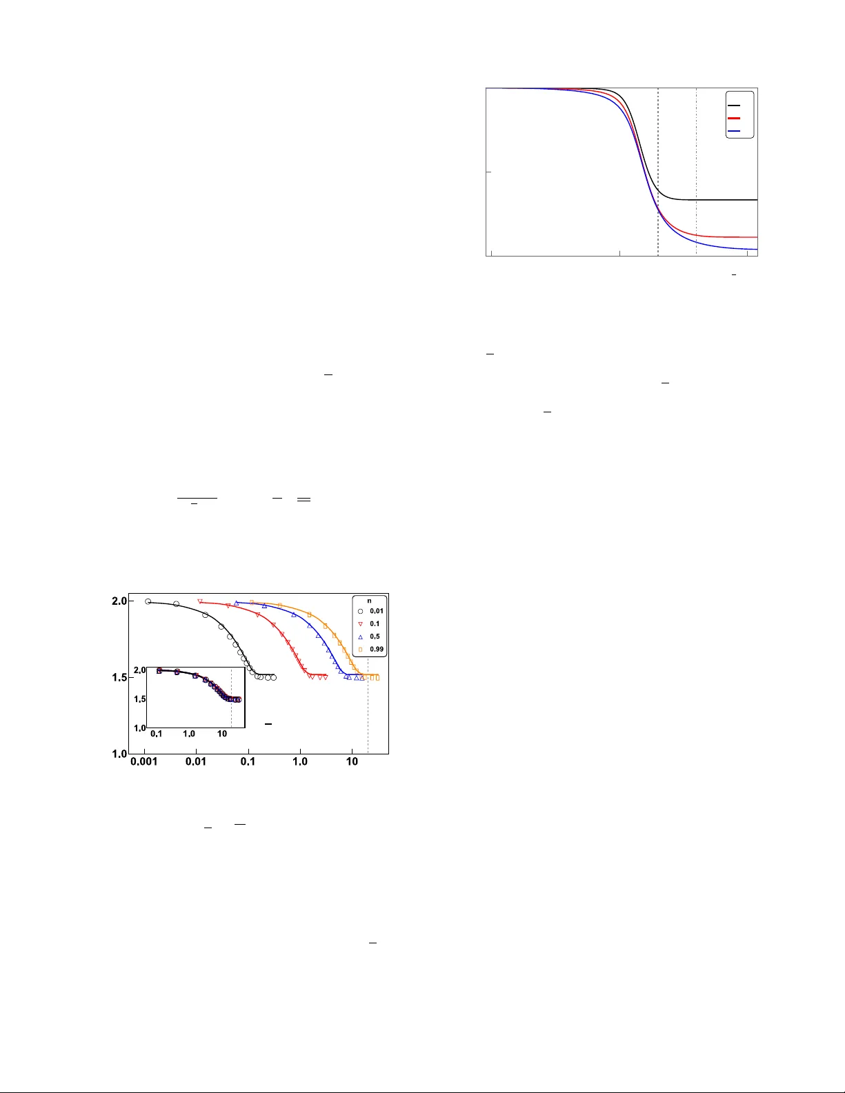
Thermo dynamics of statistical inference b y cells Alex H. Lang, 1 Charles K. Fisher, 1 Thierry Mora, 2 and Pank a j Mehta 1 1 Physics Dep artment, Boston University, Boston, Massachusetts 02215, USA 2 L ab or atoir e de physique statistique, CNRS, UPMC and ´ Ec ole normale sup´ erieur e, 75005 Paris, F r anc e The deep connection b et w een thermo dynamics, computation, and information is no w well estab- lished b oth theoretically and exp erimentally . Here, we extend these ideas to show that thermo- dynamics also places fundamental constraints on statistical estimation and learning. T o do so, w e in vestigate the constrain ts placed b y (nonequilibrium) thermodynamics on the abilit y of biochemical signaling netw orks to estimate the concen tration of an external signal. W e sho w that accuracy is limited by energy consumption, suggesting that there are fundamen tal thermo dynamic constraints on statistical inference. Cells often p erform complex computations in resp onse to external signals. These computations are implemen ted using elab orate bio c hemical netw orks that may op erate out of equilibrium and consume energy [1–7]. Given that energetic costs place imp ortant constrain ts on the design of ph ysical computing devices [8] and neural comput- ing architectures [9], one may conjecture that thermo- dynamic constraints also influence the design of cellular information pro cessing netw orks. This raises in tere sting questions ab out the relationship b etw een the informa- tion pro cessing capabilities of biochemical net works and energy consumption [10–14]. Indeed, we will sho w that thermo dynamics places fundamental constraints on the abilit y of bio chemical net works to perform statistical in- ference. More generally , statistical inference is intimately tied to the manipulation of information and hence offers a rich setting to study the relationship b et ween informa- tion and thermo dynamics [15–19]. In order for a cell to formulate an appropriate re- sp onse to an environmen tal signal, it m ust first estimate the concentration of an external signaling molecule us- ing membrane b ound receptors [1–6, 20]. The biophysics and biochemistry of cellular receptors is highly v ariable. Whereas some simple receptor proteins behav e lik e tw o- state systems (i.e. unbound and ligand bound) with dy- namics ob eying detailed balance [21], other receptors, suc h as G-protein coupled receptors (GPCRs), can ac- tiv ely consume energy as they cycle through multiple states. This naturally raises questions ab out ho w en- ergy consumption b y cellular receptors affects their abil- it y to perform statistical inference. Here, w e address these questions by analyzing the accuracy of statistical inference (i.e. learning) as a function of energy consump- tion in a simple but biophysically realistic mo del. W e sho w that learning more accurately alwa ys requires ex- p ending more energy , suggesting that the accuracy of a statistical estimator is fundamentally constrained by thermo dynamics. Cells estimate the concen tration of an external ligand using ligand-sp ecific receptors expressed on the cell sur- face. A ligand (usually a small molecule), at a con- cen tration c in the environmen t, binds the receptor at a concentration-dependent rate, k + c , and unbinds at a concen tration-indep enden t rate, k − [1] (see Fig. 1A). Up on ligand binding, the receptor protein undergo es con- formational changes or chemical mo difications that alter its activity , sending a signal that the ligand is b ound to do wnstream p ortions of the bio c hemical netw ork. Dur- ing a time in terv al T , the receptor can undergo multiple sto c hastic transitions b etw een the unbound nonsignaling state and the b ound signaling states. This information is con tained in the time series of signaling and nonsignaling in terv als (see Fig. 1B). After a time T , the cell con v erts this time series into an estimate for the external con- cen tration. A longer time series T alw ays giv es a b etter estimate for the concen tration; how ev er the cell needs to mak e a decision in a finite time, so w e consider T to be E. F. G. ADP ADP AT P AT P signal signal signal 0 0 1 2 1 k 10 k 10 k 01 k 01 k 21 k 12 k 02 k 20 signal signal signal 0 1 2 L k 10 k 01 k 21 k 12 k 0L k L0 A. k + c k - time Signaling Non- signaling T B. C. D. 𝞃 S 𝞃 NS FIG. 1: Schematic of a cell receptor and our mo del of a re- ceptor. (A) A c hemical ligand at concentration c binds to the receptor at rate k + c and unbinds at rate k − . (B) Ex- ample time series of a receptor binding. While unbound, the receptor is in nonsignaling state, but upon ligand binding it transitions to a signaling state. After a long time T , the recep- tor has a series of nonsignaling times τ N S and signaling times τ S from whic h to estimate the concen tration. (C) Two-state and (D) three-state bio c hemical models of a receptor. Up on ligand binding the receptor undergo es a ph ysical change (rep- resen ted as a conformational c hange) that transmits signals to the downstream bio c hemical net work. (E) Tw o-state, (F) three-state, and (G) L -state Mark ov mo dels of a receptor, where the c hain of states 3, 4, . . . L − 1 has b een suppressed. 2 fixed to a large but finite v alue. In principle, the esti- mate for the concen tration could b e computed using one of many different statistics that can b e obtained from this time series (e.g. a verage b ound time, av erage un- b ound time, etc.). Each of the resulting estimators for the external ligand concentration has a different accu- racy . F ollo wing Berg and Purcell (BP) [1], we measure the accuracy of an estimator for the concen tration using its “uncertain ty ,” defined as: uncertain ty := h ( δ c ) 2 i c 2 (1) where c is the mean and h ( δ c ) 2 i is the v ariance of the estimated concen tration. Sev eral methods ha ve b een proposed for how a cell ma y estimate the concentration of the external signaling molecule. In their pioneering pap er, Berg and Purcell suggested estimating the concen tration using the a verage time the receptor w as bound during the time T [1]. They sho wed that the minimal uncertain ty a receptor could ac hieve with this estimator was h ( δ c ) 2 i c 2 = 2 N (2) where N is the exp ected num b er of binding ev ents during the time interv al T . F or 30 y ears, man y thought that the BP estimator placed a fundamen tal limit on the accu- racy of a cellular receptor. How ever, in 2009, Endres and Wingreen [3] show ed that a cell using maxim um likeli- ho od estimation (MLE) based on the av erage nonsignal- ing time could reduce its uncertaint y b y half to h ( δ c ) 2 i c 2 = 1 N . (3) Ho wev er, the increased accuracy of MLE comes at an en- ergetic cost. Previous w ork [5] established that BP sets a limit for the b est p ossible estimator in equilibrium, im- plying that any receptor that performs MLE must op er- ate out of equilibrium and consume energy . In order to study the relationship b et ween thermody- namics and the accuracy of statistical estimators, we in- tro duce a new family of biophysically inspired cellular receptors that interpolate b et ween BP and MLE. In our mo del, receptors can activ ely consume energy by op erat- ing out of equilibrium (for example by hydrolyzing adeno- sine triphosphate or A TP). Using this family of models, w e show that there is a direct connection b et w een the energy consumed by a receptor and the uncertaint y of the resulting estimator. W e find that in order to learn more information (decrease its uncertaint y), the receptor m ust alwa ys exp end more energy (increase en tropy pro- duction). Note that, in this pap er, we restrict ourselves to mo deling the receptor and ignore the downstream sig- naling net w ork that con verts the signal from the receptor in to a cellular resp onse [10, 13]. Th us, the energies com- puted here represent low er b ounds on the total energy consumed b y the statistical estimation netw ork. Fig. 1C sho ws the simple tw o-state receptor considered b y BP . The binding of an external ligand to the receptor induces a change in the receptor from a nonsignaling state to a signaling state (see Fig 1B). The dynamics of this simple t wo-state receptor alwa ys obey detailed balance. Th us, in order to m odel nonequilibrium receptors, we m ust consider receptors with more than t w o states. Fig 1D sho ws a receptor with three states: one nonsignaling state to which ligands can bind, and t wo signaling states to which ligands cannot bind. With this extra state, the dynamics of the receptor can break detailed balance b y coupling the conformational change in the receptor to another reaction such as the hydrolosis of A TP . In particular, by consuming energy it is p ossible to drive the system preferentially through a series of state changes [22], for example clo c kwise in Fig 1F and Fig 1G. This results in a nonzero probabilit y flux through the state space and p ositive entrop y pro duction. In order to relate the thermodynamic properties of these receptors to their abilit y to p erform statistical in- ferences, it is useful to represent receptors as Marko v c hains. F or example, the tw o-state receptor shown in Fig. 1C can b e represented as a t wo-state Mark ov c hain with a state 0 corresp onding to the un bound nonsignal- ing state and state 1 corresp onding to the signaling state (see Fig. 1E). W e choose the transition rates b etw een states in the Mark ov chain to b e identical to the tran- sition rates b etw een conformations of the receptor. The three-state receptor can also b e mo deled as a three-state Mark ov chain with a ring structure, with state 0 once again corresp onding to the unbound, nonsignaling state (Fig. 1F). In this more abstract notation, it is easy to generalize the three-state receptor considered abov e to a receptor with L + 1 states (see Fig. 1G): L of these states are signaling states that cannot bind the ligand, while the remaining state, 0, corresp onds to the nonsignaling state that can bind ligands. F or ease of analysis, in this pap er, w e consider receptors arranged in a ring only . How ever, our mo del is a go od approximation for more complicated receptors with m ultiple path wa ys, so long as the receptor has a single path (for example, of length L ∗ ) that dom- inates the probability flux, see [23] for details. In that case, the complicated receptor reduces to a single ring of length L ∗ . A straightforw ard calculation shows that for the arc hi- tectures in Fig 1 [24], the uncertain ty of an estimate for the concen tration is given by [3]: h ( δ c ) 2 i c 2 = 1 N  1 + h ( δ τ S ) 2 i τ 2 S  ≡ E N (4) where N is the num b er of binding even ts, τ S is the mean time spent in the signaling state after binding a ligand, 3 and h ( δτ S ) 2 i is the v ariance of the time sp ent in the sig- naling states. In the second equality , we ha ve defined the co efficien t E which measures the accuracy of an estima- tor; e.g. E = 2 for the Berg-Purcell limit and E = 1 for MLE. F or a given estimator (i.e. a specific arc hitecture and a set of rates ~ k ), we can calculate the mean and the v ariance of the signaling time by a first passage calcula- tion similar to that in [24, 25]. Here w e pro vide some in tuition for Eq. (4). Notice that all the information about the ligand concentration is contained in the even t of a ligand binding to the re- ceptor, and the un binding of the ligand, or the exiting of the signaling state, is indep endent of concentration. Th us, any v ariation in the duration of the signaling state adds additional noise to the estimate but do es not contain an y more information ab out the concentration. There- fore, the optimal estimator is one where the signaling in terv als are completely deterministic and h ( δ τ S ) 2 i = 0. Comparing Eqs. (4) and (3), we see that this corresponds to MLE. This is consistent with the well-kno wn fact that MLE is the optimal unbiased estimator for large sam- ple sizes. When the durations of the signaling times are exp onen tially distributed, like for a tw o-state receptor, h ( δ τ S ) 2 i = τ 2 S , then Eq. (4) reduces to the BP re- sult given in Eq. (2). Finally , in all cases, the uncer- tain ty scales in versely with the a verage n umber of bind- ing ev en ts N during the time interv al T . This scaling la w follo ws from the central limit theorem by treating each binding even t as an indep endent sample of the concen- tration. The Mark o v represen tation allo ws us to calculate the energy consumption using ideas from nonequilibrium sta- tistical ph ysics. W e focus on long time interv als, T  1, with man y binding ev ents, where the receptor dynamics can be mo deled b y nonequilibrium steady states (NESS). The en tropy pro duction of the Mark o v pro cess is the energy p er unit time (p o wer) required to main tain this NESS, and therefore calculating the en trop y pro duction is equiv alen t to calculating the energy consumed by the bio c hemical net work[10, 22]. The en trop y production is giv en b y [26] e p = L X i =0 L X j 6 = i p ss i k ij ln k ij k j i , (5) with p ss i is the steady state probability of state i , k ij is the transition rate from state i to state j , and we hav e set k B T = 1 [24]. F or the architectures where the Marko v pro cess forms a ring, the entrop y pro duction simplifies to e p = ( p ss 0 k 01 − p ss 1 k 10 ) ln k 01 k 12 ...k L 0 k 0 L k 10 ...k L,L − 1 = J ln γ (6) where J is the net flux around the ring and ln γ is the free energy p er cycle [22, 24]. F or later reference, the total energy released in A TP hydrolysis is approximately 20 k B T at ro om temp erature[27]. W e note that previ- ous work inv estigating trade-offs b et w een accuracy and energy in Mark ov chains used a non-thermodynamically feasible energy [28]. Our goal is to find the b est p erforming estimator for a giv en receptor arc hitecture and en tropy pro duction (en- ergy consumption) rate. Ho wev er, there are sev eral bio- logical constrain ts that need to b e considered when op- timizing ov er c hoices of kinetic parameters. First, the rate at which a chemical ligand binds to a receptor is set by diffusion limited binding [1] and hence k 01 is not con trolled b y the cell. Therefore w e set k 01 = 1 and do not optimize ov er this rate. Second, a receptor needs to b e specific. In principle, b oth “correct” ligands (i.e. the ligands the receptor has ev olved to detect) and “wrong” ligands (an y other c hemical) can bind the receptor. How- ev er, nonsp ecific ligands quickly unbind and cause the receptor to switch back to the nonsignaling state. Thus, the specificity of a receptor is set b y the mean duration of the signaling state in the presence of the correct ligand, τ S . This is incorp orated by requiring a small nonsp ecific binding rate ( k 0 L =   1 = k 01 ) and we do not opti- mize o ver k 0 L . Lastly , since any statistical estimator is alw ays improv ed with more samples, to fairly compare differen t families of estimates, we will fix the sampling rate, n = N /T , where N is the exp ected num b er of sam- ples and T is the signal in tegration time. By fixing the nonsp ecific binding rate ( k 0 L ) to b e small [24], this im- plies τ S ≈ n − 1 − 1. But since we are also fixing the sampling rate, n , this fixes τ S . In summary , our goal is to find the global minima for uncertaint y , giv en the abov e constrain ts. W e b egin b y analyzing the three-state receptor (Fig. 1F). Figure 2 sho ws the uncertain ty as a function of en tropy production for the optimal threeistate recep- tor for four different c hoices of the ligand binding rate, ¯ n = N /T . T o generate these plots, w e hav e used an analytic ansatz[24] for the optimal parameters which w e ha ve chec ked using sim ulated annealing (with agreement within 1 . 25%). Notice that learning more accurately (re- ducing uncertaint y) alw a ys increased energy consump- tion (entrop y pro duction). A t low energy consump- tion, the receptor approaches the equilibrium BP limit ( E = 2), while at high energy consumption (corresp ond- ing approximately to the energy of A TP hydrolysis) the optimal p erformance asymptotically approaches the infi- nite en trop y production analytic limit of h ( δ c ) 2 i c 2 ∼ 3 2 N (7) One striking observ ation is that these curv es exhibit a data collapse when plotted as a function of the energy consumption p er ligand binding rate, e p /n . The inset of Fig. 2 shows the same curves as the main graph as a function of e p /n . Since eac h ligand binding even t can b e viewed as an indep enden t sample of the external con- 4 cen tration, this data collapse suggests that the natural v ariable linking thermo dynamics and inference is the en- ergy p er indep enden t sample consumed in constructing an estimator. The three-state receptor is not able to reac h the MLE limit of E = 1 for any level of entrop y pro duction. T o reac h the MLE limit, w e consider a receptor with L + 1 states, L of which are signaling states (see Fig. 1G). This Marko v chain has 2 L indep endent parameters, whic h makes it hard to find the global optimum. F or this reason, we analyzed a simplified, but still biophys- ically realistic, rate structure (without p erforming any optimization ov er parameters) where k 01 , k 0 L , k 10 , k L 0 can indep enden tly v ary but all other forward rates are fixed to b e iden tical, k i,i +1 = f and all other bac kw ard rates chosen so that k i +1 ,i = b , where i = 1 . . . L − 1 [24]. Once again, for all choices of L , the optimal uncer- tain ty exhibits a data collapse as a function of the energy consumption p er ligand binding rate, e p / n (see Fig. 3). A t low energy consumption, the uncertaint y approaches the BP limit ( E = 2), while at high energy consumption (corresp onding appro ximately to the energy of A TP hy- drolysis) asymptotically approac hes the infinite entrop y pro duction analytic limit of h ( δ c ) 2 i c 2 ∼  1 + 1 L  1 N (8) Th us, receptors with large energy consumption and man y signaling states ( L  1) approac h the MLE limit. In or- Entropy Production (e p ) Estimator ( E ) e p / n 1 A TP 1 A TP FIG. 2: Tw o signaling state estimator p erformance. F or v arying sampling rate n = N /T , the plot shows estimator p erformance ( E ) versus entrop y production ( e p with units of k B T = 1). The sym b ols represent results from simulated an- nealing, where k 01 = 1 and k 02 =  = 10 − 3 while the other four rates are optimized. The con tinuous lines represen t our ansatz[24] for the global minima. At high en tropy production the estimators asymptotically approach 1 . 5. The inset shows the data collapse when the estimator p erformance ( E ) is plot- ted versus entrop y production p er sampling rate ( e p / n ). The v ertical dashed line corresp onds to the approximate energy released by h ydrolysis of a single A TP . 1.0 10 100 1.0 1.5 2.0 1 A TP 2 A TP L 3 9 27 Entropy Production / Sampling Rate ( e p / n ) Estimator ( E ) FIG. 3: Illustrative example of L signaling state estimator p erformance. F or a v arying n um b er of signaling states L , the plot sho ws estimator p erformance ( E ) v ersus energy consump- tion ( e p /n ). F or an increasing L , at high energy consumption the estimator approaches the maximum lik elihoo d limit of 1. The following parameters are fixed at n = 0 . 99, k 01 = 1, k 0 L = 10 − 3 , α = k 10 /b = 10 − 3 , and ω = k L 0 /f = 1, while b w as v aried to keep n fixed, and θ = f /b was v aried to c hange the estimator and the energy consumption. These parame- ters were c hosen for conv enience and are not global optima. The vertical lines correspond to the appro ximate energy re- leased b y hydrolysis of a single A TP (dashes) or tw o A TPs (dot dashes). der to p erfectly achiev e the MLE limit, all backw ard rates b would need to b e 0, leading to infinite entrop y pro duc- tion. An interesting feature of these curv es is that b e- y ond some scale (whic h can be ac hiev ed b y h ydrolysis of only a few A TP), the marginal gain in improv ement that results from consuming more energy b ecomes negligible. This is reminiscent of the recently found transition in ki- netic pro ofreading where adding additional energy only marginally improv es the error threshold [23, 29]. It will b e interesting to see if this is a generic feature of many bio c hemical information pro cessing circuits. In conclusion, b y analyzing the ability of cells to es- timate the concentration of an external c hemical signal using nonequilibrium receptors we hav e established an unexp ected link b et ween statistical inference and ther- mo dynamics. Sp ecifically , w e found that the efficacy of an estimator for the concen tration of a ligand dep ends on the energy consumed p er indep enden t sample by the receptor. Extrapolating this result suggests that there ma y b e fundamen tal thermo dynamic b ounds on statisti- cal inference. The trade-off betw een accuracy and energy is general and may b e relev ant for other signal transduc- tion systems, such as gene regulation [30], ligh t-activ ated proteins [31] or ligand-gated ion channels [32]. W e note that follo wing the tradition of Berg and Purcell, in this pap er w e only considered estimating a concen tration af- ter a long time T . How ever, in man y related cases, suc h as transcription [33], the sp eed is an imp ortant trade- 5 off in addition to accuracy and energy consumption. In the con text of phosphorelays, it is likely that the circuits can resp ond quic kly even for m ultistep cascades. F or example, the four-stage phosphorelay utilized for pho- totransduction in the retina can still respond to stim uli in ab out half a second [34]. Nonetheless, understanding these trade-offs represents an imp ortan t future research direction. W e conjecture that our observ ed scaling, ( e p /n ), re- flects a general principle: the efficiency of a statistical estimator is limited b y the energy consumed per sample during its construction. Of course, muc h more inv esti- gation is needed to see if this conjecture holds in gen- eral. In particular, it will b e interesting to see if these results change for receptors mo deled b y heterogeneous Mark ov netw orks that are not strictly ringlik e in nature. Recen t work indicates that at large en tropy production the dynamics of suc h netw orks may b e indep endent of de- tails of the underlying top ology , suggesting that our basic picture should hold ev en for more complicated nonequi- librium receptors [35]. An additional extension to our mo del would b e to consider externally v arying concentra- tions b y implementing a sensory adaptiv e system (SAS) as was done in recen t pap ers[36, 37]. These pap ers found that the accuracy and energy consumption of the SAS dep ends on the time scale of external concentration fluc- tuations. Finally , it is well known that many receptors, suc h as GPCRs, actively consume energy in order to op- erate. Our mo del presents one possible explanation for this observ ation. The energy consumption ma y help re- duce noise in the downstream signal, allowing cells to more accurately determine external concentrations. Our mo del also shows that h ydrolysis of only one or tw o A TP nearly ac hieves the theoretical minima of uncertain t y . This ma y explain why cell sensors often require only a few phosphorylation sites. W e w ould lik e to thank David Sch wab and Ja v ad No or- bakhsh for the useful discussions. W e also thank Luca D’Alessio and DJ Strouse for detailed commen ts on the pap er. AHL w as supported by a National Science F oun- dation Graduate Research F ellowship (NSF GRFP) un- der Gran t No. DGE-1247312. PM and CKF were sup- p orted b y a Sloan Research F ello wship and a NIH K25 GM086909. [1] H. Berg and E. Purcell, Bioph ys. J. 20 , 193 (1977). [2] W. Bialek and S. Setay eshgar, Pro c. Natl. Acad. Sci. U.S.A. 102 , 10040 (2005). [3] R. Endres and N. Wingreen, Phys. Rev. Lett. 103 , 158101 (2009). [4] B. Hu, W. Chen, W. Rapp el, and H. Levine, Phys. Rev. Lett. 105 , 48104 (2010). [5] T. Mora and N. Wingreen, Ph ys. Rev. Lett. 104 , 248101 (2010). [6] V. Sourjik and N. S. Wingreen, Curr. Opin. Cell Bio. 24 , 262 (2012). [7] K. Kaizu, W. de Ronde, J. P aijmans, K. T ak ahashi, F. T ostevin, and P . R. ten W olde, Biophys. J. 106 , 976 (2014). [8] R. Landauer, IBM J. Res. Dev. 5 , 183 (1961). [9] S. Laughlin, Curr. Opin. Neurobiol. 11 , 475 (2001). [10] P . Meh ta and D. J. Sch wab, Proc. Natl. Acad. Sci. U.S.A. 109 , 17978 (2012). [11] G. Lan, P . Sartori, S. Neumann, V. Sourjik, and Y. T u, Nat. Phys. 8 , 422 (2012). [12] C. C. Gov ern and P . R. ten W olde, Phys. Rev. Lett. 109 , 218103 (2012). [13] C. C. Gov ern and P . R. ten W olde, (2013). [14] A. Barato, D. Hartich, and U. Seifert, Ph ys. Rev. E 87 , 042104 (2013). [15] A. Berut, A. Arakely an, A. Petrosy an, S. Cilib erto, R. Dillensc hneider, and E. Lutz, Nature 483 , 187 (2012). [16] D. Mandal and C. Jarzynski, Pro c. Natl. Acad. Sci. U.S.A. 109 , 11641 (2012). [17] S. V aikuntanathan and C. Jarzynski, Phys. Rev. E 83 , 061120 (2011). [18] T. Saga wa and M. Ueda, Phys. Rev. E 85 , 021104 (2012). [19] S. Still, D. A. Siv ak, A. J. Bell, and G. E. Cro oks, Ph ys. Rev. Lett. 109 , 120604 (2012). [20] X. Cheng, L. Merc han, M. Tchernooko v, and I. Nemen- man, Phys. Bio. 10 , 035008 (2013). [21] J. E. Keymer, R. G. Endres, M. Skoge, Y. Meir, and N. S. Wingreen, Proc. Natl. Acad. Sci. U.S.A. 103 , 1786 (2006). [22] T.L. Hill, F r e e ener gy tr ansduction and bio chemical cycle kinetics , (Springer, 1989). [23] A. Murugan, D. A. Huse, and S. Leibler, Pro c. Natl. Acad. Sci. U.S.A. 109 , 12034 (2012). [24] See Supplementary Material for additional details. [25] G. Bel, B. Munsky , and I. Nemenman, Phys. Bio. 7 , 016003 (2010). [26] J. Leb owitz and H. Sp ohn, J. Stat. Phys. 95 , 333 (1999). [27] D. V o et and J. V o et, Bio chemistry (John Wiley and Sons New Y ork, 2004), 3rd ed. (pg 566, T able 16.3) [28] S. Escola, M. Eisele, K. Miller, and L. Paninski, Neural computation 21 , 1863 (2009). [29] B. Munsky , I. Nemenman, and G. Bel, The J. Chem. Ph ys 131 , (2009). [30] D. M. Suter, N. Molina, D. Gatfield, K. Schneider, U. Schibler, and F. Naef, Science 332 , 472 (2011). [31] W. Bialek, Biophysics: Se ar ching for Principles (Prince- ton Universit y Press, 2012). [32] L. Csan´ ady , P . V ergani, and D. C. Gadsby , Proc. Natl. Acad. Sci. U.S.A. 107 , 1241 (2010). [33] M. Depken, J. M. Parrondo, and S. W. Grill, Cell Rep orts 5 , 521 (2013). [34] P . B. Detwiler, S. Ramanathan, A. Sengupta, and B. I. Shraiman, Biophysical Journal 79 , 2801 (2000). [35] S. V aikuntanathan, T. R. Gingric h, and P . L. Geissler, Ph ys. Rev. E 89 , 062108 (2014). [36] P . Sartori, L. Granger, C. F. Lee, and J. M. Horowitz, arXiv:1404.1027 (2014). [37] A. C. Barato, D. Hartich, and U. Seifert, (2014). [38] S. Redner, A Guide to First-Passage Pr o c esses (Cam- bridge, 2001). [39] R. A. Blythe, Master’s thesis, Edin burgh (2001). 6 [40] F. Hussain, C. Gupta, A. J. Hirning, W. Ott, K. S. Matthews, K. Josi ´ c, and M. R. Bennett, Pro ceedings of the National Academy of Sciences 111 , 972 (2014). [41] I. H. Segel, Enzyme Kinetics , vol. 360 (Wiley , New Y ork, 1975). Supplemen tary Material Notation Here we pro vide more details of the results in the main text. First, w e outline our notation. The time dependent probabilit y of state i is p i = p i ( t ), while the steady state probability of state i is p ss i . The Laplace transformed probabilit y of state i is P i ( s ). The rate to go from state i to state j is k ij . The probability to transition from state i to state j is q ij . The time it tak es to transition from state i to j is τ ij . The first passage time is given b y f ( t ) while the Laplace transformed first passage time is F ( s ). The lifetime of state i is ρ i . Detailed Deriv ation of General Uncertain t y Here w e deriv e form ulas for the accuracy of statistical inference when the activ ated signaling states contin uously pro duce signals. F ollowing Berg and Purcell [1], w e will measure the accuracy of a receptor by the “uncertain t y” of the concen tration estimate: uncertain ty := h ( δ c ) 2 i c 2 (9) where c is the mean and h ( δ c ) 2 i is the v ariance of the estimated concen tration. Let us consider the case where activ ated signaling states pro duce do wnstream signaling molecules at a rate α . W e will define τ S as the mean lifetime of the signaling states and τ N S as the mean non-signaling time. Then, we kno w that the mean n umber of signaling molecules u pro duced after a time T is given by u = αT  τ S τ S + τ N S  ≡ αT ¯ φ (10) This follows b y noting that ¯ φ is just the fraction of time the receptor is in the signaling states. Notice that by definition, α and T are indep endent of the concen tration c . The signaling time τ S , can in principle dep end on concen tration, and for L signaling states is giv en b y τ S = L X i =1 p 0 i τ i 0 (11) where p 0 i is the probabilit y to transition from state 0 to state i , and τ i 0 is the mean time to return from state i to state 0. Since w e assume the receiving state is strongly biased (i.e. k 01 is muc h larger than any other rate k 0 i from non-signaling, 0, to signaling state i ), then the deriv ativ e of the signaling time with resp ect to concentration is: dτ S dc = − L X i =2 k 0 i k 01 ( τ 10 + τ i 0 ) (12) Since this is b y assumption small, we will approximate τ S as independent of concen tration, and thus all the concen- tration dependence comes from τ N S . Thus, using the usual error-propagation formulas one has δ u u = − dτ N S dc 1 τ S + τ N S δ c (13) whic h giv es the uncertaint y for the concen tration: h ( δ c ) 2 i c 2 =  c dτ N S dc  − 2 ( τ N S + τ S ) 2 h ( δ u ) 2 i u 2 (14) 7 The formula ab o ve reduces the problem to calculating the uncertaint y in the num b er of signaling molecules pro duced in a time T . T o calculate this, notice that u comes from on av erage N = T / ( τ S + τ N S ) indep enden t binding cycles (state 0 to state 1 transition). Th us, the v ariance in the fraction of time bound during a time T will just b e N − 1 times the v ariance in a single binding cycle. In particular, the co efficien t of v ariation in a single cycle is giv en b y δ φ φ = τ N S τ S + τ N S  δ τ S τ S  −  δ τ N S τ N S  (15) Noting that the signaling and non-signaling ev ents are independent, w e get h ( δ u ) 2 i u 2 = 1 N  τ N S τ S + τ N S  2  h ( δ τ N S ) 2 i τ 2 N S + h ( δ τ S ) 2 i τ 2 S  (16) Plugging this expressions in to (14) gives h ( δ c ) 2 i c 2 = 1 N  c d log ( τ N S ) dc  − 2  h ( δ τ N S ) 2 i τ 2 N S + h ( δ τ S ) 2 i τ 2 S  (17) Therefore the complicated resp onse of a receptor is reduced to its mean and v ariance of the time in b oth the signaling and non-signaling states. In this pap er, we will examine the case where there is a single non-signaling state (0) and there are L signaling states arranged in a ring. In this case, the ab ov e expression simplifies to (leading order k 0 L /k 01 ): h ( δ c ) 2 i c 2 = 1 N  1 + h ( δ τ S ) 2 i τ 2 S  (18) F or a tw o state pro cess as considered by Mora and Wingreen [5], there is only the receiving state and one signaling state. These are just P oisson processes which eac h ha ve an uncertaint y of 1 and w e recov er the Berg and Purcell [1] limit h ( δ c ) 2 i c 2 = 2 N (19) General First Passage Time W e need to calculate the first passage prop erties of the Marko v chain, specifically the mean and v ariance of the first passage time. This can b e calculated as follows [25, 38]. The master equation that w e wan t to solv e is dp dt = K p ( t ). First apply the Laplace transform P i ( s ) = Z ∞ 0 p i ( t ) e − st dt (20) whic h leads to the master equation ( s − K ) P ( s ) = p ( t = 0) (21) with K the matrix of transitions for the full system but with the transition rates lea ving the absorbing states set to zero. The first passage time to return to state 0 is f ( t ) = dp 0 ( t ) dt (22) F ( s ) = sP 0 ( s ) (23) F or our purp oses, w e only need the mean and v ariance of the first passage time. This is easily obtained by the uncen tered momen ts M ( m ) = Z ∞ 0 t m f ( t ) = ( − 1) m d m F ( s ) ds m     s =0 (24) 8 where m = 1 is the mean and m = 2 is the uncen tered second moment. In general w e kno w that τ x , the spent in state x , is dra wn from a mixture where it can switc h to states j = 1 , 2 , ... . The v ariance of mixtures is X = P i w i X i , where w i are arbitrary weigh ts and X i are random v ariables drawn from distributions with mean µ i and v ariance σ i . Combining equations we get: V ar(X) = X i w i  ( µ i − µ ) 2 + σ 2 i  (25) with µ = P i w i µ i . W e can get the time sp en t in state x , τ x , by using the v ariance mixture form ula combined with τ ix and V ar( τ ix ), resp ectiv ely the mean and v ariance first passage time of starting in state i and ending in state x . This giv es us τ x = X i q xi τ ix (26) q xi = k xi P j k xj = k xi ρ x (27) ρ x =   X j k xj   − 1 (28) V ar( τ x ) = X i q xi V ar ( τ ix ) + X i q xi τ ix − X k q xk τ kx ! 2 (29) where q xi is the probabilit y of transitioning from state x to state i , k xi is the rate to go from state x to state i , and ρ x is the lifetime of state x . In this pap er, w e hav e one non-signaling state and the other L states are signaling. Therefore, w e will let state 0 b e the absorbing state, and it can initially transition to state 1 and state L . The abov e equations then simplify to τ 0 = q 01 τ 10 + q 0 L τ L 0 (30) V ar( τ 0 ) = q 01 V ar ( τ 10 ) + q 0 L V ar ( τ L 0 ) + 2 q 01 q 0 L ( τ 10 − τ L 0 ) 2 (31) q 0 L = 1 − q 01 (32) First Passage Time: 2 Signaling States Here we calculate the mean and v ariance of the first passage time to return to state 0 from either state 1 or 2. The master equation that w e need to solve is dp dt = K p ( t ). The matrix rates are: K ij =                        k 10 for i = 0 and j = 1 k 12 for i = 2 and j = 1 k 20 for i = 0 and j = 2 k 21 for i = 1 and j = 2 − ( k 10 + k 12 ) for i = 1 and j = 1 − ( k 20 + k 21 ) for i = 2 and j = 2 0 ev erywhere else (33) While the initial conditions are set by the rates k 01 and k 02 , for the purp oses of the first passage time calculation, the rates from 0 to 1 ( k 01 ) and from 0 to 2 ( k 02 ) are b oth set to zero, k 01 = k 02 = 0. The Laplace transform for the initial condition of starting in state 1 is: F ( s ) = sP 0 ( s ) = k 10 P 1 + k 20 P 2 (34) 9 with P 1 =  Γ 1 − k 12 k 21 Γ 2  − 1 (35) P 2 = k 12 Γ 2 P 1 (36) Γ i = s + ρ − 1 i (37) W e can obtain mean and v ariance from τ = − dF ds     s =0 (38) V ar( τ ) = d 2 F ds 2     s =0 − τ 2 (39) The mean and v ariance of the first passage time from starting in either state 1 or state 2 is: τ 10 = ρ 1 1 + k 12 ρ 2 1 − k 12 k 21 ρ 1 ρ 2 = k 12 + k 20 + k 21 ξ (40) τ 20 = ρ 2 1 + k 21 ρ 1 1 − k 12 k 21 ρ 1 ρ 2 = k 10 + k 12 + k 21 ξ (41) V ar( τ 10 ) = τ 2 10  1 + 2 ρ 2 2 k 12 ( k 10 − k 20 ) (1 + k 12 ρ 2 ) 2  = τ 2 10 + 2 k 12 ( k 10 − k 20 ) ξ 2 (42) V ar( τ 20 ) = τ 2 20  1 + 2 ρ 2 1 k 21 ( k 20 − k 10 ) (1 + k 21 ρ 1 ) 2  = τ 2 20 − 2 k 21 ( k 10 − k 20 ) ξ 2 (43) ξ = k 10 k 20 + k 10 k 21 + k 12 k 20 (44) where the second equalit y holds as long as ξ 6 = 0. First Passage Time: L Signaling States Deriv ation Here we calculate the mean and v ariance of the first passage time in a L + 1 state c hain. The master equation that w e need to solve is dp dt = K p ( t ). The matrix is indexed from 0 to L and the rates are: K ij =                              k 10 for i = 0 and j = 1 k L 0 for i = 0 and j = L f for i = j + 1 and 1 < j < L b for i = j − 1 and 1 < j < L − ( f + k 10 ) for i = 1 and j = 1 − ( f + b ) for i = j and 1 < j < L − ( k L 0 + b ) for i = L and j = L 0 ev erywhere else (45) While the initial conditions are set by the rates k 01 and k 0 L , for the purposes of the first passage time calculation, the rates from 0 to 1 ( k 01 ) and from 0 to L ( k 0 L ) are b oth set to zero, k 01 = k 0 L = 0. F or later con venience we define the follo wing ratio of rates: θ = f b (46) α = k 10 b (47) ω = k L 0 f (48) 10 W e can use a transfer matrix to find a general solution (for non-degenerate eigenv ales, i.e. θ 6 = 1) to the state probabilit y as P i ( s ) = C + λ i − 1 + + C − λ i − 1 − (49) Solving for the the expressions 1 < i < L leads to λ ± = 1 2 b  s + f + b ± p ( s + f + b ) 2 − 4 f b  (50) = 1 2  σ ± p σ 2 − 4 θ  = 1 2 ( σ ± ψ ) (51) σ = s b + θ + 1 (52) ψ = p σ 2 − 4 θ (53) With the initial condition of starting in P 1 , the b oundary equations for P 1 and P L are: ( σ + α − 1) ( C + + C − ) = 1 /b + ( C + λ + + C − λ − ) (54) ( σ + ( ω − 1) θ )  C + λ L − 1 + + C − λ L − 1 −  = θ  C + λ L − 2 + + C − λ L − 2 −  (55) Solving these equations giv es C − = − C + Λ L M (56) C + = 1 b [ λ − + α − 1 − ( λ + + α − 1)Λ L M ] (57) Λ = λ + λ − (58) M = 1 + ( ω − 1) λ − 1 + ( ω − 1) λ + (59) And then the probabilities are P 1 ( s ) = C +  1 − Λ L M  (60) P L ( s ) = C + λ L − 1 + (1 − Λ M ) (61) signal signal signal 0 1 2 L k 10 k 01 b f k 0L k L0 FIG. 4: Simplified rate structure considered for L signaling states first passage time calculation. The rates k 01 , k 10 , k L 0 , k 0 L are unconstrained, while the remaining forward rates are equal, f = k 12 = k 23 = . . . = k L − 1 ,L and the remaining bac kw ard rates are equal, b = k 21 = k 32 = . . . = k L,L − 1 . 11 The full Laplace transform F is: F ( s ) = α (1 − Λ L M ) + ω θ λ L − 1 + (1 − Λ M ) λ − + α − 1 − ( λ + + α − 1)Λ L M (62) Results T o get the mean and v ariance of the first passage time, we need τ 10 = − dF ds     s =0 (63) V ar( τ 10 ) = d 2 F ds 2     s =0 − τ 2 (64) The mean return time to state 0 when starting in state 1 is: τ 10 = τ 10 ,num τ 10 ,den (65) τ 10 ,num = ( ω L − ω + 1) θ L +1 − ( ω L + 1) θ L + ( ω − 1) θ + 1 (66) τ 10 ,den = b [ θ − 1]  ω θ L +1 + ω ( α − 1) θ L + α (1 − ω ) θ − α  (67) The v ariance of the return time to state 0 when starting in state 1 is: V ar( τ 10 ) = V ar( τ 10 ) num V ar( τ 10 ) den (68) V ar( τ 10 ) num = θ 2 L +3  ω 2 ( L − 1) + 1  (69) + θ 2 L +2  ω 2  L 2 α − L (3 α + 1) + 2 α − 3  + 2 ω (( L − 2) α + 1) + 2 α − 3  − θ 2 L +1  ω 2  2 L 2 α − 4 Lα + L + 4 α − 4  + ω ((4 L − 6) α + 4) + 4 α − 3  + θ 2 L [ ω ( ω L + 2)( Lα − α + 1) + 2 α − 1] + θ L +3 ( ω − 1)  2( ω − 1) α + 3 ω L 2 α + L ( ω (4 − 5 α ) + 4 α ) + 2  + θ L +2  − 2 ω 2  3 L 2 α + L (4 − 6 α ) + α − 2  + θ L +2  ω  9 L 2 α + L (12 − 23 α ) + 8 α − 6  + 6(2 L − 1) α + 6  + θ L +1  ω  − 9 L 2 α + L (19 α − 12) − 6 α + 6  + θ L +1  ω 2 ( L − 1)((3 L − 4) α + 4) + 6( − 2 Lα + α − 1)  + θ L  α  3 L 2 ω − 5 Lω + 4 L + 2 ω − 2  + (4 L − 2) ω + 2  − θ 3 ( ω − 1) 2 (2 α − 1) − θ 2 ( ω − 1)( ω + 4 α − 3) + θ ( − 2 ω − 2 α + 3) − 1 V ar( τ 10 ) den = b 2 [ θ − 1] 3  ω θ L +1 + ω ( α − 1) θ L + α (1 − ω ) θ − α  2 (70) While the results here are for initial condition of b eing in state 1, one can easily find the results for the initial condition of state L if one mak es the following substitutions θ ⇔ 1 /θ , b ⇔ f , and α ⇔ ω . Steady State Probabilities In general, we are considering a Marko v c hain with L + 1 nodes (lab eled 0 to L ). W e ha ve the master equation dP ( t ) dt = K P ( t ) (71) 12 with K the matrix of transition rates. The rates are lab eled as k ij where i is the initial state and j is the final state. F or later con venience, define the lifetime of a state as ρ i =   X j 6 = i k ij   − 1 (72) The steady state distributions are easily obtained by solving K p ss = 0. The solution can b e written in a compact form [39] as P ss i = z i Z (73) Z = X i z i (74) and z i is the matrix minor of K at ( i, i ) i.e. the determinan t of K with the i th row and column remov ed. F or the t wo signaling state system we ha ve that p ss 0 = ρ − 1 1 ρ − 1 2 − k 12 k 21 Z = k 10 k 20 + k 10 k 21 + k 12 k 20 Z (75) p ss 1 = ρ − 1 0 ρ − 1 2 − k 02 k 20 Z = k 01 k 20 + k 01 k 21 + k 02 k 21 Z (76) p ss 2 = ρ − 1 0 ρ − 1 1 − k 01 k 10 Z = k 01 k 12 + k 02 k 10 + k 02 k 12 Z (77) Z = X i 6 = j  ρ − 1 i ρ − 1 j − k ij k j i  (78) F or the L signaling state with the simplified rates, we will just presen t the result for state 0: p ss 0 = p ss 0 ,num p ss 0 ,den (79) p ss 0 ,num = b ( θ − 1)  ω θ L +1 + ω ( α − 1) θ L + α (1 − ω ) θ − α  (80) p ss 0 ,den = − α + αb + αL +  + 1 (81) + θ ( αbω − 2 αb − αL + ω −  − 1) (82) + αbθ 2 (1 − ω ) (83) + θ L ( bω + α − Lω − 1 −  − αbω ) (84) + θ 1+ L ( αbω − 2 bω + Lω − ω + 1 +  ) (85) + bω θ L +2 (86) The rates from 0 to 1 is k 01 = 1, from 1 to 0 is k 10 (with α = k 10 /b ), from 0 to L is k 0 L =   1, and from L to 0 is k L 0 (with ω = k L 0 /f ). All other forw ard rates are f and bac kward rates are b and the ratio of rates is θ = f /b . Av erage Sampling Rate: n The a v erage sampling rate is n = N T = k 01 p ss 0 (87) where N is the n umber of samples (i.e. num b er of binding even ts), T is the total in tegration time, k 01 is the rate from state 0 to state 1, and p ss 0 is the steady state probabilit y of being in state 0. Since we are assuming that k 01 = 1 and k L 0 =   1, we hav e the mean signaling time b ecomes τ S ≈ τ 10 . With these rates we hav e n ≈ (1 + τ S ) − 1 (88) 13 En tropy Production: e p F or a general Marko v process with states lab eled by i , steady state probabilities p ss i , and transition rate k ij from state i to state j , the non-equilibrium steady state (NESS) entrop y pro duction [10, 26] is given by e p = L X i =0 L X j 6 = i p ss i k ij ln k ij k j i (89) where the summation is o v er both i and j . Alternativ ely , the en tropy pro duction can b e written as a sum ov er the flux betw e en each connected no de as e p = L X i =0 L X j >i ( p ss i k ij − p ss i k ij ) ln k ij k j i (90) where no w we ha ve an unrestricted sum ov er i but a restricted sum ov er j . Since w e are mo deling our receptor as a ring, the en tropy production simplifies to e p = ( p ss 0 k 01 − p ss 1 k 10 ) ln k 01 k 12 . . . k L 0 k 0 L k 10 . . . k L,L − 1 = J ln γ (91) where the flux J = p ss 0 k 01 − p ss 1 k 10 b et w een each neigh b oring state is equal and the ln γ is the free energy difference of a cycle. F or 2 signaling states, the en tropy pro duction p er sampling rate is given by: e p n =  1 + k 10 k 12 + k 10 k 21 k 12 k 20  − 1 γ − 1 γ ln γ (92) γ = k 01 k 12 k 20 k 10 k 21 k 02 (93) F or the L signaling states arranged in a ring, the en tropy pro duction per sampling rate is giv en b y: e p n =  1 + α ω θ − L + α θ − 1 1 − θ 1 − L 1 − θ − 1  − 1 γ − 1 γ ln γ (94) γ = k 01 ω k 0 L α θ L (95) where ω = k L 0 /f , α = k 10 /b , θ = f /b , f is all the forw ard rates (except k 01 and k L 0 ), and b is all the bac kward rates (except k 10 and k 0 L ). Ansatz for 2 Signaling State Receptor Here are the details of the ansatz for the minim um uncertain ty for the 2 signaling state system. The rates are as follo ws: • k 01 = 1 • k 10 = k 2 (1 − x ) • k 12 = k x • k 21 = k δ • k 20 = k • k 02 =  14 where   1 (and in this pap er  = 10 − 3 ), 0 < x < 1, δ  1 (and in this paper δ = 0 . 04), and k is v aried to fix the mean sampling rate n . F or the ansatz, the mean, coefficient of v ariation, and entrop y production simplifies to τ S ≈ 2 k (96) h ( δ τ S ) 2 i τ 2 S ≈ 1 − x 1 + x (97) e p n ≈  1 + 1 − x 2 x  − 1 γ − 1 γ ln γ (98) γ = 2 x δ (1 − x ) (99) Sim ulated Annealing Sim ulated annealing is a meta-heuristic algorithm for global optimization in which one uses the Metrop olis algorithm to p erform a random walk in parameter space while p erio dically low ering the temp erature. W e used a simulated annealing algorithm to search for the parameters of a model describing a receptor with 2 signaling states that minimizes a cost function giv en b y cost = h ( δ c ) 2 i ¯ c 2 + λ e p (ln e p − ln ˆ e p ) 2 − ( λ n ˆ n − 1) ln n − ( λ n (1 − ˆ n ) − 1) ln(1 − n ) (100) That is, we minimize the uncertaint y of the resulting estimator ( h ( δ c ) 2 i / ¯ c 2 ) sub ject to soft constrain ts on the energy pro duction ( e p ) and sampling rate ( n ), which are constrained to ˆ e p and ˆ n , resp ectively . Here, λ e p and λ n implemen t the constrain ts. W e c hose λ e p = 20 and λ n = 20 / max { ˆ n, 1 − ˆ n } . Let Ω 1 denote a set of parameters describing a receptor with 2 signaling states (i.e. all of the v arious rate constan ts). A new set of trial parameters Ω 2 w as generated in the follo wing w ay: for eac h k ∈ Ω 1 set the corresponding k 0 ∈ Ω 2 to ln k 0 = ln k + η where η is a random v ariable with from a Normal distribution cen tered at zero. The width of the signal signal 0 1 2 k 10 k 10 = k(1-x)/2 1 k δ kx ε k FIG. 5: Rate structure for ansatz of minim um uncertain ty for the L = 2 signaling state system. The rates are as follo ws: k 01 = 1, k 10 = k 2 (1 − x ), k 12 = kx , k 21 = kδ , k 20 = k , and k 02 =  . The mean signaling time is set b y k . The other rates are , δ  1 and 0 < x < 1. 15 Normal distribution w as chosen adaptively so that approximately 25% of the steps were accepted. Making the random p erturbations to the logarithm of the rate constants ensures that they are alw ays p ositive. The trial mo v e was accepted according to the Metropolis criterion with probability min[1 , exp((cost(Ω 1 ) − cost(Ω 2 )) /T )]. The temperature T w as initialized to T = 10 and adjusted b y T ← 0 . 95 T every 2000 steps. The b est solution obtained during the chain was stored in Ω B , and the chain was re-initialized from Ω 1 = Ω B ev ery 2000 steps to preven t the chain from getting stuck in a p o or local minim um. This sim ulated annealing algorithm was run until conv ergence of h ( δ c ) 2 i / ¯ c 2 , e p and n . Scaling with T emp erature In the main text, we work ed in the units of k B T = 1. How ev er, here we examine the general temp erature dep endence. Exp erimen tally , it is known that rates of biochemical reactions doubles for ev ery 10 ◦ C [40, 41]. Therefore, a general rate k at a temp erature T (measured in degrees Celsius) is related to initial rate k 0 and initial temp erature T 0 b y: k = k 0 2 T − T 0 10 (101) No w we need to determine the general scaling of v arious entities in this pap er, which is summarized b elow in terms of a general rate k : • Mean signaling time, τ S ∼ k − 1 • V ariance in signaling time, h ( δ τ S ) 2 i ∼ k − 2 • Co efficien t of v ariation of signaling time, h ( δ τ S ) 2 i τ 2 S ∼ 1 • Sampling rate, n ∼ k • Uncertainity , h ( δ c ) 2 i c 2 ∼ k − 1 • Entrop y pro duction, e p ∼ k While increasing temp erature increases b oth the mean and v ariance of the signaling time, since the estimator ( E = 1 + h ( δ τ S ) 2 i τ 2 S ) only dep ends on the co efficien t of v ariation of signaling time, the estimator is indep enden t of temp erature. The sampling rate n does increase with increasing temperature, and therefore increasing temp erature decreases the uncertaint y . How ev er, this decrease in uncertaint y costs energy . While the free energy p er cycle (ln γ ) remains constant, the probability flux ( J ) is prop ortional to a rate, and since the entrop y pro duction is giv en by e p = J ln γ , w e see that that decrease in uncertaint y is directly related to the increase in en trop y production.