A Note on Archetypal Analysis and the Approximation of Convex Hulls

We briefly review the basic ideas behind archetypal analysis for matrix factorization and discuss its behavior in approximating the convex hull of a data sample. We then ask how good such approximations can be and consider different cases. Understanding archetypal analysis as the problem of computing a convexity constrained low-rank approximation of the identity matrix provides estimates for archetypal analysis and the SiVM heuristic.

💡 Research Summary

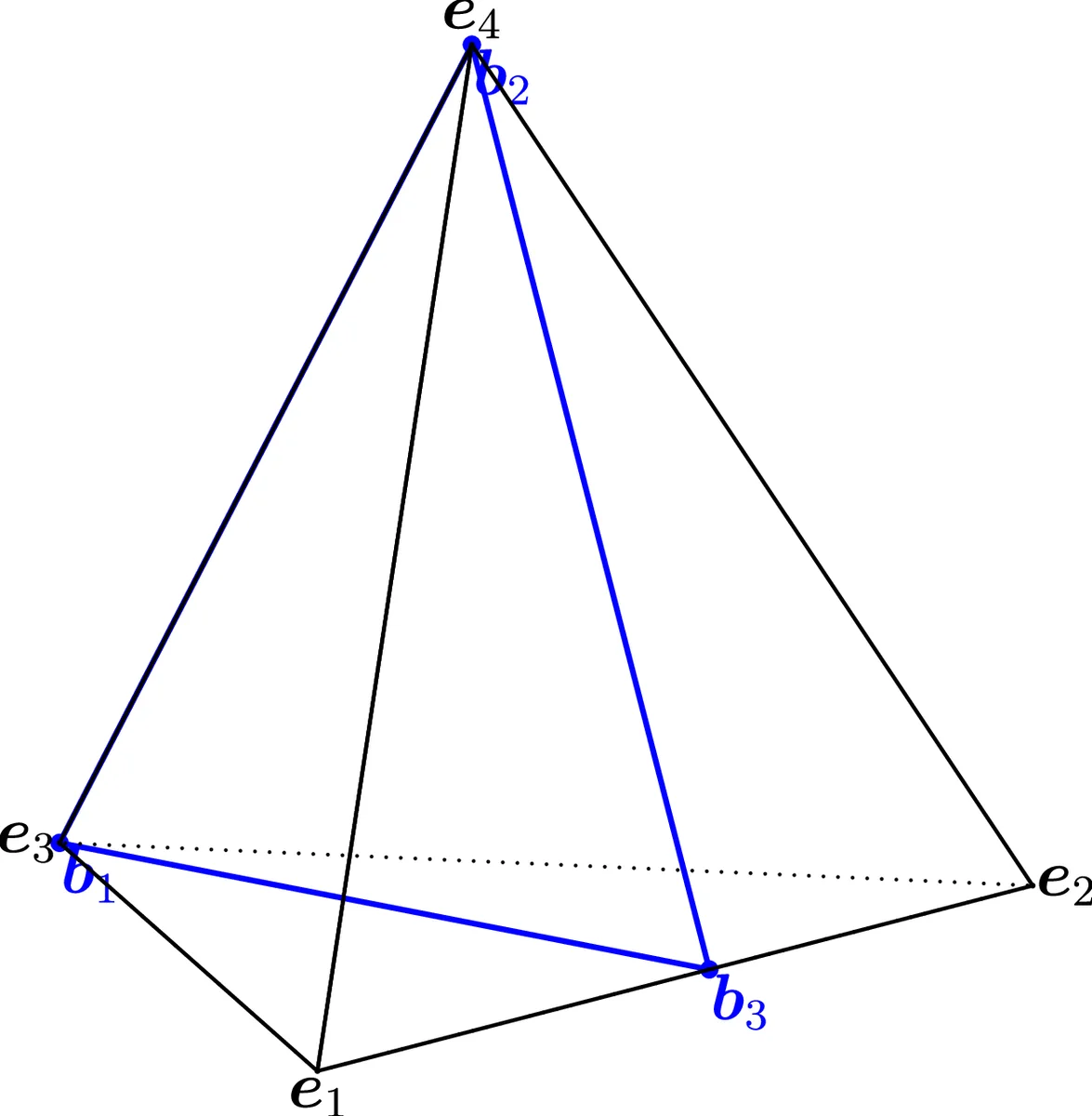
This paper revisits archetypal analysis (AA), a matrix factorization technique introduced by Cutler and Breiman, and examines its ability to approximate the convex hull of a data set. In AA one seeks two column‑stochastic matrices B (size n × k) and A (size k × n) such that X ≈ XBA = ZA, where Z = XB contains k “archetypes”. Each archetype is a convex combination of the original data points, and each data point is in turn approximated as a convex combination of the archetypes, giving the method an appealing symmetry and interpretability.

The authors first note that if the number of archetypes k equals the number of data points n, the identity matrix I can be used for both B and A, yielding a perfect reconstruction. More interestingly, perfect reconstruction is also possible when k equals the number q of vertices of the data convex hull: the vertices themselves become the unique global minimizers of the AA objective. This observation motivates a reduction of the original problem to a smaller one that only involves the vertex matrix V ∈ ℝ^{m×q}. The reduced problem is to minimize ‖V – VBA‖_F^2, which can be rewritten as ‖V(I – BA)‖_F^2. Because B and A are column‑stochastic, the product BA lies inside the standard simplex Δ^{q‑1}. Consequently, AA can be interpreted as a convexity‑constrained low‑rank approximation of the identity matrix I_q.

Two lemmas establish fundamental limits. Lemma 1 proves that when k < q a perfect low‑rank approximation of I_q is impossible, because each column of I_q is an extreme point of the simplex and cannot be expressed as a convex combination of fewer than q stochastic vectors. Lemma 2 provides a worst‑case upper bound: ‖I – BA‖_F^2 ≤ 2q. This follows from the fact that any two vertices of Δ^{q‑1} are at distance √2, so the squared Frobenius norm, which sums the squared distances of all q columns, cannot exceed 2q. Combining this with the reduction yields the bound ‖V(I – BA)‖_F^2 ≤ 2q‖V‖_F^2, showing that the number of extreme points q directly influences the potential error.

The paper then analyses the SiVM (Simplex Volume Maximization) heuristic, a greedy algorithm that selects k data points that are as far apart as possible and uses them as archetypes. Geometrically, SiVM places the k columns of B on k vertices of Δ^{q‑1}. The remaining q – k vertices are approximated by their orthogonal projection onto the (k‑1)-dimensional subsimplex spanned by the selected vertices. The distance d from any omitted vertex to this subsimplex equals the height of the simplex formed by the k chosen vertices plus the omitted one, which can be expressed as d = √