Confidence-based Optimization for the Newsvendor Problem

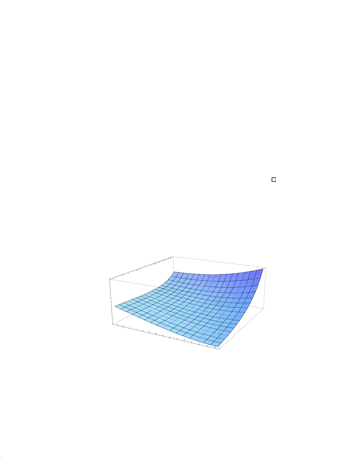
Conﬁdence-based Optimization for the Newsv endor Problem Rob erto Rossi Universit y of Edinburgh Business School, UK, roberto.rossi@ed.ac.uk Stev en Prest wic h Dept. of Computer Science, Universit y College Cork, I reland, s.prest wich@4c.ucc.i e S. Armagan T arim Dept. of Management, Hacettepe U niv ersity , T urkey , armagan.tarim@hacettepe.edu.tr Brahim Hnic h Dept. of Computer Engineering, Izmir Universit y of Economics, T urkey , brahim.hnich@ieu.edu.tr Abstract W e introduce a novel strategy t o add ress the issue of demand estima- tion in single-item single-perio d sto chastic in ven tory optimisation prob- lems. O u r stra tegy analytically combines conﬁdence interv al anal ysis and inv entory optimisa tion. W e assume th at the decision maker is given a set of past demand samples and we emplo y conﬁd ence in terv al analysis in or- der to identify a range of candidate order quantities that, with prescrib ed conﬁdence probability , includes t h e real optimal order quantit y for th e underling sto c hastic demand pro cess with un kno wn stationary p arame- ter(s). In addition, for eac h candidate o rder quantity that is iden tiﬁed, our app roac h can p roduce an upp er and a lo we r b ound for t h e associ- ated cost. W e apply our nov el approach to three demand d istribution in the exponential f amily: binomial, Pois son, and expon ential. F or tw o of these distributions w e als o discuss the extension to the case of unobserved lost sales. Nu merical examples a re presented in which we show how our approac h complements existing frequentist — e.g. based on maximum lik eliho od estimators — or Ba yesian strategies. keyw ords: inv entory control, n ews vendor problem, conﬁ dence interv a l analysis, demand estimation, sampling. 1 1 In tro duction W e consider the problem of controlling the inven tory of a single item with sto c hastic dema nd ov er a single p erio d. This pro ble m is kno wn as the “newsv en- dor” problem [Silver et al., 19 98 ]. Most of the litera ture on the newsboy problem has fo cused on the case in which the demand distr ibution and its pa r ameters are known. How ever, what happ ens in practice is that the decision maker must estimate the or der q ua n tit y from a — p ossibly very limited — set of past de- mand realisa tions. This task is often complicated by the fact that unobs e rv ed lost sales must b e taken into account. Existing approaches to the newsv endor under limited historical demand data can be classiﬁed in non-parametric and parametric approaches. Non-par ametric approaches op erate witho ut any access to and assumptions on the true demand distributions. Parametric appro ac hes assume that demand realisa tions come from a given probability distribution — of from a family of pr obabilit y distribu- tions — and make infer ences ab out the pa rameters o f the distr ibution. When the clas s o f the distribution is k nown, but its para meters must b e estimated from a set of sa mples, non-parametric a pproaches may pro duce c onserv ativ e results. F or this reaso n several works in the literature inv estigated parametric approaches to the newsvendor under limited his to rical dema nd data; a complete ov erview on thes e works will b e provided in Sectio n 2. T wo classic al pa rametric approaches for de a ling with the newsvendor under limited histor ical demand data are the maximum likelihoo d [see e.g. Scarf, 195 9 , F ukuda, 19 70, Gupta, 1960] and the Bay esian appro ac h [see e.g. Hill, 19 97 , 1 999]. Both these stra teg ies feature a num ber of asymptotica l prop erties that g uarant ee their convergence tow ards the o ptimal co n trol strategy . How ever, a decision maker ﬁnds herself rarely in an asymptotic situation, since only few sa mples are g enerally av a ilable to e s timate an or der quantit y . This means that asymptotic pro perties often do not hold in practice. Unfortunately , b oth the maximum likelihoo d estimation and the Bay esian a pproaches igno re the uncerta int y around the estimated or- der quantit y and its asso ciated exp ected total co s t or proﬁt. Hayes [1969] and, more recently , Akca y et al. [201 1 ] discus s how to qua ntify this uncertaint y by using the concept of exp ected tota l opera ting cost (ETOC), which repres en ts the exp ected one-p erio d cost ass o ciated with op erating under an estimated inv en- tory p olicy . By minimising this p erformance indicator , they identif y an optimal biased order quan tity that accounts for the uncertaint y a round the demand parameters estimated fro m limited histo r ical data . Their approach, how ever, do es not a nsw er a num ber of fundamen tal ques tions. It do e s no t state at what conﬁdence level we ca n claim this order qua n tit y to b e optimal within a given margin o f error ; nor do es it quantiﬁes the pr obabilit y o f incurring an exp ected total cost substantially diﬀerent than the e s timated one, when such an order quantit y is se le c ted. Kevork [201 0] exploits the sampling distr ibution of the estimated demand para meters to s tudy the v ariability of the estimated o ptimal order quantit y a nd its exp ected total proﬁt under a normally distributed de- 2 mand with unknown parameters . The author shows that these tw o estimators asymptotically conv erge to normality . Based on this prop erty , asymptotic conﬁ- dence in terv als are derived for the true o ptimal or der quantit y and its ex pected total proﬁt. Unfortunately , these conﬁdence int erv als achieve the pr escribed conﬁdence level only asymptotically and they represent an appr oximation when one o pera tes under ﬁnite samples. In this work, we ma k e the fo llo wing co n tri- butions to the inv entory management literature: 1. W e ana ly tically c o m bine conﬁdence in terv al a na lysis and inv entory opti- misation. By exploiting ex act conﬁdence interv als for the par ameters of a given distribution, we identif y a rang e of ca ndidate order quantities that, according to a prescrib ed conﬁdence probability , includes the real optimal order quantit y for the underlying stochastic demand pro cess with unknown stationary parameter(s ). F o r each candidate optimal orde r quantit y tha t is identiﬁed, our approach co mputes an upp er a nd a low er b ound for the asso ciated co st. This ra nge cov ers, o nc e mo re accor ding to a prescr ibed conﬁdence pro babilit y , the actual co s t the decision ma k er will incur if she selects that particula r q uan tity . 2. T o obtain the former result, when the or der quantit y is ﬁxed, w e establis h conv exity of the newsvendor co st function in the success probability p of a binomial de ma nd (Theorem 3) and in the rate λ of a p oisson demand (Theorem 4 ); we als o establish that the newsb o y cost function is quasi- conv ex in the exp ected v alue 1 /λ o f an exp onen tial distribution (Theo rem 1). These results ar e nontrivial a nd, to the b e st o f our knowledge, they hav e no t b e e n establis hed b efore in the litera ture. 3. F or the binomial and the p oisson distribution we demonstrate ho w to extend the discussio n to account for unobser v ed lost sales. Our stra tegy is frequentist in nature a nd based o n the theory of sta tistical estimation introduced by Neyman [1937]. In contrast to Bayesian approaches, no prior knowledge is required to p erform the computatio n, which is entirely data driv en. In con trast to [Hay es, 1969, Akca y et al., 2011] we do not in tro duce new p erformance indica tors, such as the ETOC, and we build our analysis on existing and well established results from inv entory theo r y , i.e. the exp ected total c ost o f a p olicy; and fro m statistical analysis , i.e. conﬁdence in terv als. Finally , in contrast to [Kevork, 2010] our r esults a re v alid b oth a symptotically and under ﬁnite samples. If the identiﬁed set of candidate optimal order quantities compris es more than a single v alue, exp ert asses smen t or a n y exis ting frequentist or Bay esian approach may b e employ ed to select the most pr omising of these v alues ac- cording to a given p erformance indicator. By us ing our approa c h, the de c is ion maker may then determine — at a given conﬁdence level a nd from a limited 3 set of av a ilable da ta — the e xact co nﬁdence in terv al for the ex pected tota l cost asso ciated with such a decis io n, as well as the p oten tial discr e pancy b et ween the tr ue o ptimal decisio n and the one s he s e lected. F or this reason, a further contribution is the following. 4. W e eﬀectively complement a num ber of existing stra teg ies tha t compute a p oint estimate of the optimal or der quantit y and its exp ected total cost. W e demonstrate this fact for the Bay esian approach in [Hill, 1997] a nd for the freq uen tist approa c h bas ed o n the maximum likelihoo d estimator o f the demand distribution parameter. 2 Literature surv ey A thor ough literature review on the newsv endor pro blem is presented by Kho uja [2000]. Among other extensions, the author sur veyed those dealing with diﬀerent states of infor mation ab out demand. As Silver et a l. [1998] po in t o ut, in practice demand distribution may b e not known. Khouja [2000] p o in ts out that several authors relaxed the as sumptions of having a sp eciﬁc distr ibution with known parameters . One o f the earliest appr oaches to dealing with diﬀerent states of information ab out demand is the so-called “ maximin approa c h”, which cons ists in maximis- ing the w or st-case proﬁt. Scarf et a l. [19 58 ] applied the max imin appr oach to the newsvendor pro blem a nd as sumed that only the mean and the v ariance of demand a re known. Under this assumption, they derived a clos ed-form expres- sion for the optimal or der quantit y that maximises the exp ected tota l proﬁt against the worst-case demand distribution. Galleg o and Mo on [1993] pr o vided a simpliﬁed form of the r ule in [Sc a rf et al., 19 58 ]; bes ide this, they als o dis- cussed four extensio ns: a recours e ca se, a mo del including ﬁxed or dering cost, a r andom yield c ase and a mult i-pro duct case. This mo del was e x tended to account fo r balking in Mo on and Cho i [1 995]. Y ue et al. [2006] a ssumed that the demand distribution b elongs to a certa in class of proba bilit y distr ibution functions with known mean and standard deviation; the author s’ aim is to com- pute the maximum exp ected v alue of distribution information ov er all po s sible probability distr ibutio n functions with known mean and standa rd devia tion for any order quan tity . Perakis and Ro els [2008] p oin ted out that the maximin ob jective is, gene r ally spea king, conserv ative, since it fo cuses on the worst- case sce na rio for the demand. The a utho r s therefor e sugges ted adopting a less conserv ative appr o ac h: the “ minimax regr e t” , in w hich the ﬁr m minimises its maximum cost discre pa ncy from the optimal decision. W or ks mentioned s o fa r fo cused on a newsvendor setting. In contrast, Notzon [1 9 70] discuss a minimax m ulti-p erio d inv ent ory mo del. Gallego e t al. [20 01] discus s a ﬁnite horizon in- ven tory mo del in which the demand distribution is discrete and par tia lly deﬁned 4 by selected moments and/or pe r cen tiles. Ber tsimas and Thiele [2 006] analyse a distribution free inv entory problem for which demand in each p erio d is a ran- dom v ariable ov er a g iv en supp ort identiﬁed by tw o v alues: the low er and the upper estimators. A comparable mo del is found in Biensto ck and ¨ Ozbay [2008]. Ahmed et al. [2007] minimise a coherent ris k measure instead of the to tal cost in an inv ent or y control mo del and establish a n equiv alence be tw een ris k av ersio n describ ed a s a coher en t ris k measure and a minimax formulation of the pro b- lem. See and Sim [2 0 10] disc us s an inv entory co n trol problem under a demand mo del describ ed by a given supp ort, mean a nd standard de v iation. They then consider a second- o rder c o ne optimisation problem that minimises the e xpected total cost among all distributions sa tisfying the demand mo del. All the aforementioned works op erate in a distribution fr e e setting. The decision mak er has access to partial information about the demand distribution, e.g. mean, v ariance, sy mmetry , unimo dality etc, but do es not know the class of the demand distribution, e.g. Poisson, norma l etc. In pra ctice, it is often the c a se that the dec is ion maker ca n only access a set of pa st obser v a tio ns of the demand out of which a ne a r-optimal inv en tory ta rget must b e es timated. Approaches try ing to e stimate a near -optimal inv en tory ta rget fr o m obser ved realisatio ns of the demands can b e classiﬁed a s non-p ar ametric or p ar ametric . Non-parametr ic approaches ope rate without any acces s to and assumptions on the true demand distr ibutions. Levi et al. [200 7] discuss a non-pa rametric ap- proach which computes po licies base d only on observed s amples of the demands. The authors deter mine b ounds for the nu mber of s amples that ar e necess a ry in order to gua r an tee an arbitrary approximation of the optimal p olicy deﬁned with resp ect to the true underly ing demand distributions. Huh et al. [2009] dis- cuss an adaptive inv entory po licy that deals with censo red o bserv ations, th us eﬀectively relax ing the assumption that pa st de ma nd da ta is observ able. Other non-para metr ic appr oaches based on o r der s ta tistics were pro posed in [Hay es, 1971, Lor dahl and Bo okbinder, 1994]; approaches based on b o otstrapping tech- niques w ere discussed in [Bo okbinder and Lo r dahl , 1989, F rick er and Go o dhart, 2000]. Parametric appro ac hes ass ume that demand rea lisations come from a given probability distribution a nd make inference s ab out the pa r ameters of the dis - tribution. The class of the distribution may b e determined, for instanc e , b y selecting the ma xim um entrop y distribution that matches the str ucture o f the demand pro cess at hand (see also the discuss io n in P erak is and Ro els [2 008] p. 190). Acco rding to Jaynes’ “principle of maximum entrop y”, in tro duced in [Jaynes, 195 7 ], s ub ject to known constra in ts (i.e. testable informa tion), the probability distribution which bes t represents the current state o f knowledge is the one with largest entropy . When the class of the distribution is kno wn but its parameters must be es timated from a set of samples non-para metric appro ac hes such as those discuss ed so fa r are not appro priate, since they would pro duce conserv ative r esults. 5 According to B erk et a l. [2007] there ar e tw o g e neral appro ac hes for dealing with a sto chastic decision making environmen t in which r a ndom v ariables follow known distributions with unknown parameters : the Bay esian and the fr e quen- tist. In the Bay esian a pproach a “prior” distribution is selected for the demand distribution parameter (s). This s election may b e based on collater al data and/or sub jective as sessmen t. Subsequently , a “p osterior ” dis tr ibution is derived from the prior distribution b y using the demand data that is obser v ed. This p osterio r distribution is use d to construct the p osterior distribution of the demand and to determine the o ptimal order q uan tity and ob jective function v alue. In the frequentist appr oach a parametr ic demand dis tribution is e mpirically s elected and po in t estima tes , e.g . maxim um likelihoo d o r moment estimator s, for the unknown para meters are obta ined acco rding to the observed data; these ar e then used to derive the o ptimal order quantit y and ob jectiv e function v alue. According to Kevork [20 10 ] another distinction can b e made b et ween ap- proaches a ssuming that demand is fully obser v ed and approaches a ssuming that demand o ccurring when the sto ck level dro ps to zero is lost and thus not ob- served. In the latter case, it is necessar y to adjust the estimation pro cedure to account for uno bs erv ed demand. L a u a nd Lau [1996] further distinguis h works on estimating demand distributio ns with sto c kouts in two gr oups: estimating the initial demand distribution, e.g. Conrad [1976], Lau and Lau [199 6 ]; a nd upda ting the demand distribution parameters W e c ker [1978], Bell [19 81], Hill [1992]. Bay esian appro ac hes under fully obser v ed demand were pr opose d in Scarf [1959, 19 60 ], Iglehar t [1964], Azour y [1985], Lovejo y [199 0 ], B radford and Sug rue [1990], Hill [199 7 ], Epp en and Iyer [1997], Hill [199 9], Lee [2008], B e ns oussan et al. [2009]. Bay esian approa c hes under ce ns oring induced by lo s t sales include Lariviere and Porteus [199 9], Ding and Puterma n [1998], Ber k et al. [2007], Chen [2010], Lu e t al. [200 8 ], Merserea u [2012]. Bay esian appr oac hes suﬀer fr om a nu mber of dr a wbacks. First, an initial “ belief ” ab out the unknown para meters m ust b e expr essed as a pr ior distribution of the dema nd. It is often assumed that this prior distributio n is obta ined from collatera l data and/o r sub jectiv e a ssess- men t. The need o f a prior distribution is structur al in the Bay esian approach, which relies on the up date of the pr ior distribution to derive the p osterior dis - tribution of the demand given the da ta. When no supp orting information is av aila ble , “uninformative” priors ca n b e used, s e e e.g. Hill [1999], but these tend to introduce a s tr ong bias exp ecially under limited av aila ble data to p er- form Bay esian up dating. This fact is well known in the life sciences, see e.g. v an Dongen [20 06 ], but it is often ignored in more theoretical settings. At the end of this work, in Section 7, w e will provide a pr actical exempliﬁcation of this fact. A second is s ue that arises with existing Bay esian appro ac hes to the newsvendor problem is tha t to show that the order qua n tit y derived via the Bay esian approach co n verges to the optimal order qua n tit y one ha s to co nsider an inﬁnite set of sa mples, see e.g. Bensoussan et al. [20 09]. How ever, in pra c- tice it is often the case that av ailable information is very limited. Unfortunately , 6 Bay esian a pproaches ca n b e shown to b e often biased under small sample sets, esp ecially due to the fact that the choice of the prior may s trongly inﬂuence the order quantit y obta ined. Two early fre q uen tist appr oac hes are Nahmias [1994] a nd Agrawal and Smith [1996]. Nahmias [1994] a na lyzed the censor ed demand case under a no rmally distributed demand. Agrawal and Smith [19 96 ] considered the estimation of a nega tiv e binomial demand under censo ring induced b y lost sales. Ho wev er, these t wo studies consider the s to ck level as given and thus do not a ddress the asso ciated o ptimization problem o f ﬁnding the optimum sto ck level. More recently , Liyanage and Sha n thikumar [2005] introduced the “op erational statis- tics” fra mew ork, in which an optimal order quantit y , rather than the pa ram- eters of the distr ibutio n, is dir ectly estimated fr om the data. The authors consider the case in which it is k no wn that the demand distribution function belo ngs to a par ameterised family of distribution functions. In co n trast to the Bay esian a pproach, they do not assume any prior knowledge o n the parame- ter v alues. They demonstra te that by combining demand parameter estimation and in ven tory-ta r get o ptimisation a higher exp ected total proﬁt can be achiev ed with r espect to traditional approa c hes that separa te estimation a nd optimisa- tion. Klab jan et a l. [2 013] in tegrate distribution ﬁtting and r obust optimisation by identifying a set of demand distributions that ﬁt historical data accor ding a g iven cr iter ion; they then character is e an optimal p olicy that minimises the maximum exp ected total co st ag ainst such set of demand distributions . There is an impo rtan t limitation that is co mmon to all approa c hes sur- vey ed so far. Consider a p ossibly very limited set of past demand obser v a tio ns; strategies based on freq uen tist analysis, e.g. maximum likelihoo d estimators and distribution ﬁtting; or on Bay esian a nalysis, e.g. Hill [1999], would analyze these data and provide a single most-promising order quant ity a nd a n estimated cost asso ciated with it. How ever, given the av a ilable da ta, they do not answer a num b er o f fundamental ques tio ns: w e do now know at what conﬁdence level we c a n claim the quant ity selected to b e o ptimal within a given margin of err or; and we also do not know the proba bilit y of incurring a cost substa n tially hig her than the estimated one, when such an order quantit y is selected. T o the b e s t of our knowledge Kevork [2010] was the ﬁrst to explo it the sam- pling distribution o f the estimated demand para meters in o rder to study the v ariabilit y o f the es timates for the optimal order quantit y and asso ciated ex- pec ted to ta l proﬁt. The author adopts a frequentist appro ac h in which dema nd is fully observed in each p erio d. By incorp orating ma xim um likelihoo d esti- mators for mea n and v ariance of demand into expr essions that determine the optimal o r der quantit y a nd asso ciated exp ected to ta l proﬁt, the author devel- ops estimato rs for these latter tw o v ariables. Thes e es tima tors are shown to b e consistent and to asymptotically c o n verge to normality . Based on these pr o per- ties, the author der iv es co nﬁdence interv als for the tr ue optima l or der quantit y and a s socia ted exp ected total proﬁt. Unfortunately , these estimators are biased 7 in ﬁnite sa mples a nd the asso ciated conﬁdence interv als achiev e the prescr ibed conﬁdence level only asymptotica lly . As p oin ted out in [Akcay et al., 2011], the inv entory manager ﬁnds rar e ly herself in an asymptotic situation, since an inv entory targ et must be t ypically es- timated from a s mall sa mple size. T o quantify the uncertaint y a bout distribution parameter estimates and thus ab out the estimated or der quantit y , Akcay et a l. [2011] ado pt the ETOC, o riginally introduced in [Hayes , 1969], which we r e- call r epresent s the exp ected one-p erio d cost asso ciated with op erating under an estimated inv entory p olicy . Origina lly , Hay es [196 9 ] discusse d applica tions of ETOC to exp onen tially and normally distributed demands. More sp eciﬁcally , they identiﬁed the o ptimal biased order quantit y that minimises the ETOC in presence of limited historical demand data. This w as one of the ﬁrst works blending s tatistical estimatio n with inv entory optimisation. Akca y e t al. [2011] extended this analys is to a para meterised family of distributions — the Johnso n translation system — that has the ability to matc h any ﬁnite ﬁrst four moments of a random v ariable and to capture a broad range of distributional shapes . The authors qua n tify the ina c curacy in the order quantit y estima tio n by using the exp ected v a lue of per fect information ab out the sampling distribution o f the de- mand par ameters for the estimated order quantit y . By using this interpretation of the ETOC, they seek a n or der qua n tit y that minimises the E TOC within a class of inv ent or y targ et-estimators implied by the Johnso n translation system. Despite its ability to quantify the inaccur acy in the inv entory-target estimation as a function of the length of the historical da ta via the ETOC, the approa c h in [Akcay et al., 2011] do es not identif y a conﬁdence int erv al that, with pre- scrib ed conﬁdence proba bilit y , includes the rea l optimal order quantit y for the underlying sto chastic demand pro cess with unknown pa rameter(s); neither it is able to pro duce a conﬁdence interv al for the exp ected total cost asso ciated with ordering decisions in this interv al. 3 The newsv endor problem In this section, we shall summarize the key features o f the newsvendor problem. F or more details, the reader may r efer to Silver et al. [1 998]. Consider a one- per iod random demand d with mean µ and v ariance σ 2 . Let h be the unit ov erage cost, paid for each item le ft in sto c k a fter demand is realized, a nd let p be the unit underage cost, paid for each unit o f unmet demand; we assume p, h > 0. Let g ( x ) = hx + + px − , where x + = max( x, 0) a nd x − = − min( x, 0). The exp ected total cost ca n be written a s G ( Q ) = E [ g ( Q − d )], where E [ · ] denotes the exp ected v alue. 8 It is a well-known fact that, for a contin uous demand d , F ( Q ) = Pr { d ≤ Q } = p p + h = β . (1) If F is contin uous there is a t leas t one Q satisfying Eq. 1, tha t is Q ∗ = inf { Q ≥ 0 : F ( Q ) = β } . F or F strictly increasing , there is a unique optimal solution given by Q ∗ = F − 1 ( β ) . (2) In practice, the probability distribution of the ra ndo m demand d o ften has ﬁnite s upport ov er the set N 0 = { 0 , 1 , 2 , . . . } . In this case it is us eful to work with the forward diﬀerence ∆ G ( Q ) = G ( Q + 1) − G ( Q ), Q ∈ N 0 . It is easy to see that ∆ G ( Q ) = h − ( h + p ) Pr { d > j } is no n-decreasing in Q , a nd that lim Q →∞ ∆ G ( Q ) = h > 0, so an o ptimal solu- tion is given by Q ∗ = min { Q ∈ N 0 : ∆ G ( Q ) ≥ 0 } or eq uiv alently Q ∗ = min { Q ∈ N 0 : F ( Q ) ≥ β } . (3) 3.1 A frequen tist and a B a y esian approac h Let us now c onsider the situation in which the decision maker kno ws the type o f the random demand distr ibution (e.g. binomial), but in whic h he doe s no t know the actua l v alues of s ome o r all the (stationary) parameters of such a distr ibu- tion. Nonetheless , the decisio n maker is g iv en a set of M past realiza tio ns of the demand. F ro m these realiza tions he has to infer the optimal o rder quantit y and, p ossibly , he has to estimate the cost asso ciated with the optimal Q ∗ he has selected. In wha t follows, we detail the functioning o f a frequentist approa c h, i.e. the maximum likelihoo d approach, and of a Bay esian approa c h from the literature Hill [1997]. In the rest of this work we will make a mple use of these tw o ap- proaches, es pecially to discuss how our approach can be us e d to complement the results obtained by frequentist or Bay esian approaches. F or the s ak e of bre v it y , in this work we will fo cus only on these t wo strategies from the litera ture. How- ever, this choice is made without loss of genera lit y . Our approach may in fact also co mplement any of the other frequentist or B ayesian approaches previo usly survey ed. 9 3.1.1 Maxim um li k eliho o d approac h A commonly adopted heuristic s tr ategy for o rder quantit y selection under sam- pled demand informa tion consists in co mputing, fro m the av a ilable sample set, a p o in t es tima te for the unknown demand distribution para meter(s). This may be do ne b y using the max imum likelihoo d estima tor [Le Cam, 1990], thus ob- taining the so - called maximum likeliho od po licy [see e.g. Scarf, 1 959, F ukuda, 1970, Gupta , 1 960], or the metho d of moments [Newey and McF adden, 1986]. F or insta nce, as sume that the av ailable sample set co mpr ises M observed past demand data, d 1 , . . . , d M , and that the demand is a ssumed to follow a binomial distribution. The binomial distribution co mprises tw o para meters: the num ber of tr ials N and the s uc c e ss pro ba bilit y q . In the cont ext of the newsvendor pr ob- lem, N ma y be in terpre ted as the non-v ariant num be r o f customers that enter the shop in a given day i ∈ { 1 , . . . , M } , and q may b e interpreted as the proba- bilit y that a customer makes a purchase. Then, by a ssuming that N is k nown, the maxim um likelihoo d estimator fo r parameter q is b q = P M i =1 d i / ( M N ). After computing b q , the decision ma ker employs the r a ndom v ariable bin( N ; b q ) in place of the actual unknown demand distribution in Eq. 3 to compute the estima ted optimal order quantit y b Q ∗ and e x pected total cost G ( b Q ∗ ). 3.1.2 Hill’ s Bay esian approac h A Bay esian approach to the Newsvendor pro blem under pa rtial informa tion is presented by Hill [1 997]. Hill’s a ppr oach co nsiders a “prior” distribution, based on collateral data and/or sub jective as sessmen t, for the unknown parameter(s) of the demand distribution. As new data ar e obs e r v ed, the pr ior distribution is upda ted and a “p osterior” distribution is genera ted. Hill then uses the posterio r distribution of the unknown parameter (s) for estimating the p osterior distribu- tion of the dema nd. Finally , the p osterior distribution of the demand is used to estimate the order quantit y that o ptimizes the Newsvendor cost function. Mo re formally , we reca ll that Bay es’ theor em tells us tha t Pr { a j | b } = Pr { b | a j } · P r { a j } P k i =1 Pr { b | a i } · Pr { a i } , where { a 1 , . . . , a k } is a par tition of the sa mple space and b is an obser ved even t. Bay es actually disc us ses also the na tural extension o f the ab o ve theorem whe n a is contin uous and b is discrete or contin uous, f ( a | b ) = f ( b | a ) · g ( a ) R f ( b | u ) · g ( u )d u . The denominator is, of course , independent of a , therefore f ( a | b ) ∝ f ( b | a ) · g ( a ). In the con text of the Newsvendor pro blem, a represents the unknown parameter 10 of the demand distribution, b re presen ts the a ctual set of observed demand sam- ples. According to Hill, the prior distr ibution of a , g ( a ), descr ibes a n estimate of the likely v alue that a might take, witho ut consider ing the obser v ed sam- ples. This e s timation is based on sub jective assess ment and/ or co lla teral da ta . f ( b | a ), also known a s the likelihoo d, represents the probability of o bserving a set o f samples b given a . The p osterior distributio n of a , f ( a | b ), is a n up dated estimate of the v alues a is likely to take ba s ed o n the prior distribution and the obse rv ed infor mation. Hill uses an uninformative, also known as o b jective, prior to e x press “an initial state of complete ignora nce of the likely v alues that the parameter a might take.” By employing the co njugate prior fo r the par tic- ular distribution under analysis, he constructs the p osterior distr ibution for the Newsvendor demand as follows, f ( d | b ) = Z f ( d | a ) f ( a | b )d b, where the integral is co mputed ov er all p e r mitted v alues of a . The Bayesian approach propos ed by Hill then co nsists in using this p osterior dis tr ibution in place o f the unknown true distribution for the dema nd in Eq. 2. This immediately pro duces a candidate order quantit y b Q ∗ . 4 Binomial demand Consider a discre te r andom v ariable that follows a Bernoulli distribution. Ac- cordingly , such a v ariable may pro duce only tw o p ossible outcomes, i.e. “yes” and “no” , with probability q and 1 − q , r espectively . This cla ss of ra ndom v ari- ables is particular ly use ful in repr e s en ting so called “ Bernoulli trials” , whic h are exp eriment s tha t can hav e o ne of tw o po ssible outcomes. These even ts ca n be phras ed into “yes or no” questions, such a s “ did the custo mer purchase the newspap er?” Consider the following situation: a Newsvendor has a p o o l of N customers that come every day to the stand. Ea c h custo mer may buy a newspap er with probability q . It is a w ell-known fact that any e xperiment compris ing a sequence of N Be rnoulli tr ials, each having the same “ yes” (resp ectiv ely , “no”) probability q (resp ectively , 1 − q ), can b e r e presen ted by a random v ariable bin( N ; q ) that follows a binomial distribution [J eﬀreys, 1961] with pro babilit y mass function Pr { bin( N ; q ) = k } =  N k  q k (1 − q ) N − k , where k = 0 , . . . , N . According to our previous discussion it is fairly easy to ﬁnd the optimal order quantit y Q ∗ for a given random demand bin( N ; q ). W e shall now give 11 a running example. Consider a random demand bin(50 , 0 . 5). Let h = 1 and p = 3, therefore β = 0 . 75. F rom Eq. 3 we compute Q ∗ = 27 and the resp ectiv e exp ected tota l cost G ( Q ∗ ) = 4 . 49 46. Let us now consider the s itua tion in which the par ameter q is not k no wn. The decis io n maker is given a set of M past r ealizations of the demand. F rom these realizatio ns he ha s to infer the o ptimal order quantit y a nd, p ossibly , he has to estimate the cos t asso ciated with the optimal Q ∗ he has selected. Since we op erate under par tial infor mation it ma y not b e po ssible to uniquely determine “the” optimal order quantit y a nd the ex act co st asso ciated with it. Therefore, we ar gue that a po ssible approa c h consists in determining a rang e of “ c andidate” optimal order quantities and upp er and lower b ounds for the cost asso ciated with thes e quantit ies. This r a nge will contain the re a l optimum according to a prescrib ed conﬁdence probability . 4.1 Conﬁdence in terv als for the binomial distr ibution Conﬁdence interv al analysis [Neyman, 1937, 194 1] is a well established technique in statistics for computing, fro m a given set of exp e r imen tal res ults, a range of v alues that, with a certain conﬁdence level (or conﬁdence pro babilit y), will cover the actual v alue of a pa rameter that is b eing estimated. Several techniques [Clopp er and Pearson, 1934, Gar w o od, 1936, T riv edi, 2 001, etc.] for building conﬁdence interv als for a g iv en sample set hav e b een prop osed. Approximate techniques for building conﬁdence interv a ls [see e.g. Ag resti and Coull, 1998] b e come relev an t because, esp ecially with small sample sizes, a n exact con- ﬁdence interv a l may b e unnecessarily co nserv ativ e. In this work, we fo cus o n the exact in terv al and we leave the a nalysis of the beneﬁts brought by the use of a ppro ximate int erv als as future res earch. A metho d to compute “ex act conﬁdence interv a ls” for the binomial distri- bution has bee n introduced by Clo pper and Pearso n [1934]. This metho d uses the binomial cum ulative distr ibution function in order to build the interv al from the data obser v ed. The Clopp er-Pearson interv al ca n b e written as ( q lb , q ub ), where q lb = min { q | Pr { bin( N ; q ) ≥ X } ≥ (1 − α ) / 2 } , q ub = max { q | Pr { bin( N ; q ) ≤ X } ≥ (1 − α ) / 2 } , X is the num ber of successes (or “ yes” even ts) obser v ed in the sample and α is the conﬁdence proba bilit y . Note that we a ssume q lb = 0 when X = 0 and q ub = N when X = N . As discussed by Agresti and Coull [199 8 ], this int erv al ca n be also e x pressed using quantiles fr o m the b eta distribution. More sp eciﬁcally , the low er endp oint is the (1 − α ) / 2-quantile of a b eta distribution with sha pe parameters X and N − X + 1, and the upper endp oint is the (1 + α ) / 2 -quan tile o f 12 a b e ta dis tribution with shap e pa rameters X + 1 and N − X . F urthermor e, the beta distribution is, in turn, rela ted to the F-distribution so a third formulation of the Clopp er-Pearson interv al, als o discussed b y Agresti and Coull [1998], uses quantiles from the F distribution. It is in tuitively cle ar tha t the “quality” of a given co nﬁdence interv al is directly related to its size. The smaller the interv a l, the b etter the estimate. In general, conﬁdence interv als that hav e symmetric tails (i.e. with asso ciated probability (1 − α ) / 2) are not the smalles t p ossible ones. A la rge liter a ture exists on the topic of deter mining the smallest po ssible interv a ls for a given parameter/ distribution combination [see e.g. Zieli ´ nski, 201 0]. The discuss io n that follows is indep endent of the particular interv al a dopted. F or the sake of simplicity , we will a dopt interv a ls having sy mmetr ic tails. 4.2 Solution metho d emplo ying statistical estimation based on classical theory of probabilit y W e shall now employ the Clopp er-Pearson int erv al for co mputing a n upp er and a low er b ound for the optimal order quantit y Q ∗ in a News v endor pro ble m under partial information. The conﬁdence in terv al for the unknown parameter q of the binomial demand bin( N ; q ) is s imply ( q lb , q ub ) where q lb = min { q | Pr { bin( M N ; q ) ≥ X } ≥ (1 − α ) / 2 } , q ub = max { q | Pr { bin( M N ; q ) ≤ X } ≥ (1 − α ) / 2 } , and X = P M i =1 d i . Let Q ∗ lb be the optimal order qua ntit y for the Newsvendor problem under a bin ( N , q lb ) demand and Q ∗ ub be the optimal order quantit y for the Newsvendor pro blem under a bin( N , q ub ) demand. Since ∆ G ( Q ) is non- decreasing in Q , according to the av ailable informatio n with conﬁdence proba- bilit y α the optimal order quantit y Q ∗ is a member of the set { Q ∗ lb , . . . , Q ∗ ub } . W e sha ll now compute upp er ( c ub ) and lower ( c lb ) b ounds for the co st asso ciated w ith a solution that sets the o rder qua n tit y to a v a lue in the set { Q ∗ lb , . . . , Q ∗ ub } . Let us write the cos t ass ociated with an order quantit y Q , G ( Q ) = h Q X i =0 Pr { bin( N ; q ) = i } ( Q − i ) + p N X i = Q Pr { bin( N ; q ) = i } ( i − Q ) . Then, consider the function G Q ( q ) = h Q X i =0 Pr { bin( N ; q ) = i } ( Q − i ) + p N X i = Q Pr { bin( N ; q ) = i } ( i − Q ) , (4 ) in whic h the or der quantit y Q is ﬁxed and in which we v a ry the “success” probability q ∈ (0 , 1). It can b e prov ed that G Q ( q ) is convex in the contin uous 13 parameter q ; this is tr ivially tr ue when Q = N . The pro of for 0 ≤ Q < N is given in App endix 8 (Theo rem 3). Although it is p ossible to prov e that G Q ( q ) is conv ex in q , there is no clo s ed form expressio n for ﬁnding the q ∗ that minimizes this function. Nevertheless, due to its co n vexit y in q , it is clearly p ossible to us e c o n vex optimization a p- proaches to ﬁnd the q ∗ that minimizes or maximizes this function ov er a given int erv al. Let us consider the conﬁdence interv a l ( q lb , q ub ) for the par ameter q o f the binomial demand. F or a given o rder quantit y Q , consider the v alue q ∗ Q, min = arg min q ∈ ( q lb ,q ub ) G Q ( q ) q ∗ Q, max = arg max q ∈ ( q lb ,q ub ) G Q ( q ) ! that minimizes (maximizes) G Q ( q ) for q ∈ ( q lb , q ub ). With conﬁdence pro ba- bilit y α , G Q ( q ∗ Q, min ) and G Q ( q ∗ Q, max ) represent a low er and an upp er b ound, resp ectiv ely , for the c o st asso ciated w ith Q . By recalling that the optimal order quantit y Q ∗ is, with conﬁdence probabil- it y α , a member of the set { Q ∗ lb , . . . , Q ∗ ub } , it is ea sy to compute upp er ( c ∗ ub ) and low er ( c ∗ lb ) b ounds for the cost that a manager will face, with conﬁdence pr o ba- bilit y α , whatever order quantit y he chooses in the ca ndida te set { Q ∗ lb , . . . , Q ∗ ub } . The lower bo und is c ∗ lb = min Q ∈{ Q ∗ lb ,...,Q ∗ ub } G Q ( q ∗ Q, min ) and the upper b ound is c ∗ ub = max Q ∈{ Q ∗ lb ,...,Q ∗ ub } G Q ( q ∗ Q, max ) . It should b e emphasized that, when the conﬁdence interv al ( q lb , q ub ) cov- ers the real pa rameter q o f the bino mia l de ma nd we are estimating, then the set { Q ∗ lb , . . . , Q ∗ ub } c o mprises the optimal order quantit y Q ∗ and the interv al ( c ∗ lb , c ∗ ub ) co mprises the real cost ass ociated with every p ossible or der quantit y in { Q ∗ lb , . . . , Q ∗ ub } . Given the wa y conﬁdence interv al ( q lb , q ub ) is constructed, it is g uaranteed that this happ ens with probability α . Of course, by increasing the n umber M of past observ ations, we ca n decr ease the size of conﬁdence in terv al ( q lb , q ub ). As a direct consequence, the cardinality of the set { Q ∗ lb , . . . , Q ∗ ub } decrea ses. In the idea l case, this set compris es a single ca ndidate order quantit y Q ∗ that with conﬁdence probability α represents an optimal solution to the pro blem a nd has a co st c o mprised in the interv al ( G Q ∗ ( q ∗ Q ∗ , min ) , G Q ∗ ( q ∗ Q ∗ , max )). Finally , consider the case in which unobserved los t sales occ urred a nd the M observed past demand data, d 1 , . . . , d M , o nly reﬂect the n umber of customers 14 that purchased an item when the inv entory was positive. The analysis discussed ab o ve ca n still be applied provided that the conﬁdence interv al for the unknown parameter q of the bin( N ; q ) demand is computed a s q lb = min { q | Pr { bin( P M j =1 b N j ; q ) ≥ X } ≥ (1 − α ) / 2 } , q ub = max { q | Pr { bin( P M j =1 b N j ; q ) ≤ X } ≥ (1 − α ) / 2 } , where b N j is the total num ber of customers that entered the shop in day j — for which a demand sample d j is av a ilable — while the inv entory was p ositiv e. 4.3 Algorithm The pro cedure to co mpute, under the prescr ibed conﬁdence pro ba bilit y α , a candidate set Q of o rder qua n tities and upper ( c ∗ ub ) and low er ( c ∗ lb ) bo unds for the co st a manager faces when he selects one o f these quantities is pres en ted in Algo rithm 1. The c ode initially co mputes Clopp er-Pearson in terv al ( q lb , q ub ) by explo iting the rela tionship b et ween the binomial distribution and the Beta distribution [F orb es et al., 2000] — Inv erseCDF denotes the inv ers e cumulativ e distribution function. Then it c omputes the critical fractile β and the upp er and low er b o und for the set Q of candidate order quantities. Finally , it itera tes through the elements of this s e t to c ompute the upp er ( c ∗ ub ) and lower b ound ( c ∗ lb ) for the estimated cost ass o ciated with these candidate order quantities. In gener al, the set Q = { Q ∗ lb , . . . , Q ∗ ub } may comprise a signiﬁcant n umber of elements, esp ecially if a very limited num ber of samples is av aila ble. A decision maker may then employ o ne of the strategies discussed in Section 3 .1 in order to deter mine the mo st promising qua n tit y in this set. 4.4 Example W e consider a simple example inv olving the Newsvendor problem under bino- mial demand. Assume that, in o ur pr oblem, h = 1, p = 3 , and the dema nd follows a bin(50 , q ) distribution, in w hich parameter q is unknown. W e are given 10 s a mples for the demand, which we may us e to determine the optimal order quantit y Q ∗ . The sa mples a re { 2 8 , 2 8 , 2 4 , 27 , 25 , 26 , 28 , 28 , 23 , 27 } . The real v alue for parameter q , which is used to generate the 10 samples is 0.5 . Accordingly , the optimal order quantit y Q ∗ is equa l to 27 and pr o vides a co st equal to 4.4946 . W e co nsider α = 0 . 9. By us ing Algorithm 1 we compute the set of candidate order quantities Q = { 27 , 28 , . . . , 31 } a nd the c o nﬁdence interv a l for the esti- mated cost ( c ∗ lb , c ∗ ub ) = (4 . 4 2 68 , 7 . 2205 ) . Among the c andidate q ua n tities in Q , 15 Algorithm 1: Newsvendor under incomplete information: binomial de- mand. input : M past dema nd realiza tions d i , i = 1 , . . . , M ; the num ber of cus tomers p er day: N ; the holding co st: h ; the p enalt y cos t: p ; the conﬁdence pr o babilit y: α . output : the set Q of candidate order quantities; the interv al ( c ∗ lb , c ∗ ub ) for the estimated cost. b egin a ← P i =1 ,...,M d i ; b ← M N − P i =1 ,...,M d i ; q ub ← Invers eCDF[Bet aDistribution( a + 1 , b ) , (1 + α ) / 2 ] ; q lb ← Invers eCDF[Bet aDistribution( a, b + 1 ) , (1 − α ) / 2 ] ; β ← p/ ( p + h ); Q ∗ ub ← Invers eCDF[Bin omialDistribution( N , q ub ), β ] ; Q ∗ lb ← Invers eCDF[Bin omialDistribution( N , q lb ), β ] ; Q ← { Q ∗ lb , . . . , Q ∗ ub } ; c ∗ ub ← −∞ ; c ∗ lb ← ∞ ; for e ach Q ∈ Q do q ∗ Q, max ← arg max q ∈ ( q lb ,q ub ) G Q ( q ); q ∗ Q, min ← arg min q ∈ ( q lb ,q ub ) G Q ( q ); c ∗ ub ← max( c ∗ ub , G Q ( q ∗ Q, max )); c ∗ lb ← min( c ∗ lb , G Q ( q ∗ Q, min )); bo th the strategies presented in Section 3.1 identify b Q ∗ = 29 as the c a ndidate optimal quantit y . By using the appr oach discussed in Section 4.2, w e compute the α conﬁdence interv al for the estimated co st, which is  G b Q ∗ ( q ∗ b Q ∗ , min ) , G b Q ∗ ( q ∗ b Q ∗ , max )  = (4 . 448 7 , 4 . 9528) . Clearly , the information on the minim um and maximum cost asso ciated with each order quantit y in Q lets the decisio n maker p erform a mo r e educa ted choice. F or instance, if a mana ger is no t a r isk-taker, he may decide s e lect the or der quantit y b Q ∗ , for which the α conﬁdence in terv al for the estima ted cost has the low est p o ssible upp er b ound G b Q ∗ ( q ∗ b Q ∗ , max ). In the ab ov e example, this is still 29, but in genera l it may b e a diﬀerent order quantit y . Less cons erv a tiv e, but a ppro ximate, conﬁdence interv a ls may b e obtained by replacing the Clopp er-Pearson [Clopp er and Pearson, 1934] interv al with 16 the Agr e s ti-Coull [Agresti and Coull, 199 8 ] in terv al for the binomial para me- ter. The ma xim um likeliho od and the Bay esian appr oach do not employ con- ﬁdence interv als for selecting the candidate o rder quantit y . Ther efore they are not a ﬀected by this choice a nd the selected order quantit y re mains b Q ∗ = 29 . The α co nﬁdence interv al for the estimated cost asso ciated with b Q ∗ = 2 9 is  G b Q ∗ ( q ∗ b Q ∗ , min ) , G b Q ∗ ( q ∗ b Q ∗ , max )  = (4 . 448 7 , 4 . 9155). This interv al is 7.3% smaller than that pro duced b y using the Clopp er-Pearson interv al. 5 P oisson demand In many practica l co n texts, a random demand distributed according to a Poisson law may b ecome re le v ant. A random demand Poisson( λ ) is sa id to b e distributed according to a Poisson law with r ate par ameter λ > 0, if its probability mass function is Pr { d = k } = e − λ λ k k ! , k = 0 , 1 , 2 , . . . , ∞ . The Poisson distribution is the limiting dis tribution o f the binomial distribution when N is large a nd q is small. In this case , the parameter s of the tw o distr ibu- tions are linked by the relationship λ = q N . W e reca ll that the exp ected v alue of d is λ and that the standa rd deviatio n of d is √ λ . By using Eq. 3, we easily obtain the optimal o rder quantit y Q for a g iv en demand d . W e s ha ll give an example. Co nsider a demand d that follows a Poisson( 50) distributio n. Let h = 1 and p = 3, therefore β = 0 . 7 5. The optimal order quantit y is Q ∗ = 55. F urthermo re, by noting that G ( Q ) = h ( Q − λ ) + ( h + p ) ∞ X i = Q (1 − P r { P oisso n ( λ ) ≤ i } ) , the optimal cost is G ( Q ∗ ) = 9 . 12 22. W e shall now consider, also in this case, the s ituation in which the parameter λ is not known. Instead, the decision maker is given a s et of M pa st realizations of d . As in the pr evious case, from these realiz a tions he ha s to infer the ra nge of “ c andidate” optimal order quantities and upp er and lower b ounds for the cost asso ciated with thes e quantit ies. This r a nge will contain the re a l optimum according to a prescrib ed conﬁdence probability . 5.1 Conﬁdence in terv als for the Poisson distribution As in the previous c ase, we discuss the exact co nﬁdence in terv al that can b e used to estimate the rate pa rameter λ o f the Poisson distribution. This conﬁdence 17 int erv al was pr oposed by Garwo od [193 6 ] a nd tak es the following form. Consider a set of M sa mples d i drawn from a ra ndom demand d that is distributed according to a P oiss o n law with unknown para meter λ . W e rewrite ¯ d = P M i =0 d i . According to Garwoo d [19 36], the conﬁdence interv al for λ is ( λ lb , λ ub ), where λ lb = min { λ | Pr { Poisson( M λ ) ≥ ¯ d } ≥ (1 − α ) / 2 } , λ ub = max { λ | Pr { Poisson ( M λ ) ≤ ¯ d } ≥ (1 − α ) / 2 } . This in terv al can b e expres s ed in terms of the chi-square distr ibutio n, a s shown by Garwoo d [193 6 ]. Let χ 2 n denote the ch i-squa re distribution with n degrees of freedom, a nd G − 1 ( χ 2 n , · ) denote the inv erse cumulativ e distribution function of χ 2 n . W e can w r ite λ lb = G − 1 ( χ 2 2 ¯ d , (1 − α ) / 2) 2 M , λ ub = G − 1 ( χ 2 2 ¯ d +2 , (1 + α ) / 2) 2 M . F urthermore , it is p ossible to ex press this interv al using quantiles from the gamma distribution [Swift, 2009]. More sp eciﬁcally , the low er endp oin t is the (1 − α ) / 2-quantile of a gamma distribution with shap e par ameter ¯ d a nd scale parameter 1 / M , and the upp er endp oint is the (1 + α ) / 2- quan tile of a ga mma distribution with sha pe para meter ¯ d + 1 and scale pa rameter 1 / M . Swift lis ts a num b er of existing a pproaches for building approximate interv a ls that are less conserv ative than Gar wo od’s one and he also suggests str ategies to shorten Garwoo d’s interv al by choosing suitable a symmetric tails [Swift, 2009]. 5.2 Solution metho d emplo ying statistical estimation based on classical theory of probabilit y The metho d for computing an upp er and a low er b ound fo r the optimal order quantit y Q ∗ in a Newsvendor problem under Poisson demand and par tial infor- mation o n parameter λ ca n b e car ried out in a similar fashion to the binomia l case given in Section 4.2. Consider Ga rw o o d’s conﬁdence interv al ( λ lb , λ ub ) for the unknown parameter λ of the Poisson demand. Let Q ∗ lb be the optimal order quantit y fo r the Newsvendor pro blem under a Poisson( λ lb ) demand and Q ∗ ub be the optimal order quantit y for the Newsvendor pro blem under a Poisson( λ ub ) demand. With co nﬁdence proba bilit y α the o ptimal order quan tity Q ∗ is a mem b er o f the se t { Q ∗ lb , . . . , Q ∗ ub } . Consider the cos t asso ciated with a n or der quantit y Q , G ( Q ) = h Q X i =0 Pr { Poisson ( λ ) = i } ( Q − i ) + p ∞ X i = Q Pr { Poisson ( λ ) = i } ( i − Q ) . 18 Also in this case we can prove that G Q ( λ ) G Q ( λ ) = h Q X i =0 Pr { Poisson( λ ) = i } ( Q − i ) + p ∞ X i = Q Pr { Poisson ( λ ) = i } ( i − Q ) , (5) is conv ex in λ . The pro of is given in Appe ndix 8 (Theorem 4 ). Therefore upp er ( c ub ) and lower ( c lb ) b ounds for the cost a ssocia ted with a s olution that sets the order quantit y to a v alue in the set { Q ∗ lb , . . . , Q ∗ ub } ca n be easily obtained by us- ing conv ex optimization appr oac hes to ﬁnd the λ ∗ that minimizes or maximizes this function ov er a given interv a l. Also in this cas e , consider the case in which unobs e rv ed los t sales o ccurr e d and the M observed past demand data , d 1 , . . . , d M , only reﬂec t the num b er of customers that pur c hased an item when the inv entory was p ositive. The analy sis discussed ab o ve can s till be applied pr o vided that the conﬁdence interv al for the unknown parameter λ of the Poisson( λ ) demand is co mputed as λ lb = min { λ | Pr { Poisson( c M λ ) ≥ ¯ d } ≥ (1 − α ) / 2 } , λ ub = max { λ | Pr { Poisson ( c M λ ) ≤ ¯ d } ≥ (1 − α ) / 2 } . where c M = P M j =1 T j , and T j ∈ (0 , 1) denotes the fraction of time in day j — for which a demand sample d j is av aila ble — during which the inv entory was po sitiv e. 5.3 Algorithm The computational pro cedure for Poisson demand is pre sen ted in Algorithm 2. The co de initially computes Garwoo d’s interv al ( λ lb , λ ub ) b y exploiting the re- lationship b et ween the Poisson distribution and the g amma dis tribution [Swift, 2009]. Then it computes the c ritical fractile β and the upp er and low er b ound for the set Q of candidate or der quantities. Fina lly , it iterates thro ugh the el- ement s of this set to compute the upp er ( c ∗ ub ) and lower b ound ( c ∗ lb ) for the estimated c ost a sso c ia ted with thes e ca ndidate order quantities. 5.4 Example W e consider a simple exa mple inv olving the Newsvendor problem under Poisson demand. In our problem, h = 1, p = 3, and the demand follows a Poisson( λ ) distribution, in which parameter λ is unknown. W e a re giv en 10 sa mples for the demand, which we may use to determine the optimal order quantit y Q ∗ ; these are { 5 1 , 5 4 , 50 , 45 , 52 , 39 , 52 , 54 , 50 , 40 } . The real v alue for pa rameter λ , which 19 Algorithm 2: Newsv endor under inco mplete information: poisso n de - mand. input : M past dema nd realiza tions d i , i = 1 , . . . , M ; the holding co st: h ; the p enalt y cos t: p ; the conﬁdence pr o babilit y: α . output : the set Q of candidate order quantities; the interv al ( c ∗ lb , c ∗ ub ) for the estimated cost. b egin a ← P i =1 ,...,M d i ; b ← M ; λ ub ← Invers eCDF[Gam maDistribution( a + 1 , 1 /b ), (1 + α ) / 2 ] ; λ lb ← Invers eCDF[Gam maDistribution( a, 1 /b ), (1 − α ) / 2 ] ; β ← p/ ( p + h ); Q ∗ ub ← Invers eCDF[Poi ssonDistribution( λ ub ), β ] ; Q ∗ lb ← Invers eCDF[Poi ssonDistribution( λ lb ), β ] ; Q ← { Q ∗ lb , . . . , Q ∗ ub } ; c ∗ ub ← −∞ ; c ∗ lb ← ∞ ; for e ach Q ∈ Q do λ ∗ Q, max ← arg max λ ∈ ( λ lb ,λ ub ) G Q ( λ ); λ ∗ Q, min ← arg min λ ∈ ( λ lb ,λ ub ) G Q ( λ ); c ∗ ub ← max( c ∗ ub , G Q ( λ ∗ Q, max )); c ∗ lb ← min( c ∗ lb , G Q ( λ ∗ Q, min )); is used to generate the sa mples, is 50. Accordingly , the o ptimal or der quantit y Q ∗ is equal to 55 and provides a cost equal to 9.12 22. W e consider α = 0 . 9. By using Algo r ithm 2 we compute the set of ca ndi- date or de r quantities Q = { 50 , 51 , . . . , 57 } a nd the conﬁdence interv al for the estimated cost ( c ∗ lb , c ∗ ub ) = (8 . 680 3 , 1 4 . 6220) . Let us consider a strategy strateg y based on the maxim um lik eliho o d estimator . In the case of the P oisso n dis tribu- tion, this estimator takes the following convenien t for m, 1 M P M i =1 d i , where d i , for i = 1 , . . . , M are the o bserved samples. The r efore, according to the ab ov e samples, the maximum likeliho od estimator for λ is 48.7 . By using a de ma nd that follows a Poisson distr ibution with mean rate λ = 48 . 7 in Eq . 3 we ob- tain a candidate optimal order quantit y b Q ∗ = 53 and an estimated exp e c ted cost of 9 . 0035 . How ever, such a strategy do es not provide a n y information o n the r eliabilit y of the ab ov e estimates . In fa c t, the actual cost ass ociated with this or de r quantit y , when λ = 50 , is 9.3 6 93. Conv ersely , our appro ac h rep orts the α conﬁdence interv al (8 . 9463 , 11 . 0800) for the exp ected cost asso ciated with 20 b Q ∗ = 53 , which in this case includes the actual cost a decision maker will face in case he decides to or der 53 units. Similar issue s o ccur for the Bayesian approa ch pres en ted b y Hill [1997]. F or the sample s et pr esen ted ab o ve, this appro ac h s ug gests ordering 54 units a nd estimates a co st of 9.476 4, but it do es not provide an y information on the reliability of these estimates. In co n trast, for a n or der quantit y of 54 units our approach r eports the α co nﬁdence interv al (9 . 0334 , 10 . 3374) for the exp ected cost, which include the a ctual cos t 9.153 0 a ssocia ted with this quantit y when λ = 50. 6 Exp onen tial demand A ra ndom demand exp( λ ) is said to b e distributed accor ding to an exp onen tial law with rate para meter λ > 0 if its pro babilit y density function is f ( λ, k ) = λe − λk , k ≥ 0; the exp ected v alue of exp( λ ) is 1 /λ . In the context o f the Newsvendor, the ex p onential distribution may o ccur in tw o cases . An exp onentially distributed rando m v ariable exp( λ ) with r ate parameter λ can repres en t the inter-arr iv al time b et ween tw o unit dema nd o c- currences in a Poisson pro cess with rate par ameter λ . Alterna tiv ely , an exp o- nent ially distributed random v ariable exp( λ ) can represent the total demand ov er the Newsvendor planning horizon. It is clear that the ﬁr st case can b e easily r educed to the case o f a random dema nd that follows a Poisson distribu- tion with rate pa rameter λ . Such a situation c a n b e handled by following the discussion in the previo us section. In the seco nd case, by using Eq. 2, we easily obtain the optimal order qua n tit y Q ∗ for exp( λ ). This is simply Q ∗ = − 1 λ ln  h h + p  . (6) W e shall give an example. Consider a r andom demand exp(1 / 50) with mean 50 . Let h = 1 and p = 3 , therefore h/ ( h + p ) = 0 . 25. The optimal order quantit y is Q ∗ = 69 . 32. F urthermore, co nsider the cost function G ( Q ) = h Z Q 0 ( Q − i ) f ( λ, i )d i + p Z ∞ Q ( i − Q ) f ( λ, i )d i, where f ( λ, · ) deno tes the pro ba bilit y dens it y function of exp( λ ). Rewrite G ( Q ) = h ( Q − 1 λ ) + ( h + p ) Z ∞ Q (1 − F ( λ, i ))d i, 21 where F ( λ, · ) denotes the cumulativ e distribution function of exp( λ ). By noting that G ( Q ) = h + p λ  h h + p ( λQ − 1) + e − λQ  , (7) the optimal cost is G ( Q ∗ ) = 69 . 3 2. W e shall now consider, also in this case, the s ituation in which the parameter λ is not known and the decision maker is given a se t o f M pa st realiza tio ns o f the demand. As in the previous case, from these rea lizations he has to infer the range of candida te optimal or der quan tities and upper and lower b ounds for the cost asso ciated with thes e quantit ies. This r a nge will contain the re a l optimum according to a prescrib ed conﬁdence probability . 6.1 Conﬁdence in terv als for the exp onen tial distr ibution W e discuss the exact conﬁdence int erv al that can b e used to e s timate the ra te parameter λ of the e xponential distribution. Consider a set of M samples d i drawn from a random v ariable tha t is distributed acco rding to an exp onent ial law with unknown parameter λ . W e rewr ite ¯ d = P M i =0 d i . Since the sum of M indepe ndent and identically distributed exp onen tial random v ariables with rate para meter λ is a r andom v ariable ga mma( M , 1 / λ ) that follows a ga mma distribution with shape para meter M and scale parameter 1 /λ , the α co nﬁdence int erv al for the unknown para meter λ is ( λ lb , λ ub ), where λ lb = min { λ | Pr { gamma( M , 1 / λ ) ≥ ¯ d } ≥ (1 − α ) / 2 } , λ ub = max { λ | Pr { gamma( M , 1 / λ ) ≤ ¯ d } ≥ (1 − α ) / 2 } . A clos ed form expressio n for this conﬁdence interv a l — tha t employs qua n tiles from the χ 2 distribution — was pr opose d by T rivedi [2001, chap. 10] a nd takes the following form. Let χ 2 n denote the chi-square distribution with n degrees o f freedom, and G − 1 ( χ 2 n , · ) denote the inv erse cumulativ e distribution function of χ 2 n . W e can write λ lb = G − 1 ( χ 2 2 M , (1 − α ) / 2) 2 ¯ d , λ ub = G − 1 ( χ 2 2 M , (1 + α ) / 2) 2 ¯ d . F urthermore , it is p ossible to ex press this interv al using quantiles from the gamma distribution. More s peciﬁcally , the low er endp oin t is the (1 − α ) / 2- quantile of a gamma distribution with shap e pa rameter M and scale par ameter 1 / ¯ d , and the upp e r endp oin t is the (1 + α ) / 2 -quant ile of a ga mma distribution with shap e par ameter M and scale par ameter 1 / ¯ d . 22 6.2 Solution metho d emplo ying statistical estimation based on classical theory of probabilit y Consider the conﬁdence in terv al ( λ lb , λ ub ) for the unknown par ameter λ of the exp onen tial demand. Let Q ∗ lb be the o ptimal order quantit y for the Newsvendor problem under an exp( λ ub ) demand and Q ∗ ub be the optimal order quantit y for the Newsvendor pr oblem under an exp( λ lb ) demand. Recall that λ is a r ate, this is the reason why the optimal o rder q ua n tit y for the Newsvendor problem under an ex p( λ lb ) g iv es an upp er b ound Q ∗ ub for the real optimal order quantit y . Clearly , the optimal o rder quantit y Q ∗ lies in the interv a l ( Q ∗ lb , Q ∗ ub ). Let us write the exp ected total cos t as socia ted with an order qua n tit y Q for a given demand rate λ > 0, G λ ( Q ) = h ( Q − 1 λ ) + ( h + p ) Z ∞ Q (1 − F ( λ, i ))d i, it is known that this function is conv ex. Then, co nsider the function G Q ( λ ) = h ( Q − 1 λ ) + ( h + p ) Z ∞ Q (1 − F ( λ, i ))d i, (8) in which the order quantit y Q is ﬁxed a nd in which we v ary the demand rate λ ≥ 0. Unfortunately , G Q ( λ ) is not c o n vex in the contin uous parameter λ . Nevertheless, we prove a num b er of pr oper ties for this function. Theorem 1. lim λ → 0 G Q ( λ ) = ∞ , lim λ →∞ G Q ( λ ) = hQ − , the function admits a single glob al minimum λ ∗ , it is strictly incr e asing for λ > λ ∗ and strictly de cr e asing for λ < λ ∗ . The pro of is g iv en in Appe ndix 8. Because of the prop erties of G Q ( λ ) introduced in Theorem 1 we can emplo y a simple line search pr o cedure in order to ﬁnd the λ ∗ that minimizes or maximizes this function ov er a given interv a l. Since the optimal order q ua n tit y Q ∗ is, with conﬁdence pr o babilit y α , a v alue in the interv a l ( Q ∗ lb , Q ∗ ub ), it is therefore ea sy to c o mpute upp er ( c ∗ ub ) and low er ( c ∗ lb ) bo unds for the cost that a mana g er will face, with co nﬁdence pr o babilit y α , whatever order qua n tit y he chooses in this interv al. Theorem 2. The lower b ound is c ∗ lb = G Q ∗ lb ( λ ub ) the upp er b ound is c ∗ ub = max { G Q ∗ lb ( λ lb ) , G Q ∗ ub ( λ ub ) } . 23 The pro of is g iv en in Appe ndix 8. Unlik e the previous cas es, it is not straightforward to extend the ab ov e rea- soning to the case in which unobserved lost sales o ccurr ed and the M observed past demand da ta, d 1 , . . . , d M , only reﬂect the n umber o f cus tomers that pur- chased an item when the in ven tory was p ositiv e. This is due to the fact that the distribution of the gener al sum of exp onential random v ariables is not e x- po nen tial, rather it is Hyp o exponential. W e therefore leave this discus s ion as a future resea r c h direction. 6.3 Algorithm The computational proce dur e for exp onen tial demand is present ed in Algorithm 3. The co de initially computes the co nﬁdence interv a l ( λ lb , λ ub ) b y exploiting the Algorithm 3: Newsv endor under inco mplete information: exponential demand. input : M past dema nd realiza tions d i , i = 1 , . . . , M ; the holding co st: h ; the p enalt y cos t: p ; the conﬁdence pr o babilit y: α . output : the set Q of candidate order quantities; the interv al ( c ∗ lb , c ∗ ub ) for the estimated cost. b egin a ← M ; b ← P i =1 ,...,M d i ; λ ub ← Invers eCDF[Gam maDistribution( a, 1 /b ), (1 + α ) / 2 ] ; λ lb ← Invers eCDF[Gam maDistribution( a, 1 /b ), (1 − α ) / 2 ] ; β ← p/ ( p + h ); Q ∗ ub ← Invers eCDF[Poi ssonDistribution( λ ub ), β ] ; Q ∗ lb ← Invers eCDF[Poi ssonDistribution( λ lb ), β ] ; Q ← { Q ∗ lb , . . . , Q ∗ ub } ; c ∗ ub ← max { G Q ∗ lb ( λ lb ) , G Q ∗ ub ( λ ub ) } ; c ∗ lb ← G Q ∗ lb ( λ ub ); relationship b et ween the ex ponential distribution and the gamma distribution. Then it c omputes the critica l fractile β and the upp er and low er b ound for the set Q of candidate order quantities. Finally , it c omputes the upp er ( c ∗ ub ) a nd low er b o und ( c ∗ lb ) f o r the estimated cost asso ciated with these candida te o rder quantities by exploiting Theorem 2. 24 6.4 Example W e consider a simple ex ample inv olving the Newsvendor problem under exp o- nent ial demand. In our problem, h = 1, p = 3 , a nd the demand is a random v ariable exp( λ ) for which par a meter λ is unknown. W e a re given 10 s a mples for the demand, which we may use to determine the optimal or der quantit y Q ∗ ; these a re { 39 . 79 , 39 . 26 , 32 . 21 , 0 . 51 , 107 . 03 , 72 . 87 , 45 . 23 , 20 . 12 , 26 . 46 , 56 . 80 } . The r eal v alue for para meter λ , which is use d to generate the samples, is 1 / 50. Accordingly , the optimal order quant ity Q ∗ is equal to 69.31 and provides a c ost equal to 69.31. W e c onsider α = 0 . 9. The α conﬁdence interv al for the demand rate λ is (0 . 0123 211 , 0 . 0356 664). By us ing Algo rithm 3 we co mpute the range of ca ndi- date o rder qua n tities Q = (38 . 86 , 112 . 51 ) and the conﬁdence int erv al for the estimated co s t ( c ∗ lb , c ∗ ub ) = (38 . 86 , 15 8 . 81) . A plot of the exp ected total cost as a function of λ ∈ (0 . 0123 211 , 0 . 0356 664) and o f Q ∈ (38 . 8 6 , 1 1 2 . 51) is shown in App endix 8. Let us c o nsider a strateg y based on the maximum likeliho od estimator for the demand rate λ . In the case of the exp onential distr ibution, this estimator takes the following for m, b λ = N P N i =1 d i , where d i , for i = 1 , . . . , N are the observed samples. There fore, according to the ab ove sa mples, the maxi- m um likelihoo d estimator for λ is b λ = 0 . 0 227099. By using a rate λ = 0 . 0227 099 in Eq. 3 we obtain a candida te o ptimal o r der quantit y b Q ∗ = 61 . 04 and an e s- timated exp ected cost o f 61 . 04 . As previously r emarked, s uch a str ategy do es not provide any infor mation on the reliability of the ab ov e estima tes . In fact, the actual c o st asso ciated with this order quantit y , when λ = 1 / 50, is 70.0 3. Conv ersely , our a pproach rep orts the α conﬁdence interv al (45 . 71 , 1 32 . 90) for the e x pected cost asso ciated with b Q ∗ = 61 . 04 , which in this cas e includes the actual cost a decision maker will face in case he decides to or der 61.04 units. Similarly , the Bay esian a pproach presented by Hill [1 997] sugge s ts an or- der quantit y of 5 9.14 units and estimates a cost of 65.0 5 . As discussed, this strategy do es not provide a n y informatio n on the relia bilit y o f these estimates. Conv ersely , for an or der quantit y of 59.14 units, our approach re p orts the α con- ﬁdence interv a l (44 . 71 , 134 . 63) for the exp ected cost, which includes the ac tua l cost 70.42 asso ciated with this quantit y when λ = 1 / 50 . 7 Discussion and future w orks In this section we ﬁrst discuss adv antages of our strategy , bas ed on Neyman’s metho d of conﬁdence interv als , with resp ect to existing frequentist and Ba yesian 25 approaches to the Newsvendor pro blem under sampled demand information. Secondly , we discuss limitations of o ur work a nd p ossible future rese arc h direc- tions. 7.1 Comparison with frequen tist and B a y esian approac hes Bay esian appr oaches such as the o ne prop osed by Hill [1997] pr esen t s e veral theoretical and practica l drawbacks tha t we are now going to enu mera te. The- oretical dr a wbacks of the Bay esian approa ch to parameter estimation are il- lustrated by Neyma n [1 937, p. 34 3 ]. The ﬁrst issue raised by Neyman is the fact that the unknown parameter a of the dema nd distribution is not a ran- dom v ariable, therefore a ssigning a pr ior or p osterior dis tribution to it has no meaning. In fact, one may try to employ the prior pr obabilit y distribution — for instance a unifor m distribution in Hill’s ca se — to compute P r { a < ∆ } , where ∆ ∈ (0 , 1). Of cours e , a is no t a rando m v ariable therefor e this proba - bilit y should b e either 1 o r 0 depending o n ∆. Ther e fo re, talk ing ab out prio r or p osterior distribution for a can only repre s en t a n appr o ximation. It is often stated that in B ayesian probability prio r and p osterior distributions are meant to r epresent a “sta te o f knowledge”, that is decisio n maker’s uncertaint y ab out the unknown quantit y a . How ever, pr o blems a rise immediately as so on a s one tries to int erpr et the meaning of the prior a nd p osterior distr ibution in light of classical pr obabilit y theor y . Neyman, in fac t, also p oin ts o ut that, e v en if the unknown par ameter a is a rando m v ariable, the p osterior distribution f ( d | b ) for the r andom demand d , computed as illustra ted in Hill [1997], do es no t gen- erally hav e the prop ert y serving as a deﬁnition of the elementary pro babilit y law o f the observed data b . In particular, this distribution is not compatible with the classica l deﬁnition o f probability , in the sense that, if we rep eat an exp erimen t a n inﬁnite num b e r of times, the o bserved frequency do es no t con- verge to the probability predicted by such a dis tr ibution. F or ins tance, co nsider once more the example pre s en ted in Section 4.4. Instead of having a single set o f demand observ ations, we now consider M exp eriments, with M larg e , in each of which we obser v e 10 demand realizations. Let b i be the demand set observed in exp erimen t i = 1 , . . . , M . F or ea c h exp erimen t i , we construc t the p osterior distribution, f i ( d i | b i ), of the rando m demand d i from 10 demand observ ations, ac cording to the Bay esian strategy discus sed by Hill [1 997]. Ney- man p oin ts out that, in gener al, when we select tw o v alues ∆ 1 and ∆ 2 , and we co mpute p i = P r { ∆ 1 < d i < ∆ 2 } , the quantit y 1 / M P M i =1 p i will not con- verge — as it s hould, acco r ding to the law of la rge n umbers — to its rea l v alue Pr { ∆ 1 < bin(50; q ) < ∆ 2 } , wher e q is the real v alue of a . In our exa mple, we set ∆ 1 = 26 and ∆ 2 = 28. Pr { ∆ 1 < bin(50; 0 . 5 ) < ∆ 2 } = 0 . 1 747. Nevertheless, if w e estimate p i = Pr { ∆ 1 < d i < ∆ 2 } in each exp eriment i by using the p o s- terior distribution f ( d i | b ) discussed by Hill [1997] for a binomial demand, the estimated probability 1 / M P M i =1 p i conv erges to 0.265 4, when the exp eriment is rep eated M = 100 000 times . This essentially diﬀers from the re al v alue, a s 26 Neyman re ma rks. F or this rea son, using the p osterior distribution in place of the original distribution in the pr o blem of interest is a strategy that may lea d to mis le a ding results. In pr a ctice, a direct consequence is that, altho ug h for larg e samples as ymp- totic r esults may b e o btained (see e.g. Bensoussan et al. [2 009]), it b ecomes hard to assess the q ualit y o f estimates pro duced fo r small sample set. It is fairly s imple to obser v e this latter fact by consider ing once more the ex ample presented in Section 4 .4. By us ing the a pproach in Hill [199 7 ], we obtain the po sterior distribution for the rando m demand out o f the 10 samples, and then we use this dis tr ibution in order to compute an estimate of Q ∗ , which in the particular example we co nsider is 29 . W e a lso employ the po sterior distr ibu- tion in the Newsvendor co st function in orde r to estimate the c o st ass ociated with the optimal or der quantit y selected; this turns out to b e 4.6 692. C le arly , Hill’s a pproach do es not give a n y hint on the “quality” of the estimates pro- duced, which in this par ticular ca se are relatively p o or. In pa rticular, based on the av ailable da ta, we do not know with what frequency the order quan- tit y may substantially ov er- or underestimate the real optimum orde r quantit y , and how far the prescr ibed order quantit y is likely to be from the r eal opti- m um order quantit y . The same, o f course, ho lds for the es tima ted optimum cost. Our approach based on Neyman’s fra mework, in contrast, sug gests that, with 90% co nﬁdence, the optimal order quantit y — that is 27 — lies b et ween 27 and 31 , and that the optimum cost — that is 4.4946 — lies in the interv al (4.4268 ,7.2205). Then, when a given heuristic sugges ts or dering 29 units — fo r instance according to Hill’s Bay esian approach — our appro a c h can b e used to derive a 9 0% conﬁdence interv al for the cost asso ciated with this decisio n, that is (4 .4487, 4.9 528). This interv al actually cov ers, in this sp eciﬁc case, the real co st as socia ted with the decision of or dering 29 units, i.e. 4.8904 . In gen- eral, the in terv al will cover the real cost according to the presc r ibed co nﬁdence probability . Conv ers e ly , Hill’s approa ch sug gests that the cost asso ciated with ordering 29 units is 4 .6692, but it provides no indication on the reliabilit y of this estimate. This shows a pra ctical exempliﬁca tion of how our a pproach can b e employ ed to eﬀectively complement existing Bayesian a ppr oaches under small sample sets. In fact, we m ust also underscore the fact that Bayesian approa c hes such as the o ne in [Hill, 19 97 ] r epresent very eﬀective a nd practical heuristics for order quantit y se lection. Similar issues arise in classical frequentist approa c hes. F or the example in Section 4 .4, a n approa c h ba sed on the max im um likelihoo d estimato r, as r e- marked, sug gests an or der quantit y o f 29 units. The estima ted cost ac c ording to this strategy is 4.461 4. Nev ertheles s , als o in this ca se we hav e no indication on the r eliabilit y of this estimate. Kevork [20 1 0 ] der iv es maximum likeliho od estimators for the o ptimal order quantit y and for the ma x im um exp ected proﬁt. The asymptotic distribution for these estimators are then derived and a symp- totic co nﬁdence interv als are extr acted for the corres ponding true qua n tities. Unfortunately , as the author remar ks, these interv als are only a s ymptotically 27 exact and do not provide the pre s cribed c onﬁdence, i.e. they are bias ed, for small sample sets. By us ing o ur approach bas ed o n Neyman’s framework, the co nﬁdence in- terv al pr oduced for the unknown parameter of the binomial demand is alwa ys guaranteed to cover its actual v a lue accor ding to the prescrib ed conﬁdence prob- ability . This pro babilit y is controlled by the decision maker and inﬂuences the size of the interv al. Ney ma n’s method diﬀers adv an tageo usly from the Bayesian approach by b eing indep enden t o f a priori informatio n ab out the unknown pa- rameter. This appr oach rema ins v alid even if the unknown pa r ameter is a r a n- dom v ariable. By using our approach, it is p ossible to immediately tr anslate the conﬁdence interv a l for the unknown parameter into a conﬁdence interv al for the order quantit y and for the a ctual co st. Intuitiv ely , in the exa mple presented in Section 4.4, if we observe a set of 1 0 samples ov er and over again a nd we rep eat our a na lysis, the interv als pro duced will cover the real optimum order q ua n tit y and the a ssocia ted cost according to the prescrib ed pro babilit y . In contrast to other existing frequentist of Bay esian approaches our appro ac h provides explicit and exact likelihoo d g uarantees that can b e ea sily int erpr eted in the context of classical probability theory . F urthermor e, by using conﬁdence int erv als, the de- cision maker ha s a b etter control on the risk of exceeding a certain cost and a better outlo ok o n the ra nge of order qua n tities that may b e optimal a ccording to the observed demands, es pecially when a limited set of samples is employed. 7.2 Limitations and future w orks Our analy sis is limited to three maximum entrop y pro babilit y distributions in the exp onen tial family [Ander sen, 19 70], each of which featur es a sing le par am- eter that must b e estimated. As shown by Harremo es [2 001], the binomia l and the Poisson are maximum entrop y probabilit y dis tributions for the case in which all we know ab out the distribution of a r a ndom dema nd is tha t it has p ositive mean and discrete supp ort that go es from 0 to a ma x im um v alue N (bino mial) or to inﬁnity (Poisson). The ex p onential distribution is the maximum entropy probability distribution for the case in which all we know ab out the distr ibutio n of a ra ndom dema nd is that it has p o sitiv e mean a nd contin uous s upport that go es fro m 0 to inﬁnity . These consider ations show how br oadly applica ble the results in this work a re. In this work, the no r mal distribution — which is part of the e x ponential family and whic h is also a maximum en tropy proba bilit y dis- tribution — ha s not be e n consider ed. The analysis on the normal distribution is c omplicated by the fact that tw o para meter s, mean a nd v ariance, must b e considered. The n a num b er of c ases natura lly arise: unknown mean and known v ariance, unknown v ariance and known mean, etc. F or this reas on, in order to keep the size and the scop e of the discussio n limited, we decided to leav e this dis- cussion as a future work. F urthermore, in principle it may be p o ssible to extend the a nalysis to o ther distributions such a s the m ultinomial, for whic h conﬁ- 28 dence interv als are survey ed in [L e e et a l., 2002, Chafa ¨ ı and Concor det , 200 9]; or the Johnso n transla tio n system [Johnson, 19 49], if ex act or appr o ximate ex- pressions for the conﬁdence reg io ns o f its unknown parameter s were av ailable. Unfortunately , we are not aw are of any work that inv estigated these conﬁdence regions. 8 Conclusions W e consider ed the problem of c o n trolling the inv en tory of a sing le item with sto c hastic demand ov er a single per iod. W e intro duced a nov el strateg y to ad- dress the issue of demand estimation in single-pe r iod inv entory optimization problems. Our stra tegy is ba sed o n the theory of sta tistical estimation. W e employ ed co nﬁdence interv al ana ly sis in order to identify a r ange of candidate order qua n tities that, with prescr ib ed conﬁdence probability , includes the real optimal order quantit y for the underly ing sto c hastic demand pr ocess with un- known parameter(s). In addition, for each candidate order quantit y that is ident iﬁed, our appro ac h ca n pr oduce an upp er and a low er b o und fo r the a s - so ciated cost. W e applied our nov el approa c h to three demand distribution in the exp onential family: binomial, Poisson, and exp onential. F or t wo of these distributions we also discuss ed the ca se in which the decisio n maker faces un- observed lost sales. Numerica l exa mples are pr esen ted in which we showed how our approach complements existing strategies based on ma xim um lik eliho o d es- timators or on Bayesian analy s is. In par ticular, we showed that our a pproach do es not pr o vide a sing le o rder qua n tit y r e commendation and a po in t estimate for the as socia ted c ost, but — ac cording to a pr escribe d conﬁdence level — a set o f ca ndida te optimal order quantities and, for each of these, a conﬁdence int erv al for the asso ciated cost. This adv anced information can b e employ ed, together with existing frequentist or Bayesian appr oach es, to be tter assess the impact o f a given decis ion. App endix I: pro ofs of statemen ts for Binomial de- mand Consider Eq. 4 in Section 4.2, it can b e prov ed that G Q ( q ) is conv ex in the contin uous para meter q . Fir stly , we rewrite Eq. 4 as G Q ( q ) = h ( Q − N q ) + ( p + h ) N X i = Q (1 − Pr { bin( N ; q ) ≤ i } ) . (9) 29 W e now show that the seco nd deriv ative of this function is p ositiv e. Of cour s e, this is equiv alen t to proving that d 2 dq 2 ( p + h ) N X i = Q (1 − Pr { bin( N ; q ) ≤ i } ) ≥ 0 . Theorem 3. F or Q ≤ N , d 2 dq 2 N X i = Q (1 − Pr { bin ( N ; q ) ≤ i } ) is a p ositive function of q ∈ (0 , 1) . Pro of (Theorem 3) . We intr o duc e the fol lowing n otation: f ( i ; N , q ) = Pr { Bin ( N ; q ) = i } =  N i  q i (1 − q ) N − i , F ( i ; N , q ) = Pr { Bin ( N ; q ) ≤ i } . We r e duc e the c onvexity of G Q ( q ) to showing t ha t d 2 dq 2 N X i = Q F ( i ; N , q ) ≤ 0 . Using t he r e gularize d inc omplete b eta function: F ( i ; N , q ) = ( N − i )  N i  Z 1 − q 0 t N − i − 1 (1 − t ) i dt ; diﬀer entiating under the inte gr al sign by L eibniz’s rule: d dq F ( i ; N , q ) = − ( N − i )  N i  (1 − q ) N − i − 1 q i = − N  N − 1 i  q i (1 − q ) N − i − 1 = − N f ( i ; N − 1 , q ) = − N [ F ( i ; N − 1 , q ) − F ( i − 1; N − 1 , q )]; using t his r e cursive r elationship: d 2 dq 2 F ( i ; N , q ) = − N [ − ( N − 1 )( F ( i ; N − 2 , q ) − F ( i − 1; N − 2 , q ))+ ( N − 1)( F ( i − 1; N − 2 , q ) − F ( i − 2; N − 2 , q ))] = N ( N − 1)[ f ( i ; N − 2 , q ) − f ( i − 1; N − 2 , q )]; and s u mming over i , al l terms c anc el out ex c ept the ﬁrst and last: d 2 dq 2 N X i = Q F ( i ; N , q ) = N ( N − 1)[ f ( N ; N − 2 , q ) − f ( Q − 1; N − 2 , q )] . However, f ( N ; N − 2 , q ) = 0 b e c a use it r epr esents the pr ob ability of N suc c esses in N − 2 trials, so d 2 dq 2 N X i = Q F ( i ; N , q ) = − N ( N − 1 ) f ( Q − 1; N − 2 , q ) ≤ 0 30 App endix I I: pro ofs of statemen ts for P oisson de- mand Consider Eq. 5 in Section 5.2, it can b e prov ed that G Q ( λ ) is co n vex in the contin uous para meter λ . Firstly , we rewrite E q. 5 a s G Q ( λ ) = h ( Q − λ ) + ( h + p ) ∞ X i = Q (1 − Pr { Poisson( λ ) ≤ i } ) . (10) W e now show that the seco nd deriv ative of this function is p ositiv e. Of cour s e, this is equiv alen t to proving that d 2 dλ 2 ( h + p ) ∞ X i = Q (1 − Pr { Poisson( λ ) ≤ i } ) ≥ 0 . Therefore, we hav e to prove that d 2 dλ 2 − ∞ X i = Q Pr { Poisson ( λ ) ≤ i } ≥ 0 . Theorem 4. F or Q ≥ 0 , d 2 dλ 2 − ∞ X i = Q Pr { Poisson ( λ ) ≤ i } is a p ositive function of λ ≥ 0 . Pro of (Theorem 4) . The fol lowing deriv ations pr ov e c onvexity for the ab ov e expr ession. d 2 dλ 2 − ∞ X i = Q Pr { Poisson ( λ ) ≤ i } = d 2 dλ 2 − ∞ X i = Q e − λ i X k =0 λ k k ! = −   d 2 dλ 2 e − λ ∞ X i = Q i X k =0 λ k k !   = −   d dλ − e − λ ∞ X i = Q i X k =0 λ k k ! + d dλ e − λ ∞ X i = Q i X k =1 λ k − 1 ( k − 1)!   = −   e − λ ∞ X i = Q i X k =0 λ k k ! − e − λ ∞ X i = Q i X k =1 λ k − 1 ( k − 1)! − e − λ ∞ X i = Q i X k =1 λ k − 1 ( k − 1)! + e − λ ∞ X i = Q i X k =2 λ k − 2 ( k − 2)!   = 31 e − λ   − ∞ X i = Q i X k =0 λ k k ! + ∞ X i = Q i X k =1 λ k − 1 ( k − 1)! + ∞ X i = Q i X k =1 λ k − 1 ( k − 1)! − ∞ X i = Q i X k =2 λ k − 2 ( k − 2)!   = ∞ X i = Q − e − λ i X k =0 λ k k ! + 2 e − λ i X k =1 λ k − 1 ( k − 1)! − e − λ i X k =2 λ k − 2 ( k − 2)! ! . F or c onvenienc e, we r ewrite this expr ession as ∞ X i = Q ( − CDF( Poisson ( λ ) , i ) + 2CDF( Poisson ( λ ) , i − 1) − CDF ( Poi sson ( λ ) , i − 2)) wher e CDF denotes the cumulative distribution function. By exp anding, we obtain − CDF( Poisson ( λ ) , Q ) + 2 CDF( P oisson ( λ ) , Q − 1) − CDF( Poisson ( λ ) , Q − 2)+ − CDF( Poisson ( λ ) , Q + 1 ) + 2 CDF( Po isson ( λ ) , Q ) − CDF( Poisson ( λ ) , Q − 1)+ − CDF( Poisson ( λ ) , Q + 2 ) + 2 CDF( Po isson ( λ ) , Q + 1) − CDF( Poisson ( λ ) , Q ) + . . . = CDF( Poisson ( λ ) , Q − 1) − CDF( Poisson ( λ ) , Q − 2) = e − λ Q − 1 X k =0 λ k k ! − e − λ Q − 2 X k =0 λ k k ! = e − λ Q − 1 X k =0 λ k k ! − Q − 2 X k =0 λ k k ! ! = e − λ λ Q − 1 ( Q − 1)! ≥ 0 32 App endix I I I: pro ofs of statemen ts for exp onen- tial demand In this section we provide the pr oofs for the t wo theorems intro duce d in Section 6.2. Pro of (Theorem 1) . The ﬁrst fact, that is lim λ → 0 G Q ( λ ) = ∞ c an b e e asily veri- ﬁe d by simple algebr aic deriv ations. We shal l ther efo r e pr o ve that lim λ →∞ G Q ( λ ) = hQ − and that the function admits a single glob al minimum . L et us split Eq. 7 into two p arts G Q ( λ ) = h + p λ e − λQ +  hQ − h λ  . (11) We shal l c onsider the ﬁrst term h + p λ e − λQ , (12) and t he se c ond term hQ − h λ , (13) on the right hand side of Eq. 7, sep ar ately. Firstly, we observe that, when λ → ∞ , G Q ( λ ) → hQ fr om b elow, that is lim λ →∞ G Q ( λ ) = hQ − . This is du e to the fact that (12) appr o ache s zer o faster than h/λ do es, i.e. lim λ →∞ h + p λ e − λQ h λ = 0 . F r om this fact we imme diately infer that the deriva tive of G Q ( λ ) must b e e qual t o zer o for at le ast one value λ other than inﬁnity. F urthermor e, the derivative of (12) is ne gative, strictly incr e asing for λ > 0 . The derivative of (13 ) is p ositive strictly de cr e asing for λ > 0 . Ther e for e t her e ex ist s only a single value of λ for which the derivative of (12) and the derivative of (13) add up to zer o. Thi s imme dia tely implies that G Q ( λ ) admits a single glob al minimum, it is s trictly incr e a sing for λ > λ ∗ and s t rictly de cr e asing for λ < λ ∗ Pro of (Theorem 2) . Firstly, let us c onsider c ∗ lb . By deﬁnition, this is the ex- p e c te d total c ost asso ciate d with the optimal or der quantity Q ∗ lb for the lar gest p ossible value λ ub that the demand r ate takes in the c onﬁdenc e interval. Con- sider a demand r ate λ and the asso ciate d optimal or der quantity Q ∗ λ . By sub- stituting Q in Eq. 7 with the expr ession of t he optimal or der qu antity in Eq. 6 we imme diately se e t hat the exp e cte d total c ost asso ciate d with an optimal or der quantity Q ∗ λ is de cr e a sing in the r esp e c tive demand r ate λ — i.e. it is incr e asing w.r.t. the exp e cte d value 1 /λ of the demand — it imme diately fol lows t hat ther e exists n o other p air h Q ∗ λ , λ i , wher e λ ∈ ( λ lb , λ ub ) t hat ensur es a lower exp e cte d total c ost. 33 L et λ ∈ ( λ lb , λ ub ) and Q ∈ ( Q lb , Q ub ) . Consider a p oint in t he two dimen- sional sp ac e λ × Q , for which λ = ¯ λ and Q = ¯ Q . F or any of such p oints, two c ases c an b e observe d, that is (i) ¯ Q > Q ∗ ¯ λ , or ( ii) ¯ Q < Q ∗ ¯ λ . A strict e quality c an b e r e duc e d to any of these two c ases. If we ar e in c ase (i), then G ¯ λ ( ¯ Q ) < G ¯ λ ( Q ub ) b e c ause of The or em 1. ¯ Q was alr e ad y an or der quant ity lar ger than the optimal one, ther efor e Q ub is also an or der quantity lar ger than the op- timal one for a demand r ate ¯ λ . Conse quently, if we incr e ase the demand r ate λ (i.e. we de cr e ase the exp e cte d demand 1 /λ ) our c ost c an only incr e a se; this me ans that G ¯ λ ( Q ub ) < G λ ub ( Q ub ) . If we ar e in c ase (ii), then G ¯ λ ( ¯ Q ) < G ¯ λ ( Q lb ) b e c ause of The or em 1. ¯ Q was alr e ady an or der quant ity smal ler than the opti- mal one, ther efor e Q lb is also an or der quantity smal ler t han the optimal one for a demand r ate ¯ λ . Conse quently, if we de cr e ase the demand ra te λ (i.e. we incr e a se the exp e cte d demand 1 /λ ) our c ost c an only incr e ase; this me ans that G ¯ λ ( Q lb ) < G λ lb ( Q lb ) . Ther efor e, the maximum c ost, when we let λ vary in ( λ lb , λ ub ) and Q vary in ( Q ∗ lb , Q ∗ ub ) , c an b e either observe d at h Q ∗ lb , λ lb i or at h Q ∗ ub , λ ub i App endix IV: plot for the exp ected total cost of the example in Section 6.4 In Fig . 1 we pr o vide a graphica l outlo ok of the cost function discussed in Section 6.4. 40 60 80 100 Q 0.015 0.020 0.025 0.030 0.035 Λ 50 100 150 Expected Total Cost Figure 1: Exp ected total cost as a function of λ ∈ ( λ lb , λ ub ) ≡ (0 . 0123 211 , 0 . 0356 664) and o f Q ∈ ( Q ∗ lb , Q ∗ ub ) ≡ (3 8 . 86 , 112 . 51 ). Note that c ∗ lb = G Q ∗ lb ( λ ub ) and that c ∗ ub = max { G Q ∗ lb ( λ lb ) , G Q ∗ ub ( λ ub ) } = G Q ∗ lb ( λ lb ). 34 References N. Agr a wal and S. A. Smith. Estimating nega tiv e binomial demand for retail inv en tory mana gemen t with unobserv able los t s ales. Naval R ese ar ch L o gistics , 43(6):839 –861, 19 96. A. Agresti and B. A. Coull. Approximate is b etter than ” exact” fo r in terv al estimation of binomial pr opor tions. The Americ an Statist ician , 52(2):119 – 126, 1998. ISSN 0003 1305. S. Ahmed, U. C ¸ akmak , a nd A. Shapiro. Coherent r is k measur es in in ven tory problems. Eur op e an Journal of Op er atio nal R ese ar ch , 182 (1):226–238 , Octo- ber 2007. ISSN 03772 217. A. Akcay , B. Biller, and S. T ayur. Improv ed inv entory targets in the pres- ence o f limited historica l de ma nd data. Manufacturing & Servic e Op er ations Management , 13(3):297 –309, June 2 011. ISSN 152 6-5498. E. B. Andersen. Suﬃciency and exp onen tial families for discrete sample spaces. Journal of the Americ an Statistic al Asso ciation , 6 5(331):1248 –1255, 197 0. ISSN 0162 1 459. K. S. Azoury . Bayes solution to dynamic inv entory mo dels under unknown demand distribution. Management Scienc e , 3 1(9):pp. 1 1 50–1160 , 198 5. ISSN 00251 909. P . C. Bell. Ada ptiv e sales forecas ting with many sto ck outs. The Journal of the Op er atio nal R ese ar ch So ciety , 32(10 ):pp. 8 65–873, 19 81. ISSN 0160 5682. A. Bensous san, M. C ¸ ak an yildirim, A. Royal, and S. P . Sethi. B a yesian and adaptive controls for a newsv endor facing exp onential dema nd. Ri sk and De cision Analysis , 1(4):197 –210, 2 009. E. Ber k, U. Gur ler, a nd R. A. Levine. Bay esian demand up dating in the lost sales newsvendor pr oblem: A tw o-moment appr o ximation. Eur op e an Journ al of O p er ational R ese ar ch , 1 82(1):256–2 81, 2007 . D. B ertsimas and A. Thiele. A robust optimization approa ch to in ven tory theo ry . Op er atio ns Re se ar ch , 54 (1):150–168 , Jan uar y 200 6. ISSN 1526- 5463. D. Biensto c k and N. ¨ Ozbay . Computing r obust ba sestock levels. Discr ete Op- timization , 5(2):389– 414, May 2008. ISSN 1572 5286. J. H. Bo okbinder a nd A. E. Lor dahl. Estimatio n o f in ven tory Re-Or der levels using the b oo tstrap statistical pro cedure. IIE T r ansactions , 21(4):3 0 2–312, Decem b er 1 989. J. W. Bradfor d and P . K . Sugrue. A bay esian approach to the t wo-per iod style-goo ds in ven tory problem with single r eplenishmen t and heterogeneo us po isson demands. The Journ al of the Op er atio nal R ese ar ch So ciety , 4 1(3):pp. 211–2 18, 19 90. ISSN 0160 5682. 35 D. Cha fa ¨ ı and D. Concordet. Conﬁdence r e gions for the multinomial par ameter with small sample size. Journal of t he Americ an S tatistic a l A sso c iation , 104 (487):107 1–1079, September 2009. L. Chen. Bounds and heuris tics for optimal bay esian inv entory control with unobserved los t sales . Op er ations Rese ar ch , 58(2):39 6 –413, Ma rc h 2010. ISSN 1526- 5463. C. J. Clopp er and E. S. Pearson. The use o f conﬁdence or ﬁducial limits illus- trated in the case o f the binomial. Biometrika , 2 6(4):404–41 3, 1934 . I SSN 00063 444. S. A. Co nrad. Sa les da ta a nd the estimation of demand. Op er a tional R ese ar ch Quarterly (1970-1977) , 27(1):pp. 123 – 127, 1976 . ISSN 0 0 303623. X. Ding and M. L. Puterma n. The censored newsvendor and the o ptimal ac- quisition of informatio n. Op er ations Rese ar ch , 50:51 7 –527, 19 98. G. D. Epp en and A. V. Iyer. Improved fashio n buying with bay esian up dates. Op er atio ns Re se ar ch , 45 (6):pp. 805– 819, 1 9 97. ISSN 003 0 364X. C. F orb es, M. Ev ans, N. Has ting s, and B. Peacock. St atistic al Distribut io ns . Wiley , New Y o r k, 2000. R. D. F rick er and C. A. Go o dhart. Applying a b o o tstrap appr oach for setting reorder p oints in military supply sys tems. Naval R ese ar ch L o gistics , 47(6): 459–4 78, September 2000. Y. F ukuda. Estimation proble ms in inv entory control. T echnical Rep ort 6 4, Univ ers ity of Califo rnia, Los Angeles, CA, 19 70. G. Gallego a nd I. Mo on. The distr ibutio n free newsb o y pro blem: Review a nd extensions. The Journal of the O p er ational Rese ar ch So ciety , 44(8 ):pp. 8 25– 834, 1993. ISSN 0160 5682. G. Gallego, J. K . Ryan, and D. Simchi-Levi. Minima x analysis for ﬁnite-horizon inv en tory mo dels. IIE T r ansactions , 33(10):86 1–874, 2 001. F. Garwo od. Fiducial limits for the po isson distribution. Biometrika , 28:437 – 442, 1936. S. Gupta. A t he ory of adjusting p ar ameter est imates in de cisio n mo dels . P hD thesis, Case Institute o f T echnology , Cleveland, 196 0. P . Har remoes . Binomial and p oisson distributions as maximum entrop y dis tri- butions. IEEE T ra nsactions on In forma tion The ory , 47(5):20 39–2041 , July 2001. ISSN 0018 9448. R. H. Hay es. Statistical estima tion pro ble ms in inv entory control. Management Scienc e , 15 (11):pp. 686–7 01, 1969. ISSN 00251 909. 36 R. H. Ha yes. Eﬃciency of simple o rder statistic estimates when losses a r e pie c e - wise linear. Journal of the Ameri c an Statistic al A sso ciation , 66(333):1 2 7–135, March 1971. R. M. Hill. Parameter es timation and pe r formance meas uremen t in lost sale s inv en tory systems. I n ternational Jou r n al of Pr o d uction Ec onomics , 28(2): 211–2 15, Nov ember 1992. R. M. Hill. Applying bay esian methodo logy with a uniform prior to the s ingle per iod inven tory mo del. Eur op e an Journal of O p er ational Rese ar ch , 98 (3): 555–5 62, May 19 97. R. M. Hill. Bay esian decision-making in inven tory mo deling. IMA Journal of Mathematics Applie d in Business and Industry , 1 0 :165–176 , 1999. W. T. Huh, G. Janakir a man, J . A. Muckstadt, and P . Rusmevichien tong. An adaptive algorithm for ﬁnding the optimal Bas e - Stock p o licy in lo s t sa le s in- ven tory sys tems with cens ored dema nd. Mathematics of O p er ations R ese ar c h , 34(2):397 –416, May 2 0 09. ISSN 152 6 -5471. D. L. Iglehar t. The dyna mic in ven tory problem with unknown demand distr i- bution. Management Scienc e , 10 (3):pp. 429– 440, 1964. ISSN 0025 1909. E. T. Jaynes. Information Theory and Statistical Me c hanics. Physic al R eview , 106:62 0–630, May 195 7. H. Jeﬀreys. The ory of Pr ob abil ity . Clarendon Press , Oxford, UK, 1961 . N. L. Johnson. Systems of frequency cur v es generated by metho ds of tra ns lation. Biometrika , 36(1/ 2):pp. 149–1 76, 194 9. ISSN 0006 3444. I. S. K ev ork. E stimating the optimal order quantit y and the maximum exp ected proﬁt for single-p erio d inv entory decisions. Ome ga , 3 8:218–22 7, 2010 . M. Kho uja. The single-p erio d (news v endor) pro blem: Literature review and suggestions for future res earch. Ome ga , 2 7 :537–553 , 2000 . D. K lab jan, D. Simc hi-Levi, and M. Song . Robust sto chastic Lot-Sizing by means of histogra ms. Pr o duction and Op er a tions Ma nagement , 2 2(3):691– 710, May 2013 . ISSN 1 0591478 . M. A. Lariviere and E . L. Porteus. Stalk ing informatio n: Bayesian inv entory management with unobse r v ed los t s ales. Management Scienc e , 45(3):346– 363, March 1999. ISSN 1526- 5501. H.-S. La u and A. H.-L. La u. Estimating the demand distributions of sing le- per iod items having frequent sto ck outs. Eur op e a n J ournal of Op er ational R ese ar ch , 9 2(2):254–26 5, July 199 6 . ISSN 0 3772217 . L. Le Cam. Maximum likelihoo d: An intro duction. International Statistic al R eview / R evue Internationale de Statistique , 58(2), 199 0. I SSN 03067 7 34. 37 A. J. Lee, S. O. Nyangoma, and G. A. F. Seb er. Co nﬁdence regions for mult ino- mial par ameters. Computational Statist ics & Data Analysis , 39(3):32 9–342, May 2002 . ISSN 0 1679473 . C.-M. Lee. A bayesian appro ac h to determine the v alue of information in the newsb o y problem. International Journal of Pr o duction Ec onomics , 11 2(1): 391–4 02, Mar c h 2 008. ISSN 092 55273. R. Levi, R. O . Roundy , and D. B. Shmoys. Pr o v ably Near -Optimal Sampling - Based p olicies for sto c hastic inv entory c o n trol mo de ls . Mathematics of Op er- ations R ese ar ch , 32 (4):821–839 , No vem b er 20 07. ISSN 1526 -5471. L. H. Liyanage and J. G. Shanthikumar. A practical inv en tory control p olicy using op erational s tatistics. Op er ations R ese ar c h L etters , 33(4 ):3 41–348, July 2005. ISSN 0167 6377. A. E. Lordahl a nd J. H. Boo kbinder. O rder-statistic calculation, costs, and service in an (s, q) inv entory system. Naval R ese ar ch L o gistics , 41 (1 ):81–97, F ebruary 1994 . W. S. Lov ejoy . Myopic p olicies for so me inv entory mo dels w ith uncertain de- mand distributions . Management Scienc e , 36(6):pp. 724–7 38, 1990. ISSN 00251 909. X. Lu, J.-S. Song , and K. Z h u. Inv entory control with unobs e rv a ble lo s t sales and bayesian up dates. T echnical rep ort, Duke Universit y’s F uq ua Schoo l of Business, 2008 . A. J. Mersereau. Demand estima tio n from censored observ ations with in ven tory record inaccur acy . T echnical rep ort, K enan-Flagler Bus iness Scho ol, Univer- sity of North Caro lina, 2012. I. Mo o n and S. Choi. The distribution free newsb o y problem with balking. The Journal of the Op er ational Rese ar ch So ciety , 46(4):pp. 537– 5 42, 1995 . ISSN 01605 682. S. Nahmias. Demand es tima tio n in lost sales in ven tory systems. Naval Rese ar ch L o gi stics , 41 (6):739–757 , 1994 . W. K. Newey a nd D. McF adden. Larg e sample estimation a nd h yp othesis test- ing. In R. F. Eng le and D. McF adden, editor s , Handb o ok of Ec onometrics , volume 4 of Handb o ok of Ec onometrics , chapter 36, pages 211 1–2245. Elsevier , 03 1 9 86. J. Neyman. Outline of a theo ry of s tatistical estimatio n bas ed on the classi- cal theory of probability . Philosophi c al T r ansactions of t he R oyal So ciety of L ondon , 23 6:333–38 0, 1937. J. Neyma n. Fiducial arg ument and the theo ry of co nﬁdence interv als. Biometrika , 32:1 28–150, 1 941. 38 E. No tzon. Minimax inv entory and queueing mo de ls . T e chnical Repo rt 7, De- partment of Op erations Research, Stanford Universit y , Stanford, CA, 19 7 0. G. Perakis and G. Ro els. Regret in the newsvendor mo del with pa rtial infor - mation. Op er atio ns Rese ar ch , 56 (1):188–203 , J an uary 2008 . I SSN 1526- 5463. H. E . Scarf. Bayes solutio ns of the statistical inv entory pr oblem. The Annals of Mathematic al Statistics , 30(2):pp. 490–5 08, 19 59. ISSN 0003 4851. H. E. Scar f. Some remar ks on bayes solutions to the inven tory pro ble m. N ava l R ese ar ch L o gistics Qu arterly , 7(4):5 9 1–596, 1960 . ISSN 1931 -9193. H. E . Scar f, K. J. Arrow, and S. K arlin. A min-max so lutio n of an inv entory problem. S tudies in the mathematic al t he ory of inventory and pr o d uction , 10: 201–2 09, 19 58. C.-T. See and M. Sim. Robust approximation to multiperio d inv en tory ma n- agement. Op er ations R ese ar ch , 58(3):5 83–594, May 2010 . ISSN 1526 -5463. E. A. Silver, D. F. P yk e, and R. Peterson. Invent ory Management and Pr o duc- tion Planning and Sche duling . Jo hn-Wiley and Sons, New Y or k, 199 8. M. B. Swift. Compariso n of conﬁdence int erv als for a p oisson mean - further consideratio ns. Communic ations in Statistics - The o ry and Metho ds , 3 8 :748– 759, 2009. K. S. T r iv edi. Pr ob ability and Statistics with R eliability, Queu eing, and Com- puter Scienc e Applic ations, 2nd Edition . Wiley- In terscience, 1 edition, O cto- ber 2001. ISBN 0471 333417. S. v an Dongen. Pr ior s peciﬁcation in bayesian statistics: Three cautionar y tales. Journal of The or etic al Biolo gy , 242 (1):90–100, September 2 006. ISSN 00225 193. W. E. W eck er. P redicting demand from sales data in the prese nc e o f sto ck outs. Management S cienc e , 2 4(10):pp. 1 0 43–1054 , 1978. ISSN 0 0251909 . J. Y ue, B. Chen, and M.- C . W a ng. Expected v alue o f distribution information for the newsvendor problem. Op er ations R ese ar ch , 54 (6):1128–11 36, Novem ber 2006. ISSN 1526 -5463. W. Zieli ´ nski. The shor test c lo pper-p earso n c o nﬁdence in terv al for binomia l probability . Communic ations in Statistics - Simulation and Computation , 39 (1):188–1 93, 20 10. 39

Confidence-based Optimization for the Newsvendor Problem

Original Paper

Comments & Academic Discussion

Leave a Comment

Original Paper

Related Papers

Comments & Academic Discussion

Leave a Comment