Perturbation Detection Through Modeling of Gene Expression on a Latent Biological Pathway Network: A Bayesian hierarchical approach

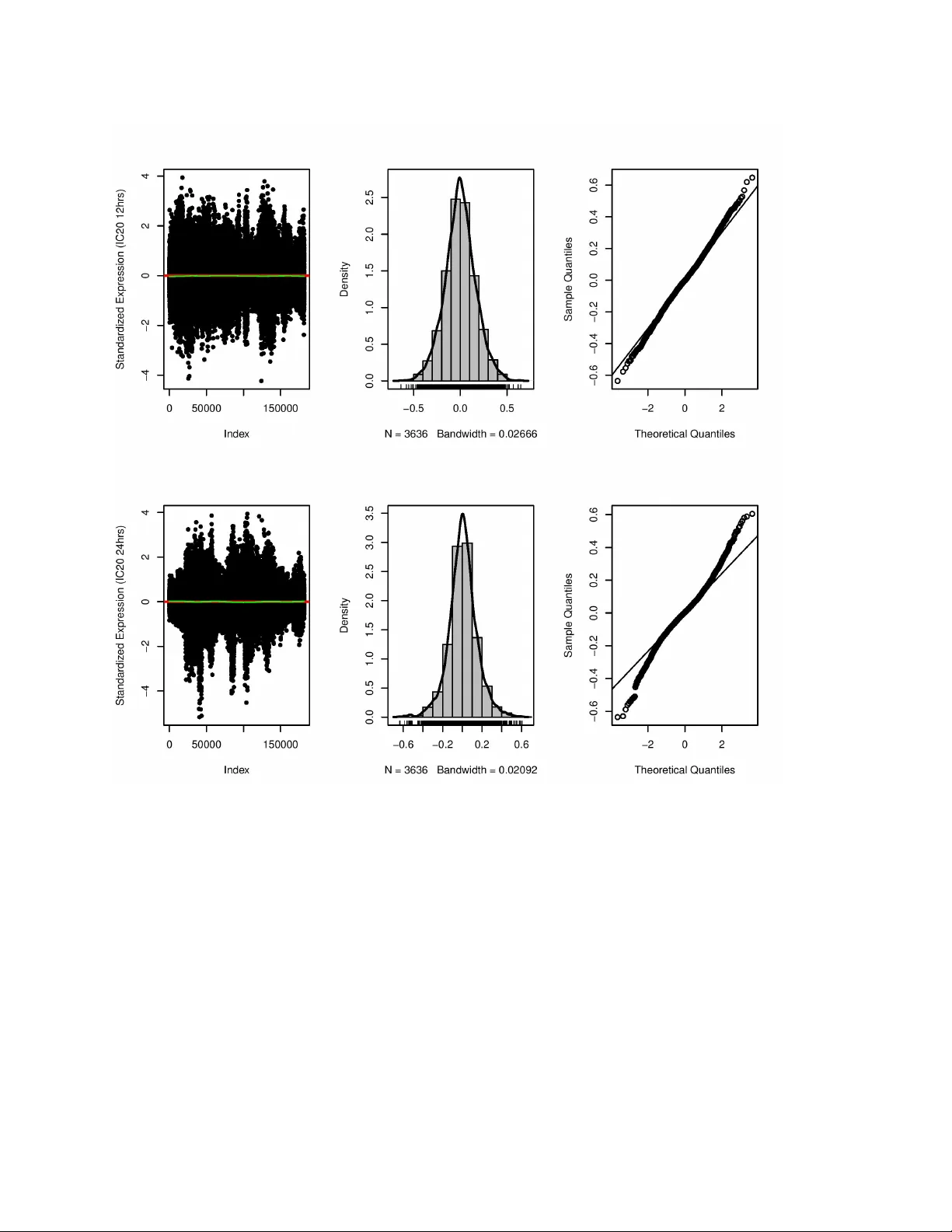
Perturbation Detection Through Modeling of Gene Expression on a Latent Biological P athway Netw ork: A Bayesian hierarchical approach Lisa M. Pham Luis Carv alho Scott Schaus Eric D. K olaczyk Boston Uni versity , Boston, MA 02215 email: lisamlpham@gmail.com August 20, 2021 A uthor’ s F ootnote: This research was supported, in part, by NIH grant GM078987. EK is partially supported by AFOSR grant 12RSL042. LC is supported by NSF grant DMS-1107067. LP is supported by NIH/NIDDK grant R01 DK078616. Mailing address: Program in Bioinformatics, Boston Uni versity , 24 Cummington Street, Boston, MA 02215 (email: lisamlpham@gmail.com). 1 Abstract Cellular response to a perturbation is the result of a dynamic system of biological v ariables linked in a complex network. A major challenge in drug and disease studies is identifying the key factors of a biological network that are essential in determining the cell’ s fate. Here our goal is the identiﬁcation of perturbed pathways from high-throughput gene expression data. W e dev elop a three-lev el hierarchical model, where (i) the ﬁrst level captures the relationship between gene expression and biological pathw ays using conﬁrmatory factor analysis, (ii) the second le vel models the beha vior within an underlying network of pathways induced by an unknown per- turbation using a conditional autoregressiv e model, and (iii) the third level is a spike-and-slab prior on the perturbations. W e then identify perturbations through posterior-based v ariable selection. W e illustrate our approach using gene transcription drug perturbation proﬁles from the DREAM7 drug sensitivity predication challenge data set. Our proposed method identiﬁed regulatory path- ways that are known to play a causativ e role and that were not readily resolved using gene set enrichment analysis or exploratory factor models. Simulation results are presented assessing the performance of this model relative to a network-free v ariant and its robustness to inaccuracies in biological databases. K E Y W O R D S : Bayesian F actor Models, Conﬁrmatory Factor Analysis, Conditional Autoregressi ve Models, MCMC, Network Biology , Drug T ar get Prediction, Microarray 1. INTRODUCTION W ith the inﬂux of high-throughput genomic data, understanding biological mechanisms of action that cause changes in cellular homeostasis has become a reachable challenge in the ﬁelds of bioin- formatics, computational biology , and statistics. High-throughput measurement techniques such as transcriptional proﬁling allow us to measure gene transcript le vels across thousands of genes si- multaneously . Ho we ver , analyzing individual gene transcriptional proﬁles, cannot, by themselves, elucidate biological mechanisms that are responsible for the changes observed in gene e xpression. Rather , gene transcription provides only one facet of a multif aceted system of biological v ariables that culminate to form a cellular response. Mechanisms of action (MoA) that driv e cellular dysregulation can arise in sev eral biological contexts. Chemotherapeutic compounds for instance, alter very distinct mechanisms, such as chang- ing the topology of DN A structure induced by speciﬁc topoisomerase inhibitors (e.g. (Malik et al., 2006; Nakada et al., 2006)), or inhibiting cellular motility mechanisms caused by myosin II inhibitor compounds (e.g. (Allingham et al., 2005)). In another example, cancer metastasis is also caused by aberrant pathways that disrupt normal cellular regulation, resulting in cancer proliferation. The identiﬁcation of such key mechanisms is important as they can provide unique signatures not read- ily apparent by directly analyzing gene e xpression without added structure or biological context. Methods that le verage biological information by incorporating added structure or biology can be used as a diagnostic tool in a clinical context. Our primary goal in this paper is to identify drug targets and mechanisms of action in drug perturbation experiments. That is, we aim to ﬁnd pathways signiﬁcantly related to each drug’ s MoA, which can enhance both therapeutic beneﬁt and assessment of efﬁcacy . Moreov er, understanding a drug’ s MoA and biological pathway information can provide a better assessment of cellular response to drugs, possibly providing a therapeutic proﬁle for each drug selection. 2 1.1 The drug target problem: an inv erse problem A cellular response is the result of a culmination of interactions between genes/proteins. A single perturbed pathway , for instance, can cause a rippling effect across a global network of interactions, leaving behind a cascade of transcriptional dysregulation across the genome. F or instance, Fig. 1 is a schematic illustration of ho w a drug perturbs a system of interacting pathways. In Fig. 1, the inhibition/acti v ation of a protein (s) in a single pathway consequently alters sev eral downstream pathways, leading to changes in gene expression. T o better understand the primary targets of a perturbation source, we propose a method that formally ﬁlters out these regulatory dependencies between biological factors (pathways) to uncover the primary target underlying a perturbation re- sponse. [Figure 1 about here.] From a mathematical perspectiv e, the nature of the problem we address in this paper is not unlike that of ‘decon volution’ in image processing, a similarity that has been noted by others in this area (e.g., ‘drug target decon volution’ (T erstappen et al., 2007)). In the image processing version of this problem, an image, say f , is of interest but one has av ailable only blurred and noisy measurements, say y = K f + e . While denoising y can be relati vely straightforward, it only leaves one with an estimate of the blurred image, K f . In order to reco ver f itself, the ef fect of the blurring operator K must be in verted. Ho wev er , ev en in the ideal case where K is kno wn this in version can be ill-posed and the reco very of f can be se verely de graded by the corresponding inﬂation of the noise e . When K is unkno wn or only partially kno wn, as is analogous to what we face in the drug target prediction problem, the degradation can be arbitrarily w orse. 1.2 Identifying P athwa y T argets in the DREAM 7 Drug Sensitivity Prediction Challenge Data Set For our purposes of target pathway identiﬁcation in drug perturbation experiments, we e xplore the NCI DREAM7 drug sensiti vity prediction challenge dataset (Bansal et al., 2014) which is a part of the Dialogue for Re verse Engineering Assessments and Methods (DREAM) challenge series (Marbach et al., 2012; Prill et al., 2011). T o assess the performance of our method, we focus our attention on the DREAM7 drug sub-challenge 2 dataset (Bansal et al., 2014) which consists of microarray gene expression proﬁles from the L Y3 cancer cell line. Exactly 14 drugs were tested at dif ferent concentrations and durations, and were compared to their mock control counterparts. These high quality , methodical, and carefully designed experiments serve well in testing methods that are designed to predict drug mode of actions because their cellular effects hav e been well studied, spanning a variety of mechanisms from DNA-damaging agents (e.g. etoposide (Nakada et al., 2006)) or cellular motility inhibitors (e.g. blebbistatin (Allingham et al., 2005)) to compounds that disrupt regulatory signaling mechanisms (e.g geldanamycin (Neckers et al., 1999; Grenert et al., 1997)). Dif ferential gene expression analyses and other gene enrichment methods may provide insight into dysregulated genes or gene sets (e.g. biological pathw ays) resulting from a drug perturbation propagating through a system of interacting genes or proteins. Howe ver , identifying the primary source of perturbation that can explain the global variation in gene expression is often dif ﬁcult to discern from differential gene expression alone. For instance, DNA damaging agents that induce cell cycle arrest initiate a series of biological processes such as cell death pathways (apoptosis), protein degradation pathways (e.g. RN A de gradation, ubiquitin mediated proteolysis), and possibly DNA- repair pathways. As a result, genes associated with these downstream pathways may be upre gulated and consequently , identiﬁed by differential gene analyses such as gene set enrichment analysis (GSEA, Subramanian et al., 2005). Rather than detecting the residual ef fects of such a perturbation, 3 we aim to identify upstream pathw ays positioned to cause changes in gene expression. In fact, in the case of DN A damaging agents such as the drug camptothecin, we identiﬁed P53 signaling in the DREAM7 dataset while GSEA has not (see Section 6.4 for details); P53 signaling may be causally linked to cell cycle arrest induced by DN A damage (Jaks et al., 2001; Gupta et al., 1997; W ang et al., 2004). Moreov er, comparing drug proﬁles from two dif ferent exposure times, we sho w that certain drugs are more sensiti ve on the L Y3 cancer cell line than others. W e also identiﬁed drug-induced pathways that were consistently identiﬁed across varying conditions. Lastly , we found that drugs having similar mechanisms (e.g. DN A damaging agents) clustered together using proﬁles generated by our method. 1.3 Organization of this paper In Section 2, we discuss related work. In Section 3, we describe the hierarchical model in detail including priors and model identiﬁcation constraints. In Section 4, we outline the aims of posterior inference and the steps to our sampler . W e assess the performance of our model compared to an exploratory factor analysis (EF A) model using simulated data sets in Section 5. W e discuss our results after applying our method to a drug perturbation dataset (DREAM7 (Bansal et al., 2014)) and compare our method against an EF A model and gene set enrichment analysis (GSEA) (Subramanian et al., 2005) in Section 6. Lastly , in Section 7, we summarize our method as well as our results. 2. PRIOR AND RELA TED WORK Currently , there are roughly three ways the task of identifying disease or drug targets ha ve been approached. In the simplest approach, statistical methods are used to ﬁnd differential expression between a binary phenotype (Dudoit et al., 2003; Storey and T ibshirani, 2003). The goal with this approach is to identify indi viduals genes whose expression le vels are associated with a trait relati ve to some control conditions. These methods are rooted in multiple testing and usually control either the family-wise error rate (Dudoit et al., 2003) or the false discovery rate (Dudoit et al., 2003; Storey and T ibshirani, 2003). Although relati vely straightforward, these methods hav e two main drawbacks: they can only identify do wnstream transcriptional effects since the goal is to detect dif ferential expression and not possible sources of perturbations; and they operate on a gene-by- gene basis and so the phenotypes for each gene are compared in isolation instead of in coordination across gene sets. The second approach, howe ver , uses biological information to group genes with the goal of capturing coordinated expression changes within a gene set that might not have been detected if the analysis were conducted in individual genes. The aim, therefore, is to look for statistical sig- niﬁcance in differential expression across entire gene sets. These gene sets represent a system’ s le vel vie w of the cell such as cellular pathways or transcription factor targets. The most simple and straightforward method to test if a gene set contains a signiﬁcant amount of transcriptionally altered genes is a hyper geometric test. This method and other similarly straightforward methods are re vie wed in (Khatri and Draghici, 2005; Ri v als et al., 2007). Subramanian et al. (2005) de veloped a method called gene set enrichment analysis (GSEA) with the same goal, b ut this method does not re- quire a user to choose a threshold to separate differentially e xpressed genes from non-differentially expressed genes. Instead, GSEA measures how well a gene set clusters at the top or bottom of a rank ed list of genes (e.g. ranked using fold ratios or p-values from two sample tests when comparing binary phenotypes). Extensions of GSEA and other threshold-free methods are described in (Jiang and Gentleman, 2007; Nam and Kim, 2008). GSEA is the most widely used gene set analysis tool to date, ho we ver it does not use an y gene network information. The third and ﬁnal approach is network-based and uses information from cellular regulation or 4 gene-protein interactions to pro vide a better understanding of the molecular mechanisms underlying a response. On an individual protein-gene lev el, many supervised methods hav e been proposed to predict interactions between drugs and proteins. For instance, using existing information of known protein-drug interactions, machine learning methods (Faulon et al., 2008; Y amanishi et al., 2008) hav e been used to predict interactions of individual proteins and drugs using a combination of pro- tein sequence and chemical data. Network based approaches that identify gene sets over indi vidual genes or proteins hav e also been proposed. Gu et al. (2010), for instance, use a two step method where in the ﬁrst step the y identify a set of dif ferentially expressed (DE) genes that are then mapped to a biological network; in the second step, a clustering method is used to identify genes that form a connected subgraph of DE genes. Other techniques, including pathway-e xpress (Draghici et al., 2007) and gene network enrichment analysis (Liu et al., 2010) have also used network topology . Pathw ay-express (Draghici et al., 2007) scores genes in a network using differential expression such that differentially expressed genes that are connected are scored higher than those that are not connected. Pre-deﬁned gene sets are then represented using the scores of its genes in the net- work. Gene network enrichment analysis (Liu et al., 2010) ﬁrst identiﬁes a connected subnetwork of dif ferentially expressed genes of a global protein-protein interaction netw ork, and then identiﬁes pre-deﬁned gene sets, such as biological pathways, that are enriched with respect to the genes in a dif ferentially expressed subnetw ork. Although these increasingly complex approaches serve well in identifying genes or gene sets that are differentially expressed, they are not designed to identify which genes or gene sets, of the collection of genes or gene sets identiﬁed by their method, are primary targets of a speciﬁc response, and thus they do not prescribe a mechanism of action. T o this end, it is essential to explicitly model the cascading ef fects of a perturbation by considering biological relationships in a gene network. Our proposed method is such a model-based approach: a factor model, called conﬁrmatory factor analysis (CF A) with a conditional autoregressi ve (CAR) component designed to identify primary targets underlying gene expression. Spatial conditional autoregressi ve models hav e recently been explored in biology , speciﬁcally with functional networks (e.g. (W ei and P an, 2008)). The motiv ation behind such models stems from the principle that genes that work together (i.e. genes that are functionally related) are usually co-expressed/inhibited, co-(de)regulated, or co- (de)acti v ated. Factor analysis models hav e also been used e xtensi vely in biology (Lucas et al., 2006; Carvalho et al., 2008; Lucas et al., 2010; Ma and Zhao, 2012). Ma and Zhao (2012) use a Bayesian factor analysis model to identify drug-pathway interactions by analyzing paired gene e xpression and drug sensiti vity data and their relationship to common pathways, represented as latent factors. In their model all factors (pathways), howe ver , are independent. These network-free models are referred to as exploratory factor analysis (EF A) models. W est et al. (Lucas et al., 2006; Carvalho et al., 2008) also uses exploratory factor analysis models but with an aim to identify biomarkers using gene expression data. Ho wev er, in (Lucas et al., 2006; Carv alho et al., 2008) the factors are not structurally informed by kno wn biological gene sets and instead are completely data-dri ven. Lastly , EF A or traditional CF A models assume a zero prior mean for the latent factors. Con versely , our proposed method is a nov el approach to perturbation target identiﬁcation on a latent scale which giv e rise to non-tri vial prior means on the latent f actors. T ogether , our proposed method is a synthesis of se veral ke y principles from both conﬁrmatory factor models and conditional autoregressi ve models that allow us to explain the variation observed in transcriptional data as a function of perturbations to a latent network of biological pathways. Our proposed model was ﬁrst motiv ated by the w ork of di Bernardo et al. (2005), where a math- ematical model adapted from Hill-type transcription kinetics (Liao et al., 2003) was used to describe the relationships among gene transcripts in a cell. The model captures both internal regulatory in- 5 ﬂuences among p gene transcripts and ef fects due to external perturbation ef fects: log 10 ν i ν ib ! = log 10 µ i µ ib ! + p X j =1 η ij log 10 ν j ν j b ! , (1) where ν i , for i = 1 , . . . , p , represents the expression le vel of transcript i , µ i represents the direct inﬂuence of the perturbation on transcript i , ν ib and µ ib represent a set of baseline v alues of ν i and µ i , respectiv ely , and η ij represents the inﬂuence of transcript j on transcript i . This can be re-expressed as ψ = B ψ + φ (2) where ψ = ( ψ 1 , . . . , ψ p ) 0 with ψ i = log 10 ( ν i /ν ib ) , and φ = ( φ 1 , . . . , φ p ) 0 with φ i = [1 / (1 − η ii )] log 10 ( µ i /µ ib ) , a scaled v ersion of the log-relati ve direct inﬂuence of the perturbation. Here, B is a p × p matrix representing the network interaction effects among gene transcripts with B ii = 0 and, for i 6 = j , B ij = η ij / (1 − η ii ) . The work in (Cosgrove et al., 2008) is a statistical extension of the mathematical model in Eq. (2) in the form of y = B y + φ + e (3) where y is no w the p × 1 vector of measures of ψ . Here, each measured e xpression lev el y i is poten- tially inﬂuenced by other transcripts, where this inﬂuence is captured through B . The perturbations are additi ve components represented by φ . Here, we further extend this model to factor analysis models which are frequently used to an- alyze high-dimensional gene expression data (Ma and Zhao, 2012; Lucas et al., 2010; Carvalho et al., 2008; Lucas et al., 2006). Here, we assume that gene expression is linked to an o verall factor deﬁned by biological pathways in the cell. Our proposed model can be described as a hierarchical model where the ﬁrst (gene) lev el is a regression of gene expression on biological pathways, and the second (pathw ay) le vel is an auto-regressi ve model that models the behavior of a system of interact- ing biological pathways underlying external perturbation ef fects. W e describe the proposed model in Section 3. 3. MODEL FRAMEWORK W e de veloped a statistica l hierarchical model to uncov er perturbations to biological pathways using high-throughput measurements of gene e xpression on individual genes. The data Y = { Y e , Y c } is a p × n matrix of transcriptional proﬁles of p genes across n varying conditions, and consists of a set of cases, Y e , and controls, Y c . T o av oid using an intercept in our model, we center the data with respect to the mean of the control group, Y c . Our goal is to identify latent factors (e.g. biological pathways) that can explain the v ariation observ ed in the experimental data, Y e , relati ve to the control conditions, Y c . Our model is built on three hierarchical components: y ki | Λ , ω i , ψ k ind ∼ N (Λ k ω i , ψ k ) (4) ω j i | ω [ − j ] i , ρ j i , σ 2 ind ∼ N q X j 0 =1 ,j 0 6 = j B j j 0 ω j 0 i + ρ j i , σ 2 ! (5) ρ j i | θ j i , τ 2 ind ∼ N (0 , θ j i τ 2 + (1 − θ j i ) v 0 τ 2 ) (6) for i = 1 , . . . , n , k = 1 , . . . , p , j = 1 , . . . , q , where n , p , and q represent the number of samples, genes, and pathways, respecti vely , and 6 • y ki is the observed gene e xpression level of gene k in sample i . • ω i is a q × 1 v ector of latent common factors representing inherent pathw ay ef fects for sample i . • Λ is a p × q factor loadings matrix in the CF A model, relating gene expression to pathway ef fects. Λ k is the k -th row of Λ . • ρ j i is a random “external” perturbation ef fect for pathway j in sample i . • θ j i is an indicator for pathway j in sample i being perturbed. W e describe and motiv ate the v arious aspects of this model in more detail in the follo wing subsections. 3.1 Modelling Biological Replicates It is common in biological studies to have replicates. In this case we allow perturbations and latent factors to v ary for each replicate, yielding the model y kir | Λ , ω ir , ψ k ind ∼ N (Λ k ω ir , ψ k ) (4’) ω j ir | ω [ − j ] ir , ρ j ir , σ 2 ind ∼ N q X j 0 =1 ,j 0 6 = j B j j 0 ω j 0 ir + ρ j ir , σ 2 ! (5’) ρ j ir | θ j i , τ 2 ind ∼ N (0 , θ j i τ 2 + (1 − θ j i ) v 0 τ 2 ) (6’) for replicates r = 1 , . . . , m i in each study . Note that while ρ and ω vary , we assume the same perturbation targets and gene-pathw ay loadings across replicates and so θ and Λ do not depend on index r . In the ne xt sections we present each of the these lev els in detail, but we drop the replicate indices to simplify the notation. 3.2 Conﬁr mator y F actor Le v el In the ﬁrst component, we focus on the likelihood of individual gene e xpression measurements. It has been sho wn that the transcriptional acti vity of a gene is, in part, regulated by pathways posi- tioned upstream of gene regulation (e.g. (V ogelstein and Kinzler, 2004)). W e describe this rela- tionship between a gene and its pathw ays using a conﬁrmatory factor analysis model, as sho wn in Eq. (4). Here, the gene expression measurements, Y , are regressed on a set of biologically structured latent factors ω (biological pathways). Both the structure of the latent factors ω and the dependency between individual genes y and these latent factors are encoded, a priori, in the p × q loading factor matrix Λ . W e integrate biological information into the model through Λ , by limiting some of the elements of Λ to zero, where the non- zero elements in each column of Λ correspond to the genes of a known canonical pathway . That is, a gene k loads onto a pathway j , (that is, λ kj 6 = 0 ) if gene k (or its gene product) is a member of pathway j . If a gene (or its gene product) is not in a pathw ay , the corresponding loading factor is constrained to 0 . Thus genes are regressed only on the pathways to which the y belong. W e use the following priors for the loading f actors Λ : λ kj iid ∼ ( N (0 , 0 . 1) , if gene k is in pathway j δ 0 ( · ) , otherwise where we set the v ariance of Λ to be small to prev ent the latent factors from shrinking tow ards zero in practice, and keep the pathway noise v ariance weakly informativ e. 7 W e giv e the gene variances Ψ in verse g amma priors, ψ k iid ∼ IG ( ζ , ζ − 1) , k = 1 , . . . , p, where the shape is chosen so that the prior mean is 1 . W e now control the prior strength of the gene noise v ariance parameters Ψ through the hyper-parameter ζ to avoid ov erﬁtting the model. This prior regularization is important in cases where the data size is not large enough to ﬁt com- plex hierarchical models and can lead to instability , poor con ver gence, multiple local modes, and empirically non-identiﬁed models when the prior on each ψ k is too ﬂexible. The e xtent to which an in verse gamma prior is informativ e depends on the strength of the data and is translated as a v ariance tradeof f between the prior and the data in the conditional posterior distribution of ψ k : ψ k | Ω , Λ , Y ∼ IG ζ + n 2 , ζ − 1 + 1 2 n X i =1 ( Y ki − Λ k, · ω i ) 2 ! . (7) Since an in verse gamma distribution with shape α corresponds to a χ 2 distribution with 2 α degrees of freedom (Gelman, 2006), the prior provides 2 ζ pseudo-observ ations and the conditional in (7) has 2 ζ + n observ ations. W e thus constrain the prior variances of Ψ by setting κ times data observ ations as prior pseudo-observations, ζ = κn/ 2 , and so the conditional in (7) has n ( κ + 1) degrees of freedom. In this manner , we ﬁx κ < 1 so that the prior does not ov erpower the likelihood. In our implementation, we ﬁxed κ to 0 . 5 to ha ve a reasonably informed prior . 3.3 Conditional A utoregressive Le vel The second component of the model is designed to characterize a perturbed system of interacting pathways. The dependency between pathways is captured by a conditional autor e gr essive model (Cressie, 1993; de Oliveira, 2012) in Eq. (5). The reasoning is that, under normal stationary condi- tions, each pathway can be explained, on a verage, by other pathw ays in a pathway-pathway network through the coefﬁcients B . Howe ver , when a pathway is targeted by some external perturbation source (e.g. from disease, or drug perturbation), then the expected mean of this pathway is shifted by an additional term ρ due to the perturbation. In the context of drug perturbations, one can effec- ti vely imagine that after a drug hits a speciﬁc pathway , this drug-induced ef fect propagates across the network, af fecting many pathways by mere association, and altering cellular phenotype. In the CAR lev el of the model, Eq. (5), the q × q design matrix B represents a system of pathway-pathway interactions. More speciﬁcally , let us initially set B := γ W , where γ is referred in the CAR literature as the spatial scaling parameter, and W is a symmetric zero-diagonal matrix. W e brieﬂy describe the pathway network W in Section 3.4 and provide a technical description in Appendix A. If we deﬁne Φ := ( I − γ W ) − 1 , where I represents the identity matrix of order q , the joint distribution of ω can be written as the following (Cressie, 1993): ω | ρ, Φ , σ 2 ∼ N (Φ ρ, σ 2 Φ) . (8) Thus, if γ = 0 the CAR model is reduced to an exploratory factor analysis model. Ho we ver , to attain an identiﬁable model (please refer to Section 3.6 for details), we require that the factors have equal v ariance s 2 and so Φ = s 2 R ( γ ) , where R ( γ ) is the correlation induced by G ( γ ) := ( I − γ W ) − 1 , R ( γ ) = Diag ( G ( γ )) − 1 2 G ( γ ) Diag ( G ( γ )) − 1 2 . (9) In addition, to ensure that Φ is positiv e deﬁnite, we constrain γ to the interval (1 /ι 1 , 1 /ι q ) , where ι 1 and ι q are the minimum and maximum eigen v alues of W , respectiv ely . The prior on γ is 8 uniform, γ ∼ Unif 1 ι 1 + δ, 1 ι q − δ ! , where δ > 0 ensures that the maximum correlation in R ( γ ) is not near 1 , which can lead to a non- identiﬁed model. W e set δ = 0 . 005 , which, in our experience, bounds the maximum correlation at roughly 0 . 90 . Finally , we set a weakly informati ve prior on σ 2 , σ 2 ∼ IG (0 . 001 , 0 . 001) . 3.4 Interaction Network in the CAR Model The pathway interaction network lies at the core of our model. W e speciﬁcally use a network, where nodes are pathways, constructed in a manner that implicitly links pathways by their common function in the cell. T o date there are several ways of building a pathway interaction network. The most ad-hoc approach is to simply deﬁne a link between two pathways where there is a non- empty intersection of gene members. Howe ver , this rule ov erlooks interactions that may occur between non-overlapping genes of two pathways. An alternative approach is to use a protein-protein interaction database to identify physical interactions between members of two pathways, and using an aggregate score to deﬁne the ov erall interaction link. Howe ver , using PPI interactions is often very noisy giv en the high variability in PPI data (von Mering et al., 2002; Reguly et al., 2006; Gandhi et al., 2006) resulting from methods that produce high-cov erage of the proteome inherently having a high f alse positive rate. T o better capture interactions between pathways, we used Gene Ontology’ s (GO) biological processes (The Gene Ontology Consortium, 2000) to deﬁne functional links between pathways. The adv antage of GO ov er a PPI database is that a GO gene set is manually curated, thus containing much fewer false positiv es. Functional networks hav e been used extensi vely in biology (Ideker et al., 2002; Chuang et al., 2007; Rogue v et al., 2008), which are generally motiv ated by the principle that genes that work together to accomplish a task in the cell are usually co-acti vated/inhibited or co- (de)regulated. T o construct the pathway-pathway interaction network W , we regard the set of pathways as a weighted network where the nodes represent canonical pathways and the edge weights in W reﬂect the degree of functional similarity between two pathways. As an example, in Fig. 1 the nodes would represent P athways A, B, and C with a link connecting Pathways A to B and A to C. W e then create W in a manner similar to an algorithm by Pham et al. (2011) using KEGG regulatory and signaling pathways (Kanehisa et al., 2006; Kanehisa and Goto, 2000), and GO biological processes (The Gene Ontology Consortium, 2000) obtained from the MSigDB collection (Subramanian et al., 2005). For a technical description of the network construction see Section A. 3.5 Spike-and-Slab Prior Our goal of elucidating primary targets of a perturbation reduces to identifying perturbation effects after accounting for all pathway-pathw ay interactions (i.e. via network ﬁltering) as described by a kno wn biological network W . Importantly , we assume that relati vely fe w pathways are primary targets of a perturbation. W e use a spike-and-slab prior on ρ (Geor ge and McCulloch, 1997) and identify perturbations through posterior -based variable selection. Thus our parameters of interest are variables θ j i that indicate whether ρ j i represents a non-zero perturbation for pathway j in sample i , as in Eq. (6). Because the scale of the perturbations is unknown, we choose a mixture of two normals (Geor ge and McCulloch, 1997), one approximating the spike and the other the slab, in such a way that is in variant to the scale of the perturbations. That is, we deﬁne the spike variance to be some fraction v 0 of the slab variance (Braunstein et al., 2011) and let the slab variance be random. W e ﬁxed 9 v 0 = 0 . 01 , meaning that a non-perturbed pathway has only one-hundredth of the variance of a perturbed pathway , while keeping the prior on τ 2 weakly informati ve, similarly to the prior on σ 2 . Lastly , the prior probability of a pathway being perturbed is captured by a hyper-parameter α . W e expect α to be small to reﬂect the targeted effect of drug perturbations to a fe w pathways because, for instance, the FD A requires perturbation selectivity for drug approv al. Thus, to induce sparsity we set α = 0 . 1 as an upper bound for the expected fraction of perturbed pathways, yielding: θ j i iid ∼ Ber n (0 . 1) τ 2 ∼ IG (0 . 001 , 0 . 001) , for j = 1 , . . . , q and i = 1 , . . . , n . While we expect a priori that at most 10% of the pathways are selectiv ely perturbed, we found in a prior sensitivity analysis that small changes in α do not signiﬁcantly change our inference on perturbation detection. 3.6 Model Identiﬁcation Model identiﬁcation has always been a non-trivial task with factor models (see Chapters 4, 7, 8 in (Bollen, 1989)). In CF A models, constraints are usually applied to elements of both Φ and Λ . This can be done, for example, by ﬁxing the factor v ariances and the ﬁrst q rows of Λ to a particular structure (Lucas et al., 2006). These methods pre vent non-tri vial rotational or scale transformations of Λ and Φ by forcing the transformation matrix U to be the identity matrix. Howe ver , since in our model Φ := s 2 R , where R is a correlation matrix (Eq. (9)), Φ is already rotationally unique. This model, howe ver , is still not identiﬁed in a few additional ways. Firstly , for the i -th sample we hav e Y i | Λ , ω i , Ψ ∼ N (Λ ω i , Ψ) and so, if we marginalize ω i we hav e the following conditional distribution on Y i : Y i | Λ , ρ i , σ 2 , γ , Ψ ∼ N ( s 2 Λ R ( γ ) ρ i , Ψ + σ 2 s 2 Λ R ( γ )Λ > ) . (10) Thus, if we re-scale e σ 2 = k σ σ 2 , e s 2 = k s s 2 , e ρ i = k ρ ρ i , and e Λ = k Λ Λ such that k s k Λ k ρ = 1 and k σ k s k 2 Λ = 1 we obtain the same conditional distribution on Y i since its mean and variance remain unaltered, respecti vely . For example, re-scaling Λ , σ 2 and ρ i with any scalar a 6 = 0 such that e Λ = a Λ , e σ 2 = σ 2 /a 2 , and e ρ i = ρ i /a does not affect the distribution of Y i . T o solve these forms of re- scaling, we ﬁx s 2 = 1 as well as the prior variance of Λ to 0 . 1 , a small value that avoids shrinking the scale on ω towards 0 in practice. Finally , there is an additional case that can lead to a non-identiﬁed model. This last case arises from the latent factor correlation matrix R . In the simplest case, suppose γ 6 = 0 and W is a connected network (i.e. R can only be arranged as a single block matrix). Under these conditions, there exist e xactly two solutions where e Λ = − Λ , e ω = − ω , e ρ = − ρ. This is simply a sign ﬂip across all pathways, which would not affect the underlying factor cov ariance structure Φ . In fact, if R is rearranged into a block diagonal matrix, then each set of pathways corresponding to a block in R can be ﬂipped in this manner without affecting Θ and yielding the same joint posterior density . In other words, if R is rearranged into a block diagonal matrix with b blocks then there exist e xactly 2 b solutions. Therefore, perturbations are identiﬁed up to their signs; that is, we can infer if two pathways are perturbed in the same direction, but if the perturbation is positi ve or ne gati ve is arbitrary . Moreov er , since our goal is to infer perturbations, 10 we are more interested in the magnitude of a perturbation—whether it is signiﬁcantly close to zero or not—rather than its sign. 4. POSTERIOR INFERENCE Our primary goal is the posterior inference on Θ = { θ j i } , which is used to identify perturbation targets. W e obtained posterior estimates to our model parameters via a partially collapsed hybrid Gibbs sampler (van Dyk and Park, 2008) with an adapti ve Metropolis step (Gelman et al., 2004). W e call the sampler “partially collapsed” because we sample some of the parameters (namely , ρ and θ ) from a mar ginalized conditional posterior . W e found that using this partially collapsed sampler facilitates the sampler to mo ve into re gions of high posterior mass concentration faster . First, the steps for an ordinary , non-collapsed Gibbs sampler (dropping iteration indices and irrele v ant conditional parameters) are: [Λ | ω , ψ , Y ] , [ ρ | θ , Φ , ω , σ 2 , τ 2 ] ∗ , [ θ | ρ, τ 2 ] ∗ , [ γ | ω , ρ, Φ , σ 2 ] , [ ω | Λ , ρ, ψ , Φ , σ 2 , Y ] , [ ψ | Λ , ω , Y ] , [ σ 2 | ω , ρ, Φ] , [ τ 2 | ρ, θ ] . Note that, ev en though Φ = s 2 R ( γ ) is a matrix that depends on γ , we use them interchangeably to make the conditional distributions clearer . Now , to improve the rate of con vergence, we mar ginalize the two steps starred above: (i) instead of sampling from [ ρ | θ , Φ , ω , σ 2 , τ 2 ] , we integrate out ω from [ ρ, ω | Λ , θ, Φ , ψ , σ 2 , τ 2 , Y ] ; and (ii) instead of sampling from [ θ | ρ, τ 2 ] , we marginalize ρ from [ θ , ρ | ω , Φ , τ 2 , σ 2 ] . The collapsed sampler has then updated steps [ ρ | Λ , θ , Φ , ψ , σ 2 , τ 2 , Y ] and [ θ | ω , Φ , τ 2 , σ 2 ] . W e note that, as v an Dyk and Park (2008) pointed out, marginalizing does not alter the stationary distribution of the full posterior nor the compatibility of the conditional distributions. In the next sections we provide details on each of these steps. 4.1 Initializing MCMC chains W e implemented a tempering algorithm at the beginning of our MCMC chains to ﬁnd reasonable starting points such that the chains were less likely to get stuck at a local mode. These local modes are caused, in part, by each lik elihood in the CF A le vel, Eq. (4), being close to non-identiﬁable up to the mean Λ ω . T o do this, we run our sampler as usual, but for Ψ , Λ , and Ω , we temper the likelihood distributions Y | Ψ , Λ , Ω when obtaining their conditional posteriors. Similarly , we do the same for the likelihood of Y | ρ when sampling ρ . At hot temperatures, the likelihood of Y would be ﬂatter, allo wing the chains to move more freely around the space. W e slo wly cool the temperature to T = 1 to obtain the targeted posterior and thus be ginning the true sampler . 4.2 Sampling Λ Recall that we have constrained some elements in Λ to 0 such that genes are regressed only on pathways to which the y belong. That is, if gene k is not in pathw ay j , then we constrain the element λ kj to 0 . Consider the k -th row of Λ , which we denote as Λ k , and suppose some of the elements in Λ k are constrained to zero. Let c k be the corresponding 1 × q ro w vector such that c kj := I ( gene k 6∈ pathw ay j ) , that is, c kj = 0 if λ kj is a structural zero and so λ kj iid ∼ N (0 , (1 − c kj )0 . 1) . If r k = P j c kj is the number of pathways containing gene k and Λ ∗ k is the 1 × r k ro w vector that contains the unknown 11 parameters in Λ k then the prior on Λ ∗ k is N (0 , H k ) where H k = 0 . 1 I , I the identity matrix of order r k . Similarly , let Ω ∗ k be the r k × n sub-matrix of Ω such that for j = 1 , . . . , r k , all the rows corresponding to c kj = 0 are deleted and also let Y k, · be the 1 × n vector of observ ations for gene k . Then, from a well kno wn result of Lindley and Smith (1972), the posterior conditional distribution for Λ ∗ k , k = 1 , . . . , p , is Λ ∗ k | Y k , Ω ∗ k , ψ k ∼ N ( A − 1 k a k , A − 1 k ) where A k = ψ − 1 k Ω ∗ k Ω ∗ k > + H − 1 k and a k = ψ − 1 k Ω ∗ k Y > k, · . 4.3 Sampling ρ W e deﬁne Σ( θ i ) as a diagonal matrix whose j -th diagonal element is Σ( θ i ) j j = τ 2 [ θ j i + v 0 (1 − θ j i )] . Then, ag ain exploiting the result of Lindle y and Smith (1972) on the mar ginalized conditional distribution of Y i after integrating out ω i in (10), we sample ρ i from the following conditional posterior distribution: ρ i | θ i , Λ , Ψ , Y i ∼ N ( A − 1 i a i , A − 1 i ) , where A i = Φ > Λ > ( σ 2 ΛΦΛ > + Ψ) − 1 ΛΦ + Σ( θ i ) − 1 , a i = Φ > Λ > ( σ 2 ΛΦΛ > + Ψ) − 1 Y i . 4.4 Sampling θ As in the pre vious section, we compute the mar ginalized conditional posterior of θ after inte grating out ρ . For computational efﬁcienc y , we store the mar ginal variance V ( θ ( t ) i ) of ω i conditional on θ i at each iteration t of our sampler , where index i runs over samples. That is, V ( θ i ) = σ 2 Φ + ΦΣ( θ i )Φ > . T o simplify the notation, we drop the sample index i on all parameters including θ . At this step we sample iterati vely from θ j | θ [ − j ] , ω , Φ , τ 2 for j = 1 , . . . , q . There are then two cases: when θ ( t ) j = 0 and when θ ( t ) j = 1 , for which we deﬁne V 0 = V ( θ ( t ) j = 0 , θ ( t ) [ − j ] ) and V 1 = V ( θ ( t ) j = 1 , θ ( t ) [ − j ] ) . Let φ j denote the j th column of Φ . If θ ( t ) j = 0 , then we deﬁne δ j 0 = 1 + ( τ 2 − v 0 τ 2 ) φ > j V − 1 0 φ j and ∆ j 0 = ( τ 2 − v 0 τ 2 ) /δ j 0 ( V − 1 0 φ j )( V − 1 0 φ j ) > to obtain: logit P  θ ( t +1) j = 1 | θ [ − j ] , ω , Φ  = − 1 2 log δ j 0 + 1 2 ω > ∆ j 0 ω + logit ( α ) . If θ ( t ) j = 1 we deﬁne, similarly , δ j 1 = 1 − ( τ 2 − v 0 τ 2 ) φ > j V − 1 1 φ j and ∆ j 1 = ( τ 2 − v 0 τ 2 ) /δ j 1 ( V − 1 1 φ j )( V − 1 1 φ j ) > to obtain: logit P  θ ( t +1) j = 1 | θ [ − j ] , ω , Φ  = 1 2 log δ j 1 + 1 2 ω > ∆ j 1 ω + logit ( α ) . For the full deri vation of these posterior probabilities, please refer to Appendix B. 4.5 Sampling γ As with most spatial models, the scaling parameter γ lacks conjugacy . W e used a random walk adapti ve Metropolis algorithm such that the proposal density is normal and centered at the current 12 sample, γ ( t ) , with variance ξ 2 . This v ariance is tuned to adjust for the acceptance rate and ﬁx ed post burn-in. W e propose γ ∗ ∼ N ( γ ( t ) , ξ 2 ) . Let Φ ∗ = s 2 R ( γ ∗ ) with the correlation computed as in Eq. (9). Then, if l (Φ) := − n 2 log | Φ | − 1 2 n X i =1 ( ω i − Φ ρ i ) > ( σ 2 Φ) − 1 ( ω i − Φ ρ i ) , the acceptance ratio of the Metropolis step is just r ( γ ∗ , γ ( t ) ) = exp { l (Φ ∗ ) − l (Φ ( t ) ) } since we hav e a ﬂat prior on γ . 4.6 Sampling ω , ψ , σ 2 , and τ 2 W e sampled ω according to the linear conditional posterior: ω i | Y i , Λ , Ψ , ρ i , γ ind ∼ N ( A − 1 i a i , A − 1 i ) where A i = Λ > Ψ − 1 Λ + σ − 2 Φ − 1 a i = Λ > Ψ − 1 Y i + σ − 2 ρ i . The conditional distributions of v ariance parameters ψ and σ 2 follo w from conjugacy: ψ k | ω , Λ , Y ∼ IG ζ + n 2 , ζ − 1 + 1 2 n X i =1 ( Y ki − Λ k, ω i ) 2 ! σ 2 | ω , Φ , ρ, ∼ IG 0 . 001 + q n 2 , 0 . 001 + 1 2 n X i =1 ( ω i − Φ ρ i ) > Φ − 1 ( ω i − Φ ρ i ) ! . where ζ = n/ 4 according to the discussion in Section 3.2. The conditional distrib ution of τ 2 is also conjugate; if v ij = 1 when θ ij = 1 and v ij = v 0 when θ ij = 0 , then τ 2 | ρ, θ ∼ IG 0 . 001 + q n 2 , 0 . 001 + q X i =1 n X j =1 ρ 2 ij 2 v ij ! . 4.7 P osterior Inference W e infer perturbations based on the centroid estimator of θ for some threshold t (Carv alho and Lawrence, 2008): b θ j i ( t ) := I  P ( θ j i | Y ) > t  . (11) W e choose the threshold t by controlling a Bayesian false disco very rate. W e deﬁne the Bayesian false disco very rate (BFDR) of an estimator as BFDR ( b θ ( t )) := E θ | Y " P n i =1 P q j =1 b θ j i (1 − θ j i ) P n i =1 P q j =1 b θ j i # = P n i =1 P q j =1 b θ j i (1 − P ( θ j i = 1 | Y )) P n i =1 P q j =1 b θ j i . (12) 13 5. SIMULA TION STUD Y W e conducted a simulation study to (i) assess the impact of including biological network informa- tion into a f actor model, and (ii) test the robustness of our model to inaccuracies in the biological databases used to construct pathways and the pathway-pathw ay interaction network. 5.1 Assessing the impact of incor porating biological network inf or mation W e tested the CF A-CAR model under v arious signal-to-noise (SNR) ratios and compared its perfor- mance with an exploratory factor analysis (EF A) model. This comparison model can be obtained from our original CF A-CAR model, by letting the pathway-pathway network be empty . That is, an EF A model is a factor model such that the factor cov ariance matrix, Φ , is diagonal, which is equi v alent to setting γ = 0 in the CF A-CAR model. In effect, this constraint remov es the netw ork ﬁltering ef fect of the CAR model. The EF A model can thus be written as (Eq. 13): y ki | Λ , ω i , ψ k ind ∼ N (Λ k ω i , ψ k ) (13) ω j i | ω [ − j ] i , ρ j i , σ 2 ind ∼ N ( ρ j i , σ 2 ) (14) ρ j i | θ j i , τ 2 ind ∼ N (0 , θ j i τ 2 + (1 − θ j i ) v 0 τ 2 ) (15) W e simulated toy-scale networks with graph densities similar to the original KEGG pathway network. For each network, we randomly selected q = 10 pathways from our set of KEGG path- ways. In this paper , we describe the results obtained from one of these netw orks. W e obtained the pathway-pathway weighted netw orks by taking the subnetw ork from our original pathw ay-pathway network induced by the ten randomly selected pathways. The number of distinct genes in the union of the selected pathways was 878. W e used the real gene to pathway membership to create the mask of Λ . W e sampled the non-zero loading factors in Λ from a Gaussian with zero mean and v ariance 0 . 1 . The spatial scaling parameter γ was relatively high to emphasize non-trivial links in the network W . W e deﬁne the SNR in each simulated data set using the SNR of a perturbed pathway (which is the same for any perturbed case). If pathway k was perturbed with effect ρ , we deﬁne SNR = ρ/σ , and if we further ﬁx the pathway noise variances ( σ ) to 1 , then the SNR = ρ . In each case sample, we simulated an experiment where only a single pathway was perturbed, with 5 “biological” replicates per experiment (perturbation). Therefore, if we perturbed pathway k in sample i ∈ { 1 , 2 , 3 , 4 , 5 } in experiment j , we set ρ j ki = m , where m is the signal to noise ratio in the data set, and ρ j k 0 i = 0 for k 0 6 = k . Across all data sets, we ﬁxed the gene v ariances ( Ψ ) to 1 . For this network, we created six data sets of different signal to noise ratio in ten simulation replicates. In each data set we ﬁx ed SNR to the following values: 0 . 50 , 1 . 50 , 2 . 50 , 3 . 50 , 4 . 50 , and 5 . 50 . These values were chosen based on the distribution of the SNRs in the NCI-DREAM drug sensiti vity data sets (see Section 6 and Fig. 6). F or each of these data sets, we sampled 50 cases and 50 controls. When running either models, we conditioned the perturbations of all replicates, ρ j i , where j index es the experiment and i index es the experimental replicate, on the same indicator vector θ j . F or the controls, we ﬁx ed the corresponding indicators to zero. W e ran both our CF A model and the EF A model on each data set. Fig. 2 is a series of R OC curves across data sets of different signal to noise ratios. Both models performed similarly under lo w SNRs. Howe ver , the curv es be gin to separate as the signal in the data sets increased. This is further emphasized by the A UC boxplots in Fig. 3. The CF A-CAR model consistently e xhibits a lo w f alse positiv e rate across v arying signal to noise ratios. Unlike the CF A model, the false positive rate of the EF A model increases as the signal to noise ratios increase. When SNR = 4 . 5 the A UC of the EF A model begins to decrease dramatically . This w as 14 expected because giv en a strong enough perturbation, the EF A model confuses a perturbation with the residual do wnstream effects of a perturbation. That is, pathw ays associated with the perturbed pathway are wrongly identiﬁed by the EF A model. [Figure 2 about here.] [Figure 3 about here.] 5.2 Assessing robustness to inaccur acies in the pathwa y database W e performed sensiti vity analysis on the CF A-CAR model to test how possible inaccuracies in KEGG can affect the performance of CF A-CAR relati ve to an EF A model. W ith misannotated genes, the inaccuracy encoded in the mask of Λ would ef fect both the CF A-CAR and EF A models. Ho we ver , inaccuracy in the pathway network would ef fect only the CF A-CAR model. W e provide an example with the same network described in Section 5.1 using a simulated dataset with a signal to noise ratio of 3 . 5 . W e tested six levels of gene set perturbations in the set of pathways, where for each le vel, we randomly perturbed a percentage x of genes. This would ultimately change the loading f actor matrix Λ as well as the pathway-pathway network W . For each lev el, we randomly chose x % of genes represented in KEGG and reassigned them to ne w pathways. W e perturbed x = 1% , 2% , 4% , 8% , 16% , and 32% of all genes in our set of ten pathways. For each of these perturbations, we ran ten replicates where for each replicate we simulated a ne w “pathway” database and ran CF A-CAR on the original data set, using the ne wly constructed Λ and W . Fig. 4 is a series of R OC curves and Fig. 5 are A UC boxplots corresponding to the curves in Fig. 4 for both the CF A-CAR and EF A model across various le vels of gene to pathway reassign- ments. W e begin to see a small departure from the original R OC curve where the network and loading factor matrices were not randomized when 8% of the genes were randomly reassigned to dif ferent pathways. At this le vel, the speciﬁcity of the CF A-CAR model be gins to decrease. How- e ver , even at 32% randomness, the speciﬁcity and sensiti vity of the model is still signiﬁcantly higher than what you expect to see by random chance alone. W e conclude that the CF A-CAR model is rather robust to possible inaccuracies in the biological databases, performing as well or better than an EF A version of this model. [Figure 4 about here.] [Figure 5 about here.] 6. CASE STUD Y : DR UG T ARGET PREDICTION IN DREAM 7 DR UG SENSITIVITY CHALLENGE D A T A W e applied the CF A-CAR model on the NCI-DREAM drug sensitivity challenge data set. As a comparison, we also implemented an EF A model (see Section 5 for a description of the EF A model) and gene set enrichment analysis (GSEA) (Subramanian et al., 2005). The core algorithm of GSEA is a threshold-free variant of a hypergeometric test; howe ver , unlike the CF A-CAR model, network interactions are not used. In the NCI-DREAM drug sensitivity data set, 14 compounds (see T able 1) were tested at v arious concentrations and exposure times on the L Y3 (L ymphoma) cancer cell line. W e focused our atten- tion on the drug data sets with the strongest concentration (IC20) at either 12 or 24 hour e xposures. These data sets were compared to mock control data sets where no drugs were exposed to the cells for 12 or 24 hour durations. There were eight mock replicates and each distinct experiment included three replicates, yielding a total of 50 samples per data set (Data Set 1: IC20 at 24 hours vs Mock at 24 hours and Data Set 2: IC20 at 12 hours vs Mock at 12 hours). 15 [T able 1 about here.] When running CF A-CAR and EF A models, we conditioned the perturbations of all replicates, ρ j 1 , ρ j 2 , ρ j 3 , where j index es the experiment, on the same indicator v ector θ j . In the control cases, we ﬁxed the corresponding indicators θ to 0 . For each dataset, we ran tw o chains of 4000 iterations each, with a burn-in of 2000 . W e assessed conv ergence using the Gelman-Rubin statistic on the absolute values of all the continuous parameters. Fig. 6 summarizes the posterior distributions of the model parameters γ , σ 2 , τ 2 , and the signal to noise ratios (SNRs) across the different drugs for each data set (IC20 at 12 hours and IC20 at 24 hours). W e deﬁne the SNR of a pathway j in a sample i as the mean ratio, across replicates, of the absolute perturbation ρ to either σ , if the pathway is perturbed, or σ √ v 0 otherwise; that is SNR j i = P 3 r =1 ( θ j i | ρ j ir | /σ + (1 − θ j i ) | ρ j ir | / ( σ √ v 0 )) / 3 , where r indexes the replicate of a drug experiment (with 3 replicates per drug). T o assess SNR in a drug case, we pool the signal to noise ratio across all pathways. [Figure 6 about here.] For GSEA, we called a pathway “dysregulated” if the false discovery rate (FDR) adjusted p- v alue is less than 5% . For the CF A-CAR and EF A models we identify perturbations based on the centroid estimator of θ in Eq. (11) where the threshold t was chosen to control BFDR at 5% (see Eq. (12)). Restricting the BFDR at 5% , we used a perturbation threshold of 0 . 72 for IC20 at 12 hours and 0 . 50 for IC20 at 24 hours for the CF A-CAR model. For the EF A model, we used thresholds 0 . 80 and 0 . 70 for IC20 at 12 hours and IC20 at 24 hours, respectively . 6.1 Assessing model ﬁt W e assessed model ﬁt by ﬁrst standardizing the data with respect to its marginalized likelihood gi ven Θ . If, for sample i , Y i | Λ , Φ , θ i , σ 2 , Ψ ∼ N (0 , ΛΦΣ( θ i )Φ > Λ > + σ 2 ΛΦΛ > + Ψ) , then, if C i denotes the Cholesky factor of the abo ve marginalized cov ariance of Y i , we ha ve that Y i ∼ N (0 , C i C > i ) and so e Y i · C − 1 Y i ∼ N (0 , I p ) , where I p is the p -th order identity matrix. Thus, to assess model ﬁt we tak e posterior mean estimates b C i of C i , consider standardized gene e xpressions e Y i = b C − 1 i Y i for each sample i = 1 , . . . , n , and then check two assumptions: zero-mean gene expressions and normality . Figure 7 summarizes our assessment, with samples from IC20 at 12 and 24 hours in top and bottom panels, respectiv ely . In the ﬁrst sub-ﬁgure in the left, we plot pooled standardized gene expressions o ver both samples and genes to assess the zero-mean assumption. As can be seen from the smoother ﬁt, this assumption is well met, but samples might hav e slightly different variance scales. For this reason, since we are focused on gene expressions, we assess normality via av erage standardized gene expressions ov er samples in the two last sub-ﬁgures. W e found that the IC20 at 24 hours data has larger departures from normality in the tails when compared to the IC20 at 12 hours dataset. This departure at IC20 at 24 hours is speciﬁcally due to two of the drugs, H-7 Dihydrochloride (DHCL) and Mitomycin C (MMC), which showed a drastic change in variability between the IC20 at 12 hours and IC20 at 24 hours. This effect is explained in further detail in Section 6.5. [Figure 7 about here.] 16 6.2 Assessing control of f alse positives via cross-v alidation T o verify the accuracy of our method, we tested our model against the control (mock) data by leaving one mock sample (microarray), out of the control group and treated it as a “case”, where the perturbations are left unknown. W e applied this leave-one-out cross-validation to each of the 8 control samples, to verify that the perturbed pathways identiﬁed in the case samples are not similarly identiﬁed against a control sample. W e found that in each leave-one-out cross-v alidation test, we did not identify any pathw ays as being perturbed in the mock sample (Fig. 8). [Figure 8 about here.] 6.3 Comparing EF A and CF A-CAR model results Overall, we found that for both data sets, the EF A model was less sensitive than the CF A model, ﬁnding a subset of mechanistically rele vant pathways that were identiﬁed by the CF A model. Be- cause the EF A model identiﬁed fewer pathways linked to drug mechanisms, we choose to focus our comparison with GSEA in the following subsections. Results obtained from the EF A model can be found in Appendix C. 6.4 IC20 concentration at 12 hours For the CF A-CAR model results, we ran a hierarchical bi-clustering analysis on the posterior means b Θ of Θ . More speciﬁcally , we independently cluster samples (drugs) and pathways using complete linkage and Euclidean distances as dissimilarity metrics. Each dimension has their observations swapped to match the clustering hierarch y , as can be seen in Fig 9A. Fig. 9B sho ws the results from a similar analysis on adjusted p-v alues obtained from GSEA for comparison. [Figure 9 about here.] At IC20 at 12 hours, the most commonly identiﬁed pathway across drugs by the CF A-CAR model was P53-signaling: it was identiﬁed for etoposide (ETP), mitomycin-C (MMC), camp- tothecin (CPT), and doxorubicin (DOX). Interestingly , all four of these compounds are DN A damag- ing agents and were clustered into two groups (ETP/MMC and CPT/DO X) (Fig. 9), whereas some of the compounds that affect protein function unrelated to DNA damage, such as geldanamycin (GA) and rapamycin (RPM), also formed their own cluster . P53 is an important tumor suppressor that can regulate various cellular processes including apoptosis, cell cycle, and DNA repair; fur- thermore, it is mutated in ov er 50% of human cancers (re viewed in Ling and W ei-Guo, 2006). This loss of P53-signaling can lead to cancer gro wth and propagation. In many cases, P53-signaling is induced as a response to speciﬁc DN A damaging agents (Gupta et al., 1997), playing k ey roles in cell cycle arrest and apoptosis. All four drugs ha ve been sho wn to play signiﬁcant roles in acti vat- ing P53-dependent mechanisms [ETP:(Karpinich et al., 2002; Grandela et al., 2007), MMC:(Abbas et al., 2002; Fritsche et al., 1993; V erweij and Pinedo, 1990), CPT :(Jaks et al., 2001; Gupta et al., 1997; W ang et al., 2004), DOX:(K urz et al., 2004; Ling et al., 1996; Zhou et al., 2002)]. Further- more, for some of these compounds including CPT and DO X, cell cycle arrest at speciﬁc check points occurs through the induction of a P53 signaling mechanism. For instance, P53 signaling w as sho wn to play a critical role in the G1 checkpoint of the cell cycle under CPT -induced DN A damage (Jaks et al., 2001; Gupta et al., 1997). DO X is another chemotherapeautic DNA-damaging drug that causes cell cycle arrest in the G2/M phase (Ling et al., 1996). Furthermore, DO X was shown to cause an accumulation of P53 that lead to a depletion of cells in the G2/M phase and apoptosis (Zhou et al., 2002). GSEA did not identify P53-signaling or cell c ycle for any of the 14 compounds. More ver , the connection between the set of pathways identiﬁed by GSEA and some of the drug’ s primary MoAs 17 were not readily apparent. Both GSEA and the CF A-CAR model identiﬁed DNA repair pathways for Rapamycin (RPM), with GSEA identifying mismatch repair and CF A-CAR identifying base excision repair , although the connection between these repair pathways and RPM’ s MoA is unclear . 6.5 IC20 concentration at 24 hours At longer exposure times, both methods picked up more pathways (see Fig. 10 for heatmaps of the CF A-CAR and GSEA results, respectiv ely .) This is expected from a biological point of vie w because as time of exposure increases the cell needs to respond to potentially more complex effects caused by the loss of cell homeostasis. Therefore, cells acti v ate more pathways that, for example, help in cell surviv al, increase energy output, or signal cell demise or death. W ith the CF A-CAR model, we found that at IC20 concentrations at 24 hours of exposure, H-7 Dihydrochloride (DHCL) and Mitomycin C (MMC) were ov erly perturbed (i.e. many pathways had a signiﬁcantly high poste- rior mean probability of having a non-zero perturbation). Base excision repair was again identiﬁed for RPM but was also picked by sev eral other drugs such as monastrol (MNS), cyclohe ximide (CHX), trichostatin-A (TSA), DO X, and ETP. As mentioned earlier , the connection between DNA repair pathways and these compounds is unclear . Moreov er, GSEA identiﬁed various DN A damag- ing repair or DN A related pathways at an FDR level of 5% . Such pathways include base excision repair , homologous recombination, mismatch repair , and DNA replication. P53-signaling remains one of the most perturbed pathways among se veral of DN A-damaging or inhibiting compounds at the longer e xposure time, including ETP , CPT , and DO X, all of which clustered together . P53-signaling was also picked up for methotrexate (MTX) which was some- thing that w as not picked up at the shorter e xposure time but is v ery much linked to P53 induction (Krause et al., 2002; Huang et al., 2011). Krause et al. (2002) sho wed that treating HepG2 cells with methotrexate increases le vels of p53. Huang et al. (2011) also demonstrated that methotrexate can induce apoptosis by the induction of the P53 targeted genes, DR5, P21, Puma and Noxa. Simi- larly , GSEA also identiﬁed P53 signaling for CHX, an inhibitor of protein biosynthesis at the longer exposure time, but w as missed by CF A-CAR. Cell cycle was picked up for DO X and CPT (as in the shorter exposure time), but under these stronger experimental conditions, cell cycle was further identiﬁed for ETP and RPM as well. [Figure 10 about here.] 7. DISCUSSION Identifying mechanisms of action from transcriptional data alone is challenging. In disease phe- notypes, differences in gene expression cannot, by themselves, elucidate aberrant causal pathways. Drug perturbations are even more difﬁcult because often times perturbations occur directly on a proteomic le vel rather than a gene lev el. In many cases, transcriptional responses are the residual aftermath of a perturbation rather than being representati ve of the direct tar get. GSEA and other gene set methods attempt to boost the signal on transcriptional data by focusing on entire gene sets with the assumption that related genes may contribute a greater signal than indi vidual genes alone. Furthermore, network-based methods use cellular regulation or gene/protein interaction data to better understand the MoAs underlying a transcriptional response. Here, we link transcriptional data to unobserved mechanisms of action using conﬁrmatory factor analysis in conjunction with a conditional autoregressi ve model. In the CF A le vel of the model we link gene expression to the biological pathways that contain their gene products. In the CAR model, we seek to explain the variation observed in these latent pathways by a pathway-pathway network induced by “external” perturbations. The core goal of this model is to uncover these perturbation tar gets. W e have sho wn through simulation and real data that providing a network ﬁltering method on e xpression data is a signiﬁcant 18 improv ement over non-network approaches. In simulation, we sho w that the CF A-CAR model exhibits a high speciﬁcity across various signal to noise ratios, unlike an EF A model (network-free) which has a higher false positiv e rate as the signal in the data set increases. Furthermore, we hav e sho wn that the CF A-CAR model is very rob ust to inaccuracies in the databases used to create the pathways and the pathway-pathw ay interaction network. Moreov er, our method was able to identify pathways signiﬁcantly related to some of the drugs’ MoAs in the NCI DREAM 7 data sets. Speciﬁcally , we were able to identify signaling/regulatory pathways that play a causativ e role for man y of the DN A-damaging compounds. These pathways were generally not identiﬁed using gene set enrichment analysis, or less so with EF A. Some of the known targets were missed by both the CF A-CAR model and GSEA across both data sets. For instance, rapamycin targets the mTOR protein (Alqurashi et al., 2013) b ut mT OR signaling was not identiﬁed. In another e xample, blebbistatin inhibits the myosin II protein (Allingham et al., 2005), and we expected to see some of the cellular motility pathways such as regulation of cytoskeleton pathway . Moreover , some of the results we found with both methods were also unclear (e.g. identi- fying DN A repair pathways across many of these compounds). There are sev eral natural directions for e xtension of this model. For instance, other forms of biological variables such as transcription factors or metabolic pathways could be used as latent factors. Another extension of this model would be to integrate other forms of high-throughput data in conjunction with gene expression. A temporal component could also be incorporated to accommodate temporal data and deﬁne a dynamic model. All these extensions, howe ver , are at the cost of increased model complexity , which can greatly affect the ﬁt and con ver gence of the model. APPENDIX A. NETWORK CONSTR UCTION Our network W was created in a similar manner to Pham et al. (2011). W e constructed a weighted network of pathways W where the nodes represent canonical pathways and the edges represent functional links. W e describe the details of the construction of W below . First, we classiﬁed genes using two sources of biological information: KEGG regulatory/signaling pathways (Kanehisa et al., 2006; Kanehisa and Goto, 2000), and GO biological processes (The Gene Ontology Consortium, 2000) obtained from the MSigDB collection (Subramanian et al., 2005) (ver - sion 3.0). W e removed disease speciﬁc pathways and an y metabolic pathw ays, focusing our atten- tion to a regulatory/signaling network. W e also removed 4 pathways that did not represent a single pathway but a collection of signaling molecules that are themselves part of other pathways (e.g. Cell Adhesion Molecules and Cytokine-Cytokine Receptor Interactions). In the end, we had 72 distinct regulatory/signaling KEGG pathw ays. T o deﬁne functional links between two pathways, we constructed a bipartite network, where the two sets of nodes represent KEGG pathw ays and GO functions, respecti vely . A pathway P and a GO term G were linked together in this bipartite network if the intersection of P and G (as gene sets) is non-empty . Furthermore, the edge was weighted by the Jaccard index between G and P , measuring the relati ve ov erlap between function and pathway . Edges with Jaccard index smaller than 3% were remo ved to reduce the possibility of f alse positives in the database. W e can represent this bipartite graph as an incidence matrix M where the ro ws represent KEGG pathways and the columns represent GO terms. Our ﬁnal network of pathways w as obtained by translating the information from this two-mode network onto a one mode network formed by the KEGG node set alone. The projection of M onto a single mode network A was obtained by A = M > M . As a result, two pathways are linked in this netw ork if and only if they share at least one biological process. Furthermore, edges between pathways that hea vily contribute to the same GO terms will be heavier than those pathways that 19 contribute less to the same GO terms. Finally , we standardized A in the follo wing manner: W ij = A ij p A ii A j j (1 − δ ij ) , where δ is the Kroneck er delta. APPENDIX B. MARGINALIZED CONDITIONAL POSTERIOR DISTRIBUTION OF θ In this section, we deriv e the marginalized posterior of θ i for sample i . After inte grating out ρ i from Eq. (8) we hav e that ω i | θ i , Φ ind ∼ N (0 , V ( θ i )) , where V ( θ i ) = σ 2 Φ + ΦΣ( θ i )Φ > and the inde x runs over samples. T o simplify the notation, we set τ 2 0 := v 0 τ 2 and drop the indices, that is, ω | θ, Φ ∼ N (0 , V ( θ )) . Since θ j iid ∼ Ber n ( α ) from the prior and with Σ( θ ) similarly deﬁned as in Section 4.3, we hav e that V ( θ ) = σ 2 Φ + τ 2 0 ΦΦ > + ( τ 2 − τ 2 0 )Φ Diag ( θ )Φ > = σ 2 Φ + τ 2 0 ΦΦ > + ( τ 2 − τ 2 0 ) q X j =1 θ j φ j φ > j , where φ j is the j -th column of Φ . W e want P ( θ j = 1 | θ [ − j ] , ω , Φ) = P ( θ j = 1 , θ [ − j ] , ω , Φ) P b ∈{ 0 , 1 } P ( θ j = b, θ [ − j ] , ω , Φ) . By the distributions abo ve, P ( θ j , θ [ − j ] , ω , Φ) ∝ Y j α θ j (1 − α ) 1 − θ j (2 π ) − q / 2 | V ( θ ) | − 1 exp ( − 1 2 ω > V ( θ ) − 1 ω ) . No w , we deﬁne V 0 = V ( θ j = 0 , θ [ − j ] ) and V 1 = V ( θ j = 1 , θ [ − j ] ) . Then, V 1 = σ 2 Φ + τ 2 0 ΦΦ > + ( τ 2 − τ 2 0 ) φ j φ > j + ( τ 2 − τ 2 0 ) X k 6 = j θ k φ k φ > k = V 0 + ( τ 2 − τ 2 0 ) φ j φ > j , and so, by the Sherman-Morrison formula, V − 1 1 = ( V 0 + ( τ 2 − τ 2 0 ) φ j φ > j ) − 1 = V − 1 0 − ( τ 2 − τ 2 0 ) V − 1 0 φ j φ > j V − 1 0 1 + ( τ 2 − τ 2 0 ) φ > j V − 1 0 φ j . 20 Moreov er, by the matrix determinant lemma, | V 1 | = (1 + ( τ 2 − τ 2 0 ) φ > j V − 1 0 φ j ) | V 0 | . Using these relations we can proceed to sample θ ( t +1) j based on θ ( t ) from the current iteration t ; we keep the in verse of V ( θ ) and only update it when θ j is ﬂipped. W e have P ( θ ( t +1) j = 1 | θ [ − j ] , ω , Φ) = | V 1 | − 1 / 2 exp {− ω > V − 1 1 ω 2 } α | V 1 | − 1 / 2 exp {− ω > V − 1 1 ω 2 } α + | V 0 | − 1 / 2 exp {− ω > V − 1 0 ω 2 } (1 − α ) , or , taking logits, logit P  θ ( t +1) j = 1 | θ [ − j ] , ω , Φ  = − 1 2 log | V 1 | | V 0 | − 1 2 ω > ( V − 1 1 − V − 1 0 ) ω + logit ( α ) . (A.1) There are two cases: when θ ( t ) j = 0 and when θ ( t ) j = 1 . In the ﬁrst case we already have V − 1 0 , and so, by deﬁning δ j 0 = 1 + ( τ 2 − τ 2 0 ) φ > j V − 1 0 φ j and ∆ j 0 = ( τ 2 − τ 2 0 ) /δ j 0 ( V − 1 0 φ j )( V − 1 0 φ j ) > we can apply Eq. (A.1) to obtain logit P  θ ( t +1) j = 1 | θ [ − j ] , ω , Φ  = − 1 2 log δ j 0 + 1 2 ω > ∆ j 0 ω + logit ( α ) . In the sampler , we update ( V ( θ ) − 1 ) ( t +1) = ( V ( θ ) − 1 ) ( t ) − ∆ j 0 if θ j ( t +1) = 1 , that is, when θ j is ﬂipped. If θ ( t ) j = 1 we deﬁne, similarly , δ j 1 = 1 − ( τ 2 − τ 2 0 ) φ > j V − 1 1 φ j and ∆ j 1 = ( τ 2 − τ 2 0 ) /δ j 1 ( V − 1 1 φ j )( V − 1 1 φ j ) > to obtain: logit P  θ ( t +1) j = 1 | θ [ − j ] , ω , Φ  = 1 2 log δ j 1 + 1 2 ω > ∆ j 1 ω + logit ( α ) , and update ( V ( θ ) − 1 ) ( t +1) = ( V ( θ ) − 1 ) ( t ) + ∆ j 1 if θ j gets ﬂipped to θ ( t +1) j = 0 . APPENDIX C. EF A RESUL TS ON THE DREAM 7 DA T A SETS Fig 11 includes heatmaps of the results obtained by the EF A model for the IC20 at 12 hours and IC20 at 24 hours exposure times, respecti vely . [Figure 11 about here.] At IC20 12 hours, the EF A model identiﬁed fe wer pathways than the CF A-CAR model, iden- tifying P53-signaling for CPT (also identiﬁed by CF A-CAR in addition to other DN A-damaging agents ETP , MMC, and DOX). At IC20 24 hours, the EF A and CF A-CAR models both identiﬁed P53-signaling for the same pathways (MMC, DO X, MTX, and CPT), as well as cell c ycle for ETP , a pathway mechanistically linked to p53-signaling. Howe ver , CF A-CAR further identiﬁed cell cycle for CPT , DO X, and RPM. Moreover , both EF A and CF A-CAR both found MMC and DHCL ov erly perturbed at IC20 24 hours. 21 REFERENCES Abbas, T ., Olivier , M., Lopez, J., Houser , S., Xiao, G., Suresh-Kumar , G., T omasz, M., and Bar - gonetti, J. (2002), “Differential acti vation of p53 by the v arious adducts of mitomycin C, ” Biol Chem. , 277, 40513–40519. Allingham, J. S., Smith, R., and Rayment, I. (2005), “The structural basis of blebbistatin inhibition and speciﬁcity for myosin II, ” Nature Structur al & Molecular Biology , 12, 378–379. Alqurashi, N., Hashimi, S. M., and W ei, M. Q. (2013), “Chemical Inhibitors and microRNAs (miRN A) T ar geting the Mammalian T ar get of Rapamycin (mTOR) P athway: Potential for Nov el Anticancer Therapeutics, ” Int J Mol Sci. , 14, 3874–3900. Bansal, M., Y ang, J., Karan, C., Menden, M. P ., Costello, J. C., T ang, H., Xiao, G., Li, Y ., Allen, J., Zhong, R., Chen, B., Kim, M., W ang, T ., Heiser , L., Realubit, R., Mattioli, M., Alvarez, M., Shen, Y ., community , N.-D., Gallahan, D., Singer, D., Saez-Rodriguez, J., Xie, Y ., Stolovitzky , G., and Califano, A. (2014), “The challenge of predicting synergistic and antagonistic compound-pair acti vity from indi vidual compound perturbations, ” Nature Biotec hnology , in-press. Bollen, K. A. (1989), Structural Equations with Latent V ariables , Ne w Jersey: W iley-Interscience. Braunstein, A., McShane, B., Piette, J., and Jensen, S. (2011), “ A Hierarchical Bayesian V ariable Selection Approach to Major League Baseball Hitting Metrics, ” JQAS , 7. Carv alho, C., Chang, J., Lucas, J., W ang, Q., Ne vins, J., and W est, M. (2008), “High-dimensional sparse factor modelling: Applications in gene expression genomics, ” J. Am. Stat. Assoc. , 103, 1438–1456. Carv alho, L. E. and Lawrence, C. E. (2008), “Centroid estimation in discrete high-dimensional spaces with applications in biology , ” Pr oceedings of the National Academy of Sciences , 105, 3209–3214. Chuang, H. Y ., Lee, E.and Liu, Y . T ., Lee, D., and Ideker , T . (2007), “Network-based classiﬁcation of breast cancer metastasis, ” Molecular Systems Biology , 3, 140. Cosgrov e, E. J., Y ingchun, Z., Gardner , T . S., and Kolaczyk, E. D. (2008), “Predicting gene targets of perturbations via network-based ﬁltering of mRNA e xpression compendia, ” BMC Bioinfor- matics , 24, 2482–2490. Cressie, N. A. C. (1993), Statistics for Spatial Data , Ne w Y ork: W iley . de Oliveira, V . (2012), “Bayesian Analysis of Conditional Autoregressi ve Models, ” Ann Inst Stat Math. , 64, 107–133. di Bernardo, D., Thompson, M., Gardner , T ., et al. (2005), “Chemogenomic proﬁling on a genome- wide scale using re verse-engineered gene netw orks, ” Nature Biotec hnology , 23, 377–383. Draghici, S., Khatri, P ., T arca, A. L., Amin, K., Done, A., V oichita, C., Georgescu, C., and Romero, R. (2007), “ A systems biology approach for pathway lev el analysis, ” Genome Res , 17, 1537– 1545. Dudoit, S., Shaffer , J. P ., and Boldrick, J. C. (2003), “Multiple hypothesis testing in microarray experiments, ” Stat. Science , 18, 71–103. 22 Faulon, J. L., Misra, M., Martin, S., Sale, K., and Sapra, R. (2008), “Genome scale enzyme- metabolite and drug-target interaction predictions sing the signature molecular descriptor , ” Bioin- formatics , 24, 225–233. Figueiredo-Pereira M, E., Chen, W . E., Li, J., and Johdo, O. (1996), “The antitumor drug acla- cinomycin A, which inhibits the degradation of ubiquitinated proteins, sho ws selectivity for the chymotrypsin-like activity of the bovine pituitary 20 S proteasome, ” Journal of Biological Chem- istry , 271, 16455–9. Fritsche, M., Haessler , C., and Brandner, G. (1993), “Induction of nuclear accumulation of the tumor-suppressor protein p53 by DN A damaging agents, ” Oncogene , 8, 307–318. Gandhi, T ., Zhong, J., Mathi v anan, S., et al. (2006), “ Analysis of the human protein interactome and comparison with yeast, worm and ﬂy interaction datasets, ” Natur e genetics , 38, 285–293. Gelman, A. (2006), “Prior distrib utions for v ariance parameters in hierarchical models, ” Bayesian Analysis , 1, 515–533. Gelman, A., Carlin, J. B., Stern, H. S., and Rubin, D. B. (2004), Bayesian Data Analysis , Ne w Y ork: Chapman & Hall/CRC. George, E. I. and McCulloch, R. E. (1997), “ Approaches for Bayesian v ariable selection, ” Statistica Sinica , 7, 339–373. Goodsell, D. S. (1999), “The Molecular Perspecti ve: Methotre xate, ” The Oncologist , 4, 340–341. Grandela, C., Pera, M. F ., Grimmond, S. M., K olle, G., and W olv etang, E. J. (2007), “p53 is required for etoposide-induced apoptosis of human embryonic stem cells, ” Stem Cell Res. , 1, 116–128. Grenert, J. P . et al. (1997), “The amino-terminal domain of heat shock protein 90 (hsp90) that binds geldanamycin is an A TP/ADP switch domain that regulates hsp90 conformation, ” J Biol Chem , 272, 23843–23850. Gu, J., Chen, Y ., Li, S., and Li, Y . (2010), “Identiﬁcation of responsi ve gene modules by netw ork- based gene clustering and extending: application to inﬂammation and angiogenesis, ” BMC Sys Bio , 4, 47. Gupta, M., F an, S., Zhan, Q., K ohn, K. W ., O’Connor , P . M., and Pommier , Y . (1997), “Inacti v ation of p53 increases the cytotoxicity of camptothecin in human colon HCT116 and breast MCF-7 cancer cells, ” Clin Cancer Res. , 3, 1653–1660. Hidaka et al. (1984), “Isoquinolinesulfonamides, novel and potent inhibitors of c yclic nucleotide dependent protein kinase and protein kinase C, ” Biochemistry , 23, 5036. Huang, W . Y ., Y ang, P . M., Chang, Y . F ., Marquez, V . E., and Chen, C. C. (2011), “Methotrex- ate induces apoptosis through p53/p21-dependent pathway and increases E-cadherin expression through do wnregulation of HD A C/EZH2, ” Bioc hem Pharmacol. , 81, 510–517. Ideker , T ., Ozier , O., and Schwiko wski, B. Siegel, A. F . (2002), “Discov ering regulatory and sig- nalling circuits in molecular interaction networks, ” Bioinformatics , 18, Suppl 1:S233–40. Jaks, V ., Jers, A., Kristjuhan, A., and Maimets, T . (2001), “p53 protein accumulation in addition to the transactiv ation activity is required for p53-dependent cell cycle arrest after treatment of cells with camptothecin, ” Oncogene , 20, 1212–1219. 23 Jiang, Z. and Gentleman, R. (2007), “Extensions to gene set enrichment, ” Bioinformatics , 23, 306– 313. Kanehisa, M. and Goto, S. (2000), “KEGG: Kyoto Encyclopedia of Genes and Genomes, ” Nucleic Acids Res. , 28, 27–30. Kanehisa, M. et al. (2006), “From genomics to chemical genomics: ne w dev elopments in KEGG, ” Nucleic Acids Res. , 34, 354–357. Karpinich, N. O., T afani, M., Rothman, R. J., Russo, M. A., and Farber , J. L. (2002), “The course of etoposide-induced apoptosis from damage to DN A and p53 acti vation to mitochondrial release of cytochrome c, ” J Biol Chem , 277, 16547–16552. Khatri, P . and Draghici, S. (2005), “Ontological analysis of gene expression data: current tools, limitations, and open problems, ” Bioinformatics , 21, 3587–3595. Krause, K., W asner , M., Reinhard, W ., et al. (2002), “The tumour suppressor protein p53 can repress transcription of cyclin B, ” Nucl. Acids Res. , 22, 4410–4441. Kurz, E. U., Douglas, P ., and Lees-Miller , S. P . (2004), “Doxorubicin Activ ates A TM-dependent Phosphorylation of Multiple Downstream T argets in Part through the Generation of Reactive Oxygen Species, ” J Biol Chem. , 279, 53272–53281. Liao, J., Boscolo, R., Y ang, Y ., et al. (2003), “Network component analysis: reconstruction of regulatory signals in biological systems, ” Pr oceedings of the National Academy of Sciences , 100, 15522–15527. Lindley , D. V . and Smith, A. F . (1972), “Bayes estimates for the linear model, ” Journal of the Royal Statistical Society . Series B (Methodological) , 1–41. Ling, B. and W ei-Guo, Z. (2006), “p53: Structure, Function and Therapeutic Applications, ” J Can- cer Mol. , 2, 141–153. Ling, Y . H., el Naggar , A. K., Priebe, W ., and Perez-Soler , R. (1996), “Cell cycle-dependent cyto- toxicity , G2/M phase arrest, and disruption of p34cdc2/cyclin B1 acti vity induced by doxorubicin in synchronized P388 cells, ” Mol Pharmacol. , 49, 832–841. Liu, M. et al. (2010), “Network-Based Analysis of T ype 2 Diabetes, ” PLoS Genet. , 3, e96. Lucas, J., Carvalho, C. M., W ang, Q., Bild, A., Nevins, J. R., and W est, M. (2006), “Sparse sta- tistical modelling in gene expression genomics, ” Bayesian Infer ence for Gene Expr ession and Pr oteomics , 14, 155–176. Lucas, J. E., Kung, H.-N., and Chi, J.-T . (2010), “Latent Factor Analysis to Discov er Pathway- Associated Putati ve Segmental Aneuploidies in Human Cancers. ” PLoS Comput. Biol. , 6, e1000920. M, T . (1995), “Mitomycin C: small, fast and deadly (but very selectiv e), ” Chemical Biology , 2, 575–579. Ma, H. and Zhao, H. (2012), “iFad: an integrati ve factor analysis model for drug-pathway associa- tion inference. ” Bioinformatics , 28, 1911–1918. Maliga, Z., Kapoor , T . M., and J., M. T . (2002), “Evidence that monastrol is an allosteric inhibitor of the mitotic kinesin Eg5, ” Chemical Biology , 9, 989–996. 24 Malik, M., Nitiss, K. C., Enriques-Rios, V ., and Nitiss, J. L. (2006), “Roles of nonhomlogous end- joinng pathways in surviving topoisomerase II-mediated DN A damage, ” Mol Cancer Ther , 5, 1405. Marbach, D., C., C. J., Kffner , R., N.M., V ., Prill, R., Camacho, D., Allison, K., Consortium, T . D., K ellis, M., Collins, J. J., and Stolo vitzky , G. (2012), “W isdom of cro wds for rob ust gene netw ork inference, ” Nature Methods , 9, 796–804. Nakada, S., Katsuki, Y ., Imoto, I., Y okoyama, T ., Nagasaw a, M., Inazawa, J., and Mizutani, S. (2006), “Early G2/M checkpoint failure as a molecular mechanism underlying etoposide-induced chromosomal aberrations, ” J Clin Invest , 116, 80–89. Nam, D. and Kim, S. Y . (2008), “Gene-set approach for expression pattern analysis, ” Brief Bioin- form , 9, 189–197. Neckers, L., Schulte, T . W ., and Mimnaugh, E. (1999), “Geldanamycin as a potential anti-cancer agent: its molecular target and biochemical acti vity , ” Invest Ne w Drugs , 17, 361–373. Obrig, T . G., Culp, W . J., McKeehan, W . L., and Hardesty , B. (1971), “The mechanism by which cyclohe ximide and related glutarimide antibiotics inhibit peptide synthesis on reticuloc yte ribo- somes, ” Journal of Biological Chemistry , 246, 174–181. Pham, L., Christadore, L., Schaus, S., and Kolaczyk, E. D. (2011), “Network-based prediction for sources of transcriptional dysregulation via latent pathway identiﬁcation analysis, ” Pr oc Nat Acad Sci. , 108, 13347–13352. Pommier , Y ., Leo, E., Zhang, H., and Marchand, C. (2012), “DN A topoisomerases and their poi- soning by anticancer and antibacterial drugs, ” Chemical Biology , 17, 421–433. Prill, R. J., Saez-Rodriguez, J., Alexopoulos, L. G., Sorger , P . K., and Stolovitzk y , G. (2011), “Cro wdsourcing Network Inference: The DREAM4 Predictiv e Signaling Network Challenge, ” Science , 4, mr7. Rao, C. V ., Kurkjian, C. D., and Y amada, H. Y . (2012), “Mitosis-targeting natural products for cancer pre vention and therap y , ” Curr Drug T ar gets , 13, 1820–1830. Reguly , T ., Breitkreutz, A., Boucher , L., et al. (2006), “Comprehensiv e curation and analysis of global interaction networks in Saccharomyces cere visiae, ” J ournal of Biology , 5, 11. Ri v als, I., Personnaz, L., T aing, L., et al. (2007), “Enrichment or depletion of a GO cate gory within a class of genes: which test?” Bioinformatics , 23, 401–407. Rogue v , A., Bandyopadhyay , S., et al. (2008), “Conservation and rewiring of functional modules re vealed by an epistasis map in ﬁssion yeast, ” Science , 322, 405–410. Storey , J. D. and Tibshirani, R. (2003), “Statistical signiﬁcance for genome-wide studies, ” Pr oc. Natl. Acad. Sci. , 100, 9440. Subramanian, A. et al. (2005), “Gene set enrichment analysis: A knowledge-based approach for interpreting genome-wised expression proﬁles, ” Pr oc Natl Acad Sci USA , 102, 15545–15550. T erstappen, G. C., Schl ¨ upen, C., Raggiaschi, R., and Gaviraghi, G. (2007), “T arget decon volution strategies in drug disco very , ” Natur e Revie ws , 6, 891–903. 25 The Gene Ontology Consortium (2000), “Gene Ontology: tool for the uniﬁcation of biology , ” Na- tur e Genet. , 25, 25–29. v an Dyk, D. A. and Park, T . (2008), “Partially collapsed Gibbs samplers: Theory and methods, ” J. Amer . Stat. Soc , 482, 790–796. V anhaecke, T ., Papeleu, P ., Elaut, G., and Rogiers, V . (2004), “Trichostatin A-like hydroxamate hi- stone deacetylase inhibitors as therapeutic agents: toxicological point of vie w , ” Curr Med Chem , 11, 1629–1643. V erweij, J. and Pinedo, H. M. (1990), “Mitomycin C: mechanism of action, usefulness and limita- tions, ” Anticancer Drugs , 1, 5–13. V ogelstein, B. and Kinzler, K. W . (2004), “Cancer genes and the pathways the y control, ” Natur e Medicine , 10, 789–799. von Mering, C., Krause, R., Snel, B., Cornell, M., et al. (2002), “Comparativ e assessment of large- scale data sets of protein-protein interactions, ” Nature , 417, 6887. W ang, S., K onorev , E., K otamraju, S., Joseph, J., Kalivendi, S., and Kalyanaraman, B. (2004), “Doxorubicin Induces Apoptosis in Normal and T umor Cells via Distinctly Different Mecha- nisms, ” J Biol Chem. , 279, 25535–25543. W ei, P . and Pan, W . (2008), “Incorporating gene networks into statistical tests for genomic data via a spatially correlated mixture model, ” Bioinformatics , 24, 404–411. Y amanishi, Y ., Araki, M., Gutteridge, A., Honda, W ., and Kanehisa, M. (2008), “Prediction of drug- target interaction networks from the integration of chemical and genomic spaces, ” Bioinformatics , 24, 232–240. Zhou, M., Gu, L., Li, F ., Zhu, Y ., W oods, W . G., and Findley , H. W . (2002), “DNA damage induces a novel p53-survivin signaling pathway regulating cell cycle and apoptosis in acute lymphoblastic leukemia cells, ” Mol Pharmacol , 303, 124–31. 26 List of Figures 1 A representation of a drug perturbation to a pathway A and its do wnstream ef fects on associated pathways and gene e xpression. . . . . . . . . . . . . . . . . . . . . 29 2 Mean R OC curv es with standard error bars representing the standard errors across ten data replicates of the CF A-CAR and EF A models. Each sub-ﬁgure corresponds to a different signal to noise ratio in the data. The solid line represents an expected R OC curve under random guessing. Note that we truncated the x-axis at 0 . 42 be- cause there were no additional plot points until ( x = 1 , y = 1) . . . . . . . . . . . . 30 3 Boxplot of the A UCs of the R OC plots in Fig. 2. . . . . . . . . . . . . . . . . . . . 31 4 Mean R OC curves with standard error bars for the CF A-CAR model and the EF A model. The standard error bars on the CF A-CAR curve represent standard errors across different replicates of W and Λ . The standard error bars on the EF A model represent standard errors across different replicates of Λ . Each sub-ﬁgure corre- sponds to a different percentage of randomly reassigned genes. The solid line rep- resents an expected R OC curve under random guessing. . . . . . . . . . . . . . . . 32 5 Boxplot of the A UCs of the R OC plots in Fig. 4. . . . . . . . . . . . . . . . . . . . 33 6 Beanplots with bean a verages of the marginal posterior distributions of γ , σ 2 , τ 2 , and the SNR across each drug for the IC20 at 12 hours and IC20 at 24 hours data sets. 34 7 T op and bottom panels show model ﬁt assessment for the IC20 at 12 hours and IC20 at 24 hours datasets, respecti vely . Left: scatterplot of standardized data with zero expectation and smoother (lowess) ﬁt shown by a red line and green curve, respecti vely . Middle: histogram, density , and rug plot of the standardized dataset av eraged ov er samples. Right: quantile-quantile normal plot of standardized data av eraged over samples. . . . . . . . . . . . . . . . . . . . . . . . . . . . . . . . . 35 8 T op: Posterior means of θ across control samples in the IC20 12 hours data set (T op) and the IC20 24 hours data set (Bottom) in the leave-one-out cross-validation. Dif ferent colors represent dif ferent leav e-one-out trials ( 8 trials in total). The dotted horizontal line represents the perturbation threshold used to identify perturbations at a BFDR le vel of 5% . . . . . . . . . . . . . . . . . . . . . . . . . . . . . . . . . 36 9 A. Heatmap of the CF A-CAR posterior means of Θ for IC20 at 12 hours. Green cells indicate high posterior probabilities (above the x = 0 . 72 threshold or equi va- lently , less than 5% BFDR). B. Heatmap of (1-FDR adjusted P-values from) GSEA for IC20 at 12 hours. Green cells indicate small FDR values (abov e a 5% thresh- old). In both heatmaps, x-axes indicate drug experiments (samples) and y-axes indicate pathways. Each axis is clustered hierarchically using complete linkage and Euclidean distances as dissimilarities. . . . . . . . . . . . . . . . . . . . . . . . . 37 10 A. Heatmap of the CF A-CAR posterior means of Θ for IC20 at 24 hours. Green cells indicate high posterior probabilities (above the x = 0 . 50 threshold or equi va- lently , less than 5% BFDR). B. Heatmap of (1-FDR adjusted P-values from) GSEA for IC20 at 24 hours. Green cells indicate small FDR values (abov e a 5% thresh- old). In both heatmaps, x-axes indicate drug experiments (samples) and y-axes indicate pathways. Each axis is clustered hierarchically using complete linkage and Euclidean distances as dissimilarities. . . . . . . . . . . . . . . . . . . . . . . . . 38 27 11 A. Heatmap of the EF A posterior means of Θ for IC20 at 12 hours. Green cells indicate high posterior probabilities (above the x = 0 . 80 threshold or equi valently , less than 5% BFDR). B. Heatmap of the EF A posterior means of Θ for IC20 at 24 hours. Green cells indicate high posterior probabilities (above the x = 0 . 70 threshold or equiv alently , less than 5% BFDR). In both heatmaps, x-axes indicate drug experiments (samples) and y-ax es indicate pathways. Each axis is clustered hierarchically using complete linkage and Euclidean distances as dissimilarities. . . 39 28 Gene T ranscription D ru g Pe rt u rb a t i o n G e n e Pro d u ct F u n ct i o n a l I n t e ra ct i o n Pro t e i n -D N A i n t e ra ct i o n Pathway C Pathway B Pathway A Figure 1: A representation of a drug perturbation to a pathway A and its do wnstream ef fects on associated pathways and gene e xpression. 29 0.0 0.1 0.2 0.3 0.4 0.0 0.2 0.4 0.6 0.8 1.0 CF A−CAR vs EF A ROC (SNR = 0.5) False P ositive Rate T rue Positive Rate CF A (SNR = 0.5) EF A (SNR = 0.5) 0.0 0.1 0.2 0.3 0.4 0.0 0.2 0.4 0.6 0.8 1.0 CF A−CAR vs EF A ROC (SNR = 1.5) False P ositive Rate T rue Positive Rate CF A (SNR = 1.5) EF A (SNR = 1.5) 0.0 0.1 0.2 0.3 0.4 0.0 0.2 0.4 0.6 0.8 1.0 CF A−CAR vs EF A ROC (SNR = 2.5) False P ositive Rate T rue Positive Rate CF A (SNR = 2.5) EF A (SNR = 2.5) 0.0 0.1 0.2 0.3 0.4 0.0 0.2 0.4 0.6 0.8 1.0 CF A−CAR vs EF A ROC (SNR = 3.5) False P ositive Rate T rue Positive Rate CF A (SNR = 3.5) EF A (SNR = 3.5) 0.0 0.1 0.2 0.3 0.4 0.0 0.2 0.4 0.6 0.8 1.0 CF A−CAR vs EF A ROC (SNR = 4.5) False P ositive Rate T rue Positive Rate CF A (SNR = 4.5) EF A (SNR = 4.5) 0.0 0.1 0.2 0.3 0.4 0.0 0.2 0.4 0.6 0.8 1.0 CF A−CAR vs EF A ROC (SNR = 5.5) False P ositive Rate T rue Positive Rate CF A (SNR = 5.5) EF A (SNR = 5.5) Figure 2: Mean ROC curves with standard error bars representing the standard errors across ten data replicates of the CF A-CAR and EF A models. Each sub-ﬁgure corresponds to a dif ferent signal to noise ratio in the data. The solid line represents an expected R OC curve under random guessing. Note that we truncated the x-axis at 0 . 42 because there were no additional plot points until ( x = 1 , y = 1) . 30 A UC across different SNRs SNR AUC 0.5 1.5 2.5 3.5 4.5 5.5 0.4 0.5 0.6 0.7 0.8 0.9 1.0 0.4 0.5 0.6 0.7 0.8 0.9 1.0 0.4 0.5 0.6 0.7 0.8 0.9 1.0 0.4 0.5 0.6 0.7 0.8 0.9 1.0 0.4 0.5 0.6 0.7 0.8 0.9 1.0 0.4 0.5 0.6 0.7 0.8 0.9 1.0 0.4 0.5 0.6 0.7 0.8 0.9 1.0 0.4 0.5 0.6 0.7 0.8 0.9 1.0 ● 0.4 0.5 0.6 0.7 0.8 0.9 1.0 0.4 0.5 0.6 0.7 0.8 0.9 1.0 0.4 0.5 0.6 0.7 0.8 0.9 1.0 ● 0.4 0.5 0.6 0.7 0.8 0.9 1.0 ● 0.4 0.5 0.6 0.7 0.8 0.9 1.0 EF A CF A−CAR Figure 3: Boxplot of the A UCs of the R OC plots in Fig. 2. 31 0.0 0.1 0.2 0.3 0.4 0.5 0.0 0.2 0.4 0.6 0.8 1.0 CF A−CAR vs EFA ROC (2 % Randomness) False P ositive Rate T rue Positive Rate ● ● ● ● ● ● ● ● ● ● ● ● ● ● ● ● ● ● ● ● ● ● ● ● ● ● ● ● ● ● ● ● ● ● ● ● ● ● ● ● ● ● ● ● ● ● ● ● ● ● ● ● ● ● ● ● ● ● ● ● ● ● ● ● ● ● ● ● ● ● ● ● ● ● ● ● ● ● ● ● ● ● ● ● ● ● ● ● ● ● ● ● ● ● ● ● ●● ●● ● ● CFA (2 % Randomness) CFA (0 % Randomness) EFA (2 % Randomness) EFA (0 % Randomness) 0.0 0.1 0.2 0.3 0.4 0.5 0.0 0.2 0.4 0.6 0.8 1.0 CF A−CAR vs EFA ROC (4 % Randomness) False P ositive Rate T rue Positive Rate ● ● ● ● ● ● ● ● ● ● ● ● ● ● ● ● ● ● ● ● ● ● ● ● ● ● ● ● ● ● ● ● ● ● ● ● ● ● ● ● ● ● ● ● ● ● ● ● ● ● ● ● ● ● ● ● ● ● ● ● ● ● ● ● ● ● ● ● ● ● ● ● ● ● ● ● ● ● ● ● ● ● ● ● ● ● ● ● ● ● ● ● ● ● ● ● ●● ●● ● ● CFA (4 % Randomness) CFA (0 % Randomness) EFA (4 % Randomness) EFA (0 % Randomness) 0.0 0.1 0.2 0.3 0.4 0.5 0.0 0.2 0.4 0.6 0.8 1.0 CF A−CAR vs EFA ROC (8 % Randomness) False P ositive Rate T rue Positive Rate ● ● ● ● ● ● ● ● ● ● ● ● ● ● ● ● ● ● ● ● ● ● ● ● ● ● ● ● ● ● ● ● ● ● ● ● ● ● ● ● ● ● ● ● ● ● ● ● ● ● ● ● ● ● ● ● ● ● ● ● ● ● ● ● ● ● ● ● ● ● ● ● ● ● ● ● ● ● ● ● ● ● ● ● ● ● ● ● ● ● ● ● ● ● ● ● ●● ●● ● CFA (8 % Randomness) CFA (0 % Randomness) EFA (8 % Randomness) EFA (0 % Randomness) 0.0 0.1 0.2 0.3 0.4 0.5 0.0 0.2 0.4 0.6 0.8 1.0 CF A−CAR vs EFA ROC (16 % Randomness) False P ositive Rate T rue Positive Rate ● ● ● ● ● ● ● ● ● ● ● ● ● ● ● ● ● ● ● ● ● ● ● ● ● ● ● ● ● ● ● ● ● ● ● ● ● ● ● ● ● ● ● ● ● ● ● ● ● ● ● ● ● ● ● ● ● ● ● ● ● ● ● ● ● ● ● ● ● ● ● ● ● ● ● ● ● ● ● ● ● ● ● ● ● ● ● ● ● ● ● ● ● ● ● ● ●● ●● ● ● CFA (16 % Randomness) CFA (0 % Randomness) EFA (16 % Randomness) EFA (0 % Randomness) 0.0 0.1 0.2 0.3 0.4 0.5 0.0 0.2 0.4 0.6 0.8 1.0 CF A−CAR vs EFA ROC (32 % Randomness) False P ositive Rate T rue Positive Rate ● ● ● ● ● ● ● ● ● ● ● ● ● ● ● ● ● ● ● ● ● ● ● ● ● ● ● ● ● ● ● ● ● ● ● ● ● ● ● ● ● ● ● ● ● ● ● ● ● ● ● ● ● ● ● ● ● ● ● ● ● ● ● ● ● ● ● ● ● ● ● ● ● ● ● ● ● ● ● ● ● ● ● ● ● ● ● ● ● ● ● ● ● ● ● ● ●● ●● ● ● CFA (32 % Randomness) CFA (0 % Randomness) EFA (32 % Randomness) EFA (0 % Randomness) 0.0 0.1 0.2 0.3 0.4 0.5 0.0 0.2 0.4 0.6 0.8 1.0 CF A−CAR vs EFA ROC (64 % Randomness) False P ositive Rate T rue Positive Rate ● ● ● ● ● ● ● ● ● ● ● ● ● ● ● ● ● ● ● ● ● ● ● ● ● ● ● ● ● ● ● ● ● ● ● ● ● ● ● ● ● ● ● ● ● ● ● ● ● ● ● ● ● ● ● ● ● ● ● ● ● ● ● ● ● ● ● ● ● ● ● ● ● ● ● ● ● ● ● ● ● ● ● ● ● ● ● ● ● ● ● ● ● ● ● ● ●● ●● ● CFA (64 % Randomness) CFA (0 % Randomness) EFA (64 % Randomness) EFA (0 % Randomness) Figure 4: Mean R OC curves with standard error bars for the CF A-CAR model and the EF A model. The standard error bars on the CF A-CAR curve represent standard errors across dif ferent replicates of W and Λ . The standard error bars on the EF A model represent standard errors across different replicates of Λ . Each sub-ﬁgure corresponds to a different percentage of randomly reassigned genes. The solid line represents an expected R OC curve under random guessing. 32 A UC across different Gene P er turbations Percent Randomness AUC 2 4 8 16 32 64 0.4 0.5 0.6 0.7 0.8 0.9 1.0 ● 0.4 0.5 0.6 0.7 0.8 0.9 1.0 0.4 0.5 0.6 0.7 0.8 0.9 1.0 ● ● 0.4 0.5 0.6 0.7 0.8 0.9 1.0 0.4 0.5 0.6 0.7 0.8 0.9 1.0 0.4 0.5 0.6 0.7 0.8 0.9 1.0 0.4 0.5 0.6 0.7 0.8 0.9 1.0 0.4 0.5 0.6 0.7 0.8 0.9 1.0 ● ● 0.4 0.5 0.6 0.7 0.8 0.9 1.0 ● 0.4 0.5 0.6 0.7 0.8 0.9 1.0 ● ● 0.4 0.5 0.6 0.7 0.8 0.9 1.0 0.4 0.5 0.6 0.7 0.8 0.9 1.0 ● ● 0.4 0.5 0.6 0.7 0.8 0.9 1.0 EF A CF A−CAR Figure 5: Boxplot of the A UCs of the R OC plots in Fig. 4. 33 Figure 6: Beanplots with bean averages of the mar ginal posterior distributions of γ , σ 2 , τ 2 , and the SNR across each drug for the IC20 at 12 hours and IC20 at 24 hours data sets. 34 Figure 7: T op and bottom panels show model ﬁt assessment for the IC20 at 12 hours and IC20 at 24 hours datasets, respectiv ely . Left: scatterplot of standardized data with zero expectation and smoother (lowess) ﬁt sho wn by a red line and green curve, respecti vely . Middle: histogram, density , and rug plot of the standardized dataset av eraged over samples. Right: quantile-quantile normal plot of standardized data av eraged over samples. 35 ● ● ● ● ● ● ● ● ● ● ● ● ● ● ● ● ● ● ● ● ● ● ● ● ● ● ● ● ● ● ● ● ● ● ● ● ● ● ● ● ● ● ● ● ● ● ● ● ● ● ● ● ● ● ● ● ● ● ● ● ● ● ● ● ● ● ● ● ● ● ● ● ● ● ● ● 0 20 40 60 0.0 0.4 0.8 P er turbations Across Contr ol Samples (IC20 12hrs) P athwa ys P osterior Means of Theta ● ● ● ● ● ● ● ● ● ● ● ● ● ● ● ● ● ● ● ● ● ● ● ● ● ● ● ● ● ● ● ● ● ● ● ● ● ● ● ● ● ● ● ● ● ● ● ● ● ● ● ● ● ● ● ● ● ● ● ● ● ● ● ● ● ● ● ● ● ● ● ● ● ● ● ● ● ● ● ● ● ● ● ● ● ● ● ● ● ● ● ● ● ● ● ● ● ● ● ● ● ● ● ● ● ● ● ● ● ● ● ● ● ● ● ● ● ● ● ● ● ● ● ● ● ● ● ● ● ● ● ● ● ● ● ● ● ● ● ● ● ● ● ● ● ● ● ● ● ● ● ● ● ● ● ● ● ● ● ● ● ● ● ● ● ● ● ● ● ● ● ● ● ● ● ● ● ● ● ● ● ● ● ● ● ● ● ● ● ● ● ● ● ● ● ● ● ● ● ● ● ● ● ● ● ● ● ● ● ● ● ● ● ● ● ● ● ● ● ● ● ● ● ● ● ● ● ● ● ● ● ● ● ● ● ● ● ● ● ● ● ● ● ● ● ● ● ● ● ● ● ● ● ● ● ● ● ● ● ● ● ● ● ● ● ● ● ● ● ● ● ● ● ● ● ● ● ● ● ● ● ● ● ● ● ● ● ● ● ● ● ● ● ● ● ● ● ● ● ● ● ● ● ● ● ● ● ● ● ● ● ● ● ● ● ● ● ● ● ● ● ● ● ● ● ● ● ● ● ● ● ● ● ● ● ● ● ● ● ● ● ● ● ● ● ● ● ● ● ● ● ● ● ● ● ● ● ● ● ● ● ● ● ● ● ● ● ● ● ● ● ● ● ● ● ● ● ● ● ● ● ● ● ● ● ● ● ● ● ● ● ● ● ● ● ● ● ● ● ● ● ● ● ● ● ● ● ● ● ● ● ● ● ● ● ● ● ● ● ● ● ● ● ● ● ● ● ● ● ● ● ● ● ● ● ● ● ● ● ● ● ● ● ● ● ● ● ● ● ● ● ● ● ● ● ● ● ● ● ● ● ● ● ● ● ● ● ● ● ● ● ● ● ● ● ● ● ● ● ● ● ● ● ● ● ● ● ● ● ● ● ● ● ● ● ● ● ● ● ● ● ● ● ● ● ● ● ● ● ● ● ● ● ● ● ● ● ● ● ● ● ● ● ● ● ● ● ● ● ● ● ● 0 20 40 60 0.0 0.4 0.8 P er turbations Across Contr ol Samples (IC20 24hrs) P athwa ys P osterior Means of Theta ● ● ● ● ● ● ● ● ● ● ● ● ● ● ● ● ● ● ● ● ● ● ● ● ● ● ● ● ● ● ● ● ● ● ● ● ● ● ● ● ● ● ● ● ● ● ● ● ● ● ● ● ● ● ● ● ● ● ● ● ● ● ● ● ● ● ● ● ● ● ● ● ● ● ● ● ● ● ● ● ● ● ● ● ● ● ● ● ● ● ● ● ● ● ● ● ● ● ● ● ● ● ● ● ● ● ● ● ● ● ● ● ● ● ● ● ● ● ● ● ● ● ● ● ● ● ● ● ● ● ● ● ● ● ● ● ● ● ● ● ● ● ● ● ● ● ● ● ● ● ● ● ● ● ● ● ● ● ● ● ● ● ● ● ● ● ● ● ● ● ● ● ● ● ● ● ● ● ● ● ● ● ● ● ● ● ● ● ● ● ● ● ● ● ● ● ● ● ● ● ● ● ● ● ● ● ● ● ● ● ● ● ● ● ● ● ● ● ● ● ● ● ● ● ● ● ● ● ● ● ● ● ● ● ● ● ● ● ● ● ● ● ● ● ● ● ● ● ● ● ● ● ● ● ● ● ● ● ● ● ● ● ● ● ● ● ● ● ● ● ● ● ● ● ● ● ● ● ● ● ● ● ● ● ● ● ● ● ● ● ● ● ● ● ● ● ● ● ● ● ● ● ● ● ● ● ● ● ● ● ● ● ● ● ● ● ● ● ● ● ● ● ● ● ● ● ● ● ● ● ● ● ● ● ● ● ● ● ● ● ● ● ● ● ● ● ● ● ● ● ● ● ● ● ● ● ● ● ● ● ● ● ● ● ● ● ● ● ● ● ● ● ● ● ● ● ● ● ● ● ● ● ● ● ● ● ● ● ● ● ● ● ● ● ● ● ● ● ● ● ● ● ● ● ● ● ● ● ● ● ● ● ● ● ● ● ● ● ● ● ● ● ● ● ● ● ● ● ● ● ● ● ● ● ● ● ● ● ● ● ● ● ● ● ● ● ● ● ● ● ● ● ● ● ● ● Figure 8: T op: Posterior means of θ across control samples in the IC20 12 hours data set (T op) and the IC20 24 hours data set (Bottom) in the leav e-one-out cross-v alidation. Dif ferent colors represent dif ferent leav e-one-out trials ( 8 trials in total). The dotted horizontal line represents the perturbation threshold used to identify perturbations at a BFDR le vel of 5% . 36 DO X CPT TSA DHCL CHX GA MNS ACLA − A. VCR MTX ETP MMC BLEBB RPM P53 SIG. RNA POL YMERASE BASE EXCISION REP AIR L YSOSOME FC GAMMA R MEDIA TED PHAGOCYTOSIS APOPTOSIS CELL CYCLE REG. OF ACTIN CYTOSKELET ON LONG TERM POTENTIA TION 0 0.2 0.4 0.6 0.8 1 V alue 0 400 800 Color Key and Histogram Count CPT DHCL CHX MMC MTX TSA GA ACLA − A. ETP RPM BLEBB DO X VCR MNS MISMA TCH REPAIR DNA REPLICA TION OOCYTE MEIOSIS SPLICEOSOME LONG TERM POTENTIA TION RIBOSOME ADHERENS JUNCTION 0 0.2 0.4 0.6 0.8 V alue 0 200 400 600 Color Key and Histogram Count A B Figure 9: A. Heatmap of the CF A-CAR posterior means of Θ for IC20 at 12 hours. Green cells indicate high posterior probabilities (abov e the x = 0 . 72 threshold or equi valently , less than 5% BFDR). B. Heatmap of (1-FDR adjusted P-values from) GSEA for IC20 at 12 hours. Green cells indicate small FDR values (above a 5% threshold). In both heatmaps, x-axes indicate drug experi- ments (samples) and y-ax es indicate pathways. Each axis is clustered hierarchically using complete linkage and Euclidean distances as dissimilarities. 37 MTX ETP CPT DO X TSA ACLA − A. GA VCR BLEBB MNS RPM CHX DHCL MMC BASE EXCISION REPAIR CELL CYCLE B CELL REC. SIG. P53 SIG. RIBOSOME OOCYTE MEIOSIS NOTCH SIG. L YSOSOME BASAL TFs SPLICEOSOME PEROXISOME RENIN ANGIOTENSIN SYSTEM RNA DEGRADA TION PROTEIN EXPORT CIRCADIAN RHYTHM MAMMAL ABC TRANSPORTERS PPAR SIG. RNA POL YMERASE OLFACT ORY TRANSDUCTION COMPLEMENT AND COAGULA TION CASCADES ANTIGEN PROCESSING AND PRESENT ATION NON HOMOLOGOUS END JOINING TASTE TRANSDUCTION CARDIAC MUSCLE CONTRACTION SNARE INTERACTIONS IN VESICULAR TRANSPORT UBIQUITIN MEDIA TED PROTEOL YSIS REG. OF AUTOPHAGY TIGHT JUNCTION PROTEASOME 0 0.2 0.4 0.6 0.8 1 V alue 0 400 800 Color Key and Histogram Count MMC DHCL GA ACLA − A. TSA ETP RPM MNS CHX CPT MTX DO X VCR BLEBB MISMATCH REP AIR BASE EXCISION REPAIR HOMOLOGOUS RECOMBINATION DNA REPLICATION PROGESTERONE MEDIA TED OOCYTE MATUR. OOCYTE MEIOSIS P53 SIG. LONG TERM POTENTIA TION 0 0.2 0.4 0.6 0.8 V alue 0 200 400 Color Key and Histogram Count A B Figure 10: A. Heatmap of the CF A-CAR posterior means of Θ for IC20 at 24 hours. Green cells indicate high posterior probabilities (abov e the x = 0 . 50 threshold or equi valently , less than 5% BFDR). B. Heatmap of (1-FDR adjusted P-values from) GSEA for IC20 at 24 hours. Green cells indicate small FDR values (above a 5% threshold). In both heatmaps, x-axes indicate drug experi- ments (samples) and y-ax es indicate pathways. Each axis is clustered hierarchically using complete linkage and Euclidean distances as dissimilarities. 38 CPT TSA BLEBB RPM DO X CHX DHCL MNS MTX GA ACLA − A. VCR ETP MMC ADHERENS JUNCTION LONG TERM POTENTIA TION P53 SIG. FC GAMMA R MEDIA TED PHAGOCYTOSIS APOPTOSIS BASE EXCISION REP AIR 0 0.2 0.4 0.6 0.8 1 V alue 0 400 800 Color Key and Histogram Count CHX MNS GA ACLA − A. VCR BLEBB RPM TSA ETP CPT MTX DO X MMC DHCL P53 SIG. OOCYTE MEIOSIS CELL CYCLE LEUKOCYTE TRANSENDOTHELIAL MIGRA TION ANTIGEN PROCESSING AND PRESENT ATION NOTCH SIG. BASE EXCISION REP AIR DNA REPLICA TION RIBOSOME INTESTINAL IMMUNE NETWORK FOR IGA PRODUCTION MTOR SIG. APOPTOSIS PP AR SIG. INSULIN SIG. NEUROTROPHIN SIG. JAK ST AT SIG. MAPK SIG. T ASTE TRANSDUCTION BASAL TFs RENIN ANGIOTENSIN SYSTEM CIRCADIAN RHYTHM MAMMAL PROTEIN EXPORT SPLICEOSOME PEROXISOME CHEMOKINE SIG. OLFA CTORY TRANSDUCTION RNA DEGRADA TION COMPLEMENT AND COAGULA TION CASCADES RNA POL YMERASE L YSOSOME PHOSPHA TIDYLINOSITOL SIG. SYSTEM ADIPOCYTOKINE SIG. ABC TRANSPORTERS UBIQUITIN MEDIA TED PROTEOL YSIS NON HOMOLOGOUS END JOINING CARDIAC MUSCLE CONTRACTION CYTOSOLIC DNA SENSING TIGHT JUNCTION ENDOCYTOSIS SNARE INTERACTIONS IN VESICULAR TRANSPORT ADHERENS JUNCTION NUCLEOTIDE EXCISION REP AIR REG. OF AUTOPHA GY PROTEASOME 0 0.2 0.4 0.6 0.8 1 V alue 0 200 600 Color Key and Histogram Count A B Figure 11: A. Heatmap of the EF A posterior means of Θ for IC20 at 12 hours. Green cells indicate high posterior probabilities (above the x = 0 . 80 threshold or equi valently , less than 5% BFDR). B. Heatmap of the EF A posterior means of Θ for IC20 at 24 hours. Green cells indicate high posterior probabilities (abo ve the x = 0 . 70 threshold or equiv alently , less than 5% BFDR). In both heatmaps, x-axes indicate drug experiments (samples) and y-axes indicate pathways. Each axis is clustered hierarchically using complete linkage and Euclidean distances as dissimilarities. 39 List of T ables 1 Compounds tested on the L Y3 cancer cell line in the NCI-DREAM data challenge, the abbreviations used in the ﬁgures and description of drug and known mechanisms of action. . . . . . . . . . . . . . . . . . . . . . . . . . . . . . . . . . . . . . . . 41 40 T able 1: Compounds tested on the L Y3 cancer cell line in the NCI-DREAM data challenge, the abbre viations used in the ﬁgures and description of drug and kno wn mechanisms of action. DR UG Abbre v . Description Aclacinomycin A A CLA-A Inhibits the degradation of ubiquinated proteins, af fecting the protea- some (Figueiredo-Pereira M et al., 1996) Blebbistatin BLEBB Inhibits the myosin II protein affecting cellular motility pathways (Allingham et al., 2005) Camptothecin CPT DN A-damaging agent targeting DN A topoisomerase I, affecting cell- cycle and p53-signaling (Gupta et al., 1997; Jaks et al., 2001; W ang et al., 2004) Cycloheximide CHX Inhibits protein biosynthesis pathways (Obrig et al., 1971) Doxorubicin Hy- drochloride DO X DN A-damaging agent targeting DNA topoisomerase II (Pommier et al., 2012), and causes cell cycle arrest (Ling et al., 1996). Im- plicated in a P53-dependent mechanism of action (Ling et al., 1996; Zhou et al., 2002; Kurz et al., 2004). Etoposide ETP DN A-damaging agent causing DNA strands to break causing apop- tosis and errors in DN A synthesis (Pommier et al., 2012). Inv olved in P53-dependent mechanisms of action (Karpinich et al., 2002; Grandela et al., 2007) Geldanamycin GA Disrupts regulatory signaling mechanisms via HSP90 inhibition (Grenert et al., 1997; Neckers et al., 1999) H-7, Dihydrochlo- ride DHCL Protein kinase C inhibitor (Hidaka et al., 1984) Methotrexate MTX Inhibits DNA-synthesis via inhibition of purine and thymine synthesis (Goodsell, 1999) Mitomycin C MTC. DN A-damaging agent that is a potent DNA crosslink er (M, 1995) Monastrol MNS Inhibits A TPase activity of the kinesin (Malig a et al., 2002) Rapamycin RPM T argets the mTOR protein (Alqurashi et al., 2013) affecting mTOR signaling pathway T richostatin A TSA. Inhibits the class of histone deacetylase (HD A C) families of enzymes, inhibiting DN A transcription pathways (V anhaecke et al., 2004) V incristine VCR Causes cell-cycle arrest via inhibiting the assembly of microtubule structures during mitosis (Rao et al., 2012) 41

Perturbation Detection Through Modeling of Gene Expression on a Latent Biological Pathway Network: A Bayesian hierarchical approach

Original Paper

Comments & Academic Discussion

Leave a Comment

Original Paper

Related Papers

Comments & Academic Discussion

Leave a Comment