A Plug&Play P300 BCI Using Information Geometry

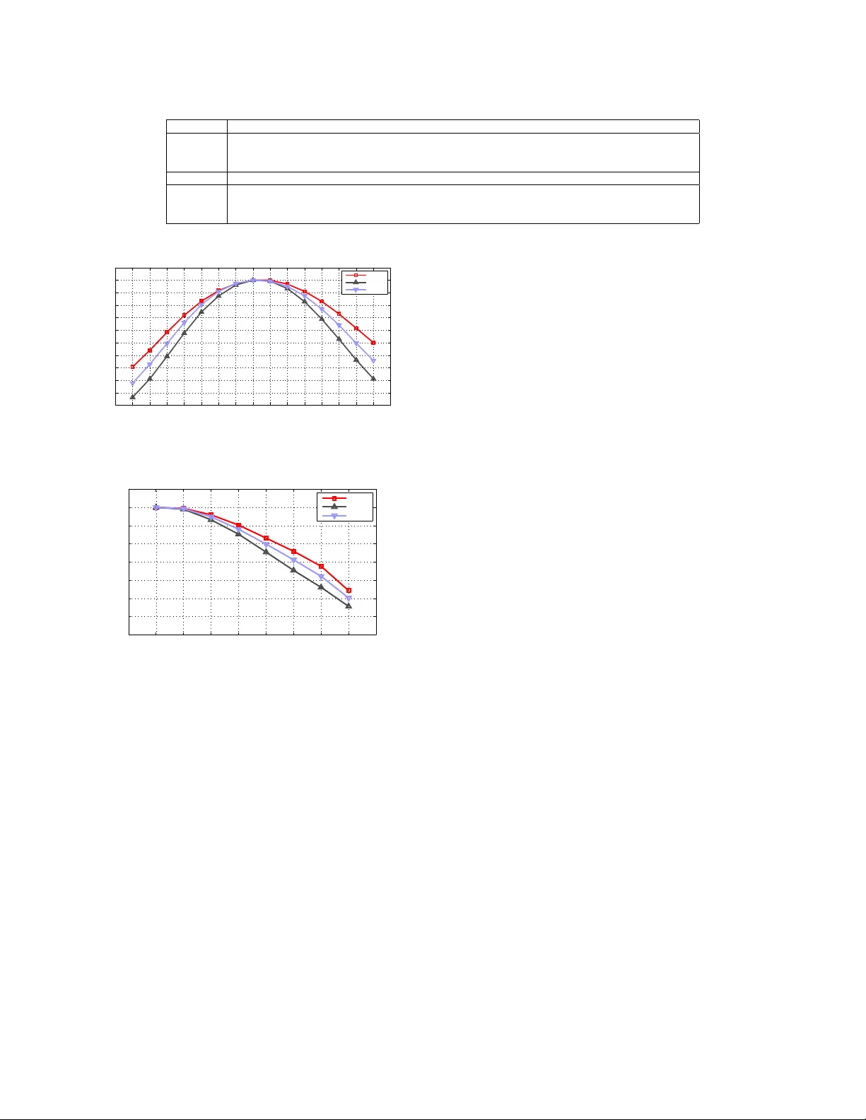
1 A Plug&Play P300 BCI Using Information Geometry Alexandre Barachant, Marco Congedo T eam V iBS (V ision and Brain Signal Processing), GIPSA-lab, CNRS, Grenoble Uni versities. France. Email: alexandre.barachant@gmail.com Abstract —This paper presents a new classification methods for Event Related Potentials (ERP) based on an Information geometry framework. Through a new estimation of covariance matrices, this work extend the use of Riemannian geometry , which was pre viously limited to SMR-based BCI, to the problem of classification of ERPs. As compared to the state-of-the-art, this new method increases perf ormance, r educes the number of data needed for the calibration and features good generalisation across sessions and subjects. This method is illustrated on data recorded with the P300-based game brain invaders . Finally , an online and adaptive implementation is described, where the BCI is initialized with generic parameters derived from a database and continiously adapt to the individual, allowing the user to play the game without any calibration while keeping a high accuracy . Index T erms —ERP , BCI, Information geometry I . I N T RO D U C T I O N So far we ha ve conceiv ed a Brain-Computer Interface (BCI) as a learning machine where the classifier is trained in a calibration phase preceding immediately the actual BCI use [1]. Depending on the BCI paradigm and on the efficienc y of the classifier , the calibration phase may last from a fe w to sev eral minutes. Regardless the duration, the very necessity of a calibration session reduces drastically the usability and appealing of a BCI. This is true both for clinically-oriented BCI, where the cognitive skills of patients are often limited and are wasted in the calibration phase, and for healthy users where the plug&play operation is nowadays considered as a minimum requirement for any consumer interfaces and devices. Besides the essential considerations from the user perspectiv e, it appears evident that training the BCI at the beginning of each session and discarding the calibration data at the end is a very inef ficient way to proceed. The problem we pose here is: can we design a ”plug&play” BCI? Of course, such a goal does not imply that the BCI is not calibrated. What we want to achie ve is that the calibration is completely hidden to the user . One possible solution is to initialize the classification algorithm with generic parameters deriv ed from previous sessions and/or pre vious users and then to adapt continuously these parameters during the e xperiment in order to reach optimality for the current user in the current session. In order to do so our BCI must possess two key properties, namely: 1) good across-subject generalization and acr oss-session generalization , so as to yield appropriate accuracy (albeit sub-optimal) at the beginning of each session and ev en for the very first session of a BCI naiv e user . 2) fast conver gence toward the optimal parameters, that is, the adaptation should be efficient and robust (the adaptation is useless if it is effecti ve only at the end of the session). The two properties above are not trivial. On one hand, the methods inv olving spatial filtering enjoy fast conv ergence, but show a bad generalisation since the subspace projection is very specific to each subject and session. On the other hand, the methods working directly with low lev el, high dimensional space or features selected space sho w good generalization b ut require a lot of data to avoid o ver-fitting and therefore do not fulfil the property of fast conv ergence. W e have solved this problem before by working in the nativ e space of covariance matrices and using Riemannian geometry [2]. So far this framew ork was limited to BCIs based on motor imagery and SSVEP since the regular co- variance matrix estimation does not take into account the temporal structure of the signals, which is critical for ERP detection. Here we allow the use of our Riemannian geometry framew ork for ERP-based BCI by introducing a new smart way for b uilding covariance matrices. W e sho w experimentally that our new initialization/adaption BCI framew ork (based on Riemannian geometry) enjoys both properties 1) and 2). In addition, our method is rigorous, elegant, conceptually simple and computationally efficient. As a by-product the implementation is easier, more stable and compatible with the time constraints of a system operating on-line. Finally , thanks to the advance here presented we are able to propose a univ ersal framew ork for calibration-less BCIs, that is, the very same signal processing chain can be no w applied with minor modifications to any currently existing types of BCI. This paper is or ganized as follo ws. Section II introduce the metric, based on information geometry , that we are using in this work. Section III presents the classification algorithm and the new covariance matrix estimation method dedicated to the classification of ERPs. The method is illustrated on the P300 ERP . Results on three datasets are shown in section IV and compared to the state-of-the-art methods. Finally , we will conclude and discuss in section V. Related work: Over the past years, several attempt to design ”plug&play” BCI hav e been made. In [3], a pure machine- learning solution has been used for this purpose. For each user in a database, a complete classification chain (band-pass filtering, CSP spatial filtering, LDA classifier) is trained and optimized. Then, for a ne w user , all these classifiers are applied and the results are combined (different solutions are proposed) 2 in order to build a single classification result. In [4], [5], an unsupervised adaptation of a generic classifier is proposed to deal with inter-session and inter-subject variability in the context of the P300 speller . The proposed solution makes the use of the P300 constraints and language model to adapt a bayesian classifier and unsure the con vergence tow ard the optimal classifier . This solution is for now the most con vincing approach for the P300 speller . I I . A D I S TA N C E F O R T H E M U L T I V A R I A T E N O R M A L M O D E L A. Motivation Our goal is to use a method enjoying both properties of fast adaptation and generalisation across subjects and sessions in order to build an efficient adaptiv e classification chain. As we will see, none of the state-of-the-art methods fulfils these requirement, therefore we have to design a ne w classification algorithm. In essence, a classification algorithm works by comparing data to each other or to a prototype of the dif ferent classes. The notion of comparison implies the ability to measure dissimilarity between the data, i.e., the definition of a metric. Obviously , the accuracy of the classification is related to the ability of the metric to measure difference between classes for the problem at hand. The definition of the appropriate metric is not trivial and should be accomplished according to the intrinsic nature of the data. This problem is usually bypassed by the feature extraction process, which projects the raw data in a feature space where a well known metric (Euclidean distance, Mahalanobis distance, etc) is effecti ve. When the feature e xtraction is not able to complete the task, the metric could be embedded within the classification function by using a kernel trick, as in the Support V ector Machine (SVM) classifier . Nevertheless, the problem of choosing the kernel is not obvious and is generally solved by trials and errors, that is, by benchmarking se veral predefined kernel through a cross-validation procedure. Ho wev er proceeding this way one loose generalization [1]. The recent BCI systems follow these approaches, by using a subspace separation [6] procedure and a selection of relev ant dimensions [7] before applying the classifier on the extracted features. In these approaches, the weakness of the chain is the subspace separation process, which rely on several assumptions that are more or less fulfilled, depending on the number of classes and the quality of the data. In addition, the subspace separation gi ves solutions that are not generalisable between session and subjects. T o overcome these dif ficulties, the linear subspace separation could be embedded in the classifier by working directly on the cov ariance matrices [8] and using a SVM kernel to classify them [9]. Again, the choice of the kernel and its parameters is done heuristically which is incompatible with adaptiv e implementations. In this context, the definition of a metric adapted to the nature of EEG signals seems to be particularly useful. W ith such a metric, a very simple distance-based classifier can be used, allo wing ef ficient adaptiv e implementations, reducing the amount of data needed for calibration (no cross-v alidation or feature selection) and offering better generalization between subjects and sessions (no source separation or any other spatial filtering). B. An Information geometry metric Thanks to information geometry we are able to define a metric enjoying the sought properties. The information geometry is a field of information theory where the probability distributions are taken as point of a Riemannian manifold. This field has been popularised by S. Amari who has widely contributed to establish the theoretical background [10]. Infor - mation geometry has today reached its maturity and find an increasing number of practical applications, such as radar im- age processing [11], diffusion tensor imaging [12] and image and video processing [13]. The strength of the information geometry is to giv e a natural choice for an information- based metric according to the probability distribution fam- ily: the F isher Information [10]. Therefore, each probability distribution belongs to a Riemannian manifold with a well established metric leading to the definition of a distance between probability distributions. In this work, EEG signals are assumed to follow a mul- tiv ariate normal distrib ution with a zero mean (this is the case for EEG signals that are high-pass filtered), which is a common assumption [14]. More specifically , it has been shown that EEG signal are block stationary and can be purposefully modelled by second order statistics [15]. Let us denote by X ∈ R C × N an EEG trial 1 , recorded over C electrodes and N time samples. W e assume that this trial follow a multiv ariate normal model with zero mean and with a covariance matrix Σ ∈ R C × C , i.e. X ∼ N ( 0 , Σ ) (1) The application of information geometry to the multiv ariate model with zero mean provides us with a metric that can be used to compare directly covariance matrices of EEG segments. C. Distance Let us denote two EEG trials X 1 ∼ N ( 0 , Σ 1 ) and X 2 ∼ N ( 0 , Σ 2 ) . Their Riemannian distance according to information geometry is gi ven by [11] δ R ( Σ 1 , Σ 2 ) = k log  Σ − 1 / 2 1 Σ 2 Σ − 1 / 2 1  k F = " C X c =1 log 2 λ c # 1 / 2 , (2) where λ c , c = 1 . . . C are the real eigenv alues of Σ − 1 / 2 1 Σ 2 Σ − 1 / 2 1 and C the number of electrodes. Note that this distance is also called Affine-in variant [16] when it is obtained through the algebraic properties of the spaces of symmetric positiv e definite matrices rather than through the information geometry work-flo w . This distance has two im- portant properties of in variance. First, the distance is in variant by inv ersion, i.e., δ R ( Σ 1 , Σ 2 ) = δ R ( Σ − 1 1 , Σ − 1 2 ) . (3) 1 An epoch of EEG signal we want to classify . 3 Second, the distance is in variant by congruent transforma- tion, meaning that for any in vertible matrix V ∈ G l ( C ) we hav e δ R ( Σ 1 , Σ 2 ) = δ R ( V T Σ 1 V , V T Σ 2 V ) . (4) This latter property has numerous consequences on EEG signal. The most remarkable can be formulated as it follo ws: Any linear operation on the EEG signals that can be modelled by a C × C invertible matrix V has no effect on the Riemannian distance. Such a class of transformations include rescaling and nor- malization of the signals, electrodes permutations, whitening, spatial filtering or source separation, etc. In essence, manipu- lating cov ariance matrices with Eq.(2) is equiv alent to working in the optimal source space of dimension C . D. Geometric mean The Riemannian geometric mean of I cov ariance matrices (denoted by G ( . ) ), also called Fr ´ echet mean, is defined as the matrix minimizing the sum of the squared Riemannian distances [17], i.e., G ( Σ 1 , . . . , Σ I ) = arg min Σ ∈ P ( n ) I X i =1 δ 2 R ( Σ , Σ i ) . (5) There is no closed form expression for this mean, howe ver a gradient descent in the manifold can be used in order to find the solution [17]. A matlab implementation is provided in a Matlab toolbox 2 . Note that the geometric mean inherits the properties of in variance from the distance. E. Geodesic The geodesic is defined as the shortest curve between two points (in this work, covariance matrices) of the manifold [17]. The geodesic according to the Riemannian metric is given by Γ ( Σ 1 , Σ 2 , t ) = Σ 1 2 1  Σ − 1 2 1 Σ 2 Σ − 1 2 1  t Σ 1 2 1 , (6) with t ∈ [0 : 1] a scalar . Note that the geometric mean of two points is equal to the geodesic at t = 0 . 5 [18], i.e., G ( Σ 1 , Σ 2 ) = Γ ( Σ 1 , Σ 2 , 0 . 5) (7) Moreov er, the geodesic could be seen as a geometric in- terpolation between the two cov ariance matrices Σ 1 and Σ 2 . Its Euclidean equi valent is the well known linear interpolation (1 − t ) Σ 1 + t Σ 2 . I I I . M E T H O D A. Classification of covariance matrices Using the metric defined by the information geometry we are now able to efficiently compare EEG trials using only their cov ariance matrices. The direct classification of co variance matrices has pro ved very useful for single trial classification in the context of SMR- based BCI [2], [19], [9] and more generally in ev ery EEG application where the rele vant features are based on the spatial 2 http://github .com/alexandrebarachant/cov ariancetoolbox patterns of the signal. A similar approach, working on the power spectral density rather than the cov ariance matrix, has been developed for sleep state detection [20], [21]. According to the property of in variance of the distance, the Riemannian metric allows to bypass the source separation step by exploiting directly the spatial information contained in the cov ariance matrix. While the state-of-the-arts methods rely on the classification of the log-v ariances in the source space, the Riemannian metric giv es access to the same information in the sensor space, leading to a better generalization of the trained classifier . The Minimum Distance to Mean (MDM) algorithm is one of the simplest classification algorithm based on distance com- parison. Used with the Riemannian distance, it is a powerful and efficient way to build a an online BCI system [22]. Giv en a training set of EEG trials X i ∼ N ( 0 , Σ i ) and the corresponding labels y i ∈ { 1 : N c } , the classifier training consist in the estimation of a mean co variance matrix for each of the N c classes, ¯ Σ K = G ( Σ i | y i = K ) , (8) where K ∈ [1 : N c ] is the class label and G ( . ) is the Rieman- nian geometric mean defined in section II-D. In essence, the geometric mean represents the expected distribution that will follows a trial belonging to class K . Then, the classification of a ne w trial X ∼ N ( 0 , Σ ) of an unknown class y is simply achieved by looking at the minimun distance to each mean, ˆ y = arg min K δ R ( ¯ Σ K , Σ ) . (9) Such a classifier defines a set of vorono ¨ ı cells in the manifold. Alternativ ely , for binary classification problems, the difference of the two distances could be used as a linear classification score. The algorithm is extremely simple since it in volve only a mean estimation and a distance computation for each class. The full algorithm is giv en in Algorithm 1. Algorithm 1 Minimum Distance to Riemannian Mean Input: a set of trials X i of N c different known classes and the corresponding labels y i ∈ { 1 : K } . Input: X an EEG trial of unknown class. Output: ˆ y the estimated class of test trial X . 1: Compute SCMs of X i to obtain Σ i . 2: Compute SCM of X to obtain Σ . 3: for K = 1 to N c do 4: ¯ Σ K = G ( Σ i | y i = K ) , Riemannian geometric mean (5). 5: end for 6: ˆ y = arg min K δ R ( ¯ Σ K , Σ ) , Riemannian distance (2). 7: retur n ˆ y B. Classification of covariance matrices in P300-based BCI The above procedure is not suitable for classification of ERPs, where the discriminant information is giv en by the wa veform of the potential rather than the spatial distribution of its variance. Indeed, the covariance matrix estimation does not take into account the time structure of the signal, and therefore using only the cov ariance matrix for the classification leads to the loss of the information carried by the temporal structure of the ERP . 4 More generally , the prior knowledge of a reference signal, i.e., the expected wav eform of the signal due to a physiological process (P300, ErrP , etc.) or induced by a stimulation pattern (SSEP), are rarely taken into account in the signal processing chain. Our contribution stems from the definition of a specific way of b uilding cov ariance matrices for ERP data embedding both the spatial and temporal structural information. This new defi- nition, making use of a reference signal, allows the purposeful application of Riemannian geometry for ERP data. Let us define P1 ∈ R C × N the prototyped ERP response, obtained, for example, by averaging several single trial responses of one class, usually the tar get class, such as P1 = 1 |I | X i ∈I X i . (10) where I is the ensemble of indexes of the trial belonging to the target class. For each trial X i ∈ R C × N , we build a super trial ˜ X i ∈ R 2 C × N by concatenating P1 and X i : ˜ X i =  P1 X i  . (11) These super trials are used to b uild the co variance matrices on which the classification will be based. The cov ariance matrices are estimated using the Sample Cov ariance Matrix (SCM) estimator: ˜ Σ i = 1 N − 1 ˜ X i ˜ X T i . (12) These cov ariances matrices can be decomposed in three different blocks : Σ P 1 the cov ariance matrix of P1 , Σ i the cov ariance matrix of X i and C P 1 ,X i the cross-cov ariance matrix (non-symmetric) between P1 and X i , that is, ˜ Σ i =  Σ P 1 C T P 1 ,X i C P 1 ,X i Σ i  . (13) Σ P 1 is the same for all the trials. This block is not useful for the discrimination between the different classes. Σ i is the cov ariance matrix of the trial i . As explained pre viously , this block is not sufficient to achieve a high classification accuracy . Howe ver , it contains information that can be used in the classification process. The cross-cov ariance matrix C P 1 ,X i contains the major part of the useful information. If the trial contains an ERP in phase with Σ P 1 , the cross-co variance will be high for the corresponding channels. In other cases (absence of ERP or non phase locked ERP), the cross-covariance will be close to zero, leading to a particular cov ariance structure that can be e xploited by the classification algorithm. Note that the property of in variance of the metric allo ws to use a reduced version of P1 after a source separation and a selection of relev ant sources if desired. Using this ne w estimation, the MDM algorithm can be applied in the exact same manner, using ˜ X i Eq.(11) instead of X i in Algorithm 1. In the case of ERP , only two classes are used, target for trials containing an ERP and non-target for the others, leading to the estimation of two mean cov ariance matrices, denoted ¯ Σ T and ¯ Σ ¯ T , respecti vely . For this binary classification task, the classification score for each trial is gi ven by the difference of the Riemannian distance to each class, i.e., s = δ R ( ¯ Σ ¯ T , Σ ) − δ R ( ¯ Σ T , Σ ) . (14) C. An adaptive implementation W e employ here a simple adaptation scheme. When new data from the current subject is av ailable, the two subject- specific intra-class mean cov ariance matrices ¯ Σ s T and ¯ Σ s ¯ T are estimated and combined with the tw o generic ones (computed on a database) ¯ Σ g T and ¯ Σ g ¯ T using a geodesic interpolation: ¯ Σ K = Γ ( ¯ Σ g K , ¯ Σ s K , α ) , (15) where Γ is the geodesic from ¯ Σ g K to ¯ Σ s K giv en in Eq.(6), with K denoting T ( ¯ T ) for the target (non-target) class and with α ∈ [0 : 1] a parameter settings the strength of the adaptation ev olving from 0 at the be ginning of the session to 1 at the end of the session. This combination is the Riemannian equiv alent to (1 − α ) ¯ Σ g K + α ¯ Σ s K in the euclidean space. The combined matrices are then used for the classification in replacement of the standard mean cov ariances matrices in Algorithm 1. A similar approach has been presented for the adaptation of spatial filters in [23]. The adaptation is supervised, i.e., the classes of the trials hav e to be known. This not a limitation in applications where the tar get is chosen by the interface itself and not by the user . For other ERP-based BCI such as a P300 speller , adaptation will be somehow slower since only past symbols (that the user has confirmed) can be used. Howe ver , an unsupervised adaptation is also possible using clustering of cov ariance matrices in Riemannian space. Preliminary results (not shown here) show that this approach is equiv alent to the supervised one. I V . R E S U L T S A. Material The presented method is illustrated through the detection of P300 ev oked potentials on three datasets. These datasets are recorded using the P300-based game Brain In vaders [24]. Brain inv aders is inspired from the famous vintage game Space in vaders. The goal is to destroy a target alien in a grid of non-target alien using the classical P300 paradigm. After each repetition, i.e., flash of the 6 rows and 6 columns, the most probable alien is destroyed according to the single trial classification scores of the 12 flashes. If the target alien is destroyed, the game switch to the next level. If not, a new repetition begins and its classification scores will be av eraged with the scores of the previous repetitions. Therefore, the goal of the game is to complete all le vels in a minimum number of repetitions. B. Prepr ocessing and State-of-the-art methods Motiv ate the Choice Reference methods For each method and dataset, signals are bandpass filtered by a 5th order butterworth filter between 1 and 20 Hz. Filtered signal are then downsampled to 128 Hz and segmented in 5 epochs of 1s starting at the time of the flash. T wo state of the art methods hav e been implemented for comparison with the proposed method. The first is named XDA WN and is com- posed by a spatial filtering using the xD A WN method [25] and a re gularized LD A [26] for classification. After the estimation of spatial filters, the two best spatial filters are applied on the epochs. The spatially filtered epoch are then downsampled by a factor four and the time sample are aggregated to build a feature vector of size 32 × 2 = 64 . These feature vectors are then classified using a regularized LDA. The second method is name SWLDA and is composed by a single classification stage using a stepwise LD A [26]. First the signals were downsampled by a factor four and aggregated to b uild a feature vector of size 32 × C . These feature vectors are classified using a stepwise LD A [26]. The stepwise LD A performs a stepwise model selection before applying a regular linear discriminant analysis, reducing the number of features used for classification. The MDM method is directly applied on the epochs of signal, with no other preprocessing besides the frequency band-pass filtering and do wnsampling. C. Dataset I Dataset I was recorded in laboratory conditions using 10 silver/silv er-chloride electrodes (T7-Cz-T8-P7-P3-PZ-P4-P8- O1-O2) and a Nexus amplifier (TMSi, The Netherlands). The signal was sampled at 512 Hz. 23 subjects participated to this experiment for one session composed of a calibration phase of 10 minutes and a test phase of 10 minutes. This dataset is used to ev aluate offline performances of the methods in the canonical training-test paradigm. 1) Canonical performances: In this section, performances will be ev aluated using the classical training-test paradigm. Algorithms are calibrated on the data recorded during the training phase, and applied on the data recorded during the test phase (online). The Area Under R OC Curve (A UC), estimated on the classification scores Eq.(14) will be used as criterion to ev aluate the effecti veness of the trained classifier . T able I reports these A UC for the 23 subjects and the three ev aluated methods. The MDM method offers the best performances among the three methods. Even if the mean improv ement is small, the difference is significant (t-test for paired sample; MDM vs. XD A WN : t (22) = 4 . 001 , p = 0 . 0006 ; MDM vs. SWLD A : t (22) = 4 . 482 , p = 0 . 0002 ). On the contrary , there is no significant difference between the two reference methods (t- test for paired sample; XD A WN vs. SWLD A : t (22) = 1 . 172 , p = 0 . 26 ). W e can also note that the improvement is higher for subjects with low performances ( 0 . 75 < AU C < 0 . 9 , e.g., subjects 4, 9, 18, 19 and 21). Overall, the proposed method exhibits an excellent classification accuracy , despite its simplicity . 2) Effect of the size of the training set on performances: The size of the calibration data-set is usually a critical pa- rameter influencing dramatically the results. T o e valuate this effect on the MDM algorithm, we calibrate the algorithm using an increasing number of trials from the training set. Figure 1 shows the results of this test. 1 4 7 10 13 16 19 22 25 28 31 34 37 40 43 46 49 52 55 58 61 0.5 0.55 0.6 0.65 0.7 0.75 0.8 0.85 0.9 Number of repetition used for calibration Mean AUC MDM SWLDA XDAWN Figure 1. Performances of the three methods as a function of the number of trials used for the calibration. 1 repetition = 12 trials, 2 target and 10 non-target. As expected, the three methods con ver ge to their optimal value. The SWLD A is the method with the slo west con vergence; due to the high dimension of the feature space, the model selection needs a lot of data to reach efficiency . On the contrary , the XD A WN method reduces the feature space and therefore needs less data for calibration. Finally , the MDM method shows the best results and the fastest con vergence. Thus, the MDM method could be used either to achie ve higher performance or to reduce the time spent in the calibration phases, while keeping the same accuracy . As example, in order to obtain a mean A UC of 0.85, only 13 repetitions are needed for the MDM, 22 for XD A WN and 52 for the SWLD A. 3) Effect of the latency and jitter of the evoked potential on performances: The correct detection of the ev oked potentials relies on the fact that the evok ed response is perfectly syn- chronized with the stimulus, i.e., it occurs always at the same time after each stimulus. In practice, a variable delay (jitter) and a fixed delay (latency) is observed, due to technical factors ( Hardware / Software Trigger , screen rendering) as well as physiological factors (fatigue, stress, mental workload). The dif ferent classification methods are more or less rob ust to theses nuisances. These factors are simulated by adding artificial delays on the test data. T o test the ef fect of latency , the triggers of the test data are shifted with a fixed delay from -55ms to 55 ms. Results are reported in Figure 2. Performances are normalized with the A UC obtained with a zero delay and subjects 7 and 8 where removed; because of their lo w performances, close to the chance level, delays have almost no effects on theses two subjects. In Figure 3, the effect of the jitter is studied by adding a random delay for each triggers of the test data. This delay is drawn from a normal distribution with a zero mean and standard deviation from 0ms to 55ms. In both cases, the loss of performance induced by the delay is less important for the MDM than for the other methods. Because of the model selection, the SWLDA method is the 6 T able I AU C O N T E ST DAT A F O R T H E 23 S U B JE C T S O F T H E D A TA S ET I F O R T H E 3 E V A L UA T E D ME T H O DS . Methdod 1 2 3 4 5 6 7 8 9 10 11 12 MDM 0.89 0.93 0.97 0.88 0.95 0.90 0.65 0.65 0.87 0.97 0.94 0.86 SWLD A 0.84 0.90 0.97 0.81 0.90 0.91 0.55 0.69 0.79 0.96 0.89 0.84 XD A WN 0.89 0.90 0.97 0.85 0.91 0.90 0.56 0.66 0.79 0.95 0.83 0.86 13 14 15 16 17 18 19 20 21 22 23 mean (std) MDM 0.88 0.92 0.93 0.91 0.98 0.84 0.78 0.97 0.90 0.95 0.96 0.89 (0.09) SWLD A 0.87 0.91 0.91 0.90 0.95 0.76 0.73 0.95 0.84 0.93 0.97 0.86 (0.10) XD A WN 0.88 0.90 0.93 0.91 0.96 0.77 0.74 0.96 0.84 0.92 0.96 0.86 (0.10) −54.7 −46.9 −39.1 −31.2 −23.4 −15.6 −7.8 0.0 7.8 15.6 23.4 31.2 39.1 46.9 54.7 50 55 60 65 70 75 80 85 90 95 100 105 Delay in ms Percentage of no−delay AUC MDM SWLDA XDAWN Figure 2. Effect of the latency on the performances. 0.0 7.8 15.6 23.4 31.2 39.1 46.9 54.7 65 70 75 80 85 90 95 100 105 Std of delay in ms Percentage of no delay AUC MDM SWLDA XDAWN Figure 3. Effect of the jitter on the performances. most sensitive method to the delay . 4) Effect of P 1 on performances: The estimation of the super-co variance matrices explained in section III-B is super- vised and requires the a verage P300 matrix P1 . Therefore, it is interesting to see how sensitive the method is regarding to the parameter P1 . T o do so, we apply the same test described in section IV -C1, but replacing the subject specific estimation of P1 by the grand average P300 ev oked response estimated on other users or using data from another experiment (data from Dataset II). Results sho w that there is no statistical difference when a cross-subject P1 (CSP1) or a cross-experiment P1 (CEP1) is used compared to the subject specific P1 ( t-test for paired samples, P1 vs. CSP1 : t (22) = − 0 . 776 , p = 0 . 45 ; P1 vs. CEP1 : t (22) = 0 . 175 , p = 0 . 86 ). These results, particularly meaningful, demonstrate that the critical parameters of the algorithm are the intra-class mean cov ariance matrices rather than the prototyped ev oked responses. Interestingly , it is possible to use an ev oked response from another experiment without loss of performances, e ven if the electrode montage is dif ferent. This effect comes from the property of in variance by congruent projection of the Riemannian metric. Thus, the matrix P1 could be estimated in the sources space, with a different electrodes montage or electrodes permutation, and any kind of scaling factor could be applied. W e will come back to this interesting property in the discussion section. 5) Cr oss-subjects performances: Results from the pre vious section show that the supervised estimation of the cov ariance matrices can be done in an unsupervised way by using the P300 av erage response from other subjects without loss of performances. Ho wever , calibration data are still required for the estimation of the intra-classe mean cov ariance matrices. Nev ertheless, it is possible to use data from other subjects to estimate the mean co variance matrices as well. T able II report performances of the different methods for each subject when calibration is done using data from other subjects, according to a leav e-one-out procedure. In these circumstances, the MDM method offers the best performances with a mean A UC of 0.82. On the other hand, the XDA WN method displays a really poor performance. This is not surprising since the estimation of spatial filters are known to be very subject specific. Even if the performances of SWLD A are significantly lower than those obtained with the MDM ( t (22) = 1 . 76 , p = 0 . 04 ), reg arding to its subject spe- cific performances, the SWLDA of fers a good generalization across subjects. W e can also notice that for subject 7 the cross subject cali- bration of fers better results as compared to the subject specific calibration. This is generally the case when the calibration data are of low quality , pointing to a general merit of generic initialization. D. Dataset II For a BCI game such brain in vaders where the session are generally short (less than 10 minutes) it is not acceptable for the user to do a calibration phase before each game. The second dataset has been recorded to study the gener- alization of parameters across different sessions. Dataset II was recorded in realistic conditions using 16 golden-plated dry electrodes (Fp1-Fp2-F5-AFz-F6-T7-Cz-T8-P7-P3-Pz-P4- P8-O1-Oz-O2) and a USBamp amplifier (Guger T echnologies, Graz, Austria). The signal was sampled at 512 Hz. 4 subjects participated to this experiment and made 6 sessions recorded on different days. Each session was composed of a single test phase, without any calibration phase, using cross subjects 7 T able II AU C O N T E ST DAT A F O R T H E 23 S U B JE C T S O F T H E D A TA S ET I I N A S U B JE C T SP E C I FIC A N D C R OS S S UB J E C T ( C S ) M A N N ER . 1 2 3 4 5 6 7 8 9 10 11 12 MDM 0.89 0.93 0.96 0.88 0.95 0.90 0.65 0.65 0.87 0.97 0.94 0.86 CS MDM 0.71 0.92 0.82 0.80 0.90 0.72 0.73 0.64 0.87 0.80 0.88 0.86 SWLD A 0.84 0.90 0.96 0.81 0.90 0.91 0.55 0.69 0.79 0.96 0.89 0.84 CS SWLD A 0.71 0.84 0.93 0.72 0.82 0.77 0.76 0.67 0.74 0.86 0.79 0.75 XD A WN 0.89 0.90 0.96 0.85 0.91 0.90 0.56 0.66 0.79 0.95 0.83 0.86 CS XD A WN 0.60 0.86 0.86 0.77 0.73 0.79 0.75 0.64 0.67 0.77 0.76 0.70 13 14 15 16 17 18 19 20 21 22 23 mean (std) MDM 0.88 0.92 0.93 0.91 0.98 0.84 0.78 0.97 0.90 0.95 0.96 0.89 (0.09) CS MDM 0.89 0.77 0.91 0.89 0.95 0.72 0.77 0.84 0.76 0.85 0.84 0.82 (0.08) SWLD A 0.87 0.91 0.91 0.90 0.95 0.76 0.73 0.95 0.84 0.93 0.97 0.86 (0.10) CS SWLD A 0.86 0.72 0.86 0.86 0.94 0.67 0.79 0.87 0.74 0.84 0.83 0.80 (0.08) XD A WN 0.88 0.90 0.93 0.91 0.96 0.77 0.74 0.96 0.84 0.92 0.96 0.86 (0.10) CS XD A WN 0.88 0.64 0.83 0.85 0.89 0.64 0.77 0.86 0.73 0.72 0.74 0.76 (0.09) parameters for the first session and cross sessions parameters for the next sessions. Offline results are reported in Fig. 4. W e study first the cr oss-subject performance by initializing the classifier with all the data of the other subjects. Results of number of sessions ”0” represent the grand average A UC across all subjects and all sessions. Then we study the cr oss- session performance by initializing the classifier of each subject with an increasing number of his/her own sessions and testing on the remaining sessions. For any n number of sessions used for calibration (x-axis), results represent the grand average A UC obtained on all combinations of the remaining 6 − n sessions for all subjects. 0 1 2 3 4 5 0.7 0.75 0.8 0.85 0.9 Number of sessions used for calibration Mean AUC Mean AUC in function of the number of calibration sessions Cross−session Cross− subject MDM XDAWN SWLDA Figure 4. Individual performances accross session for the 4 subjects when an increasing number of sessions are used for calibration. First, the cross subject classification gives a similar trend as the results obtained on the first dataset. Here the MDM clearly outperform the reference methods. W e could also notice that despite we hav e only four subjects in the database, the cross subject performances are surprisingly good. Second, the MDM methods sho ws better cross sessions performances as compared to SWLD A and XDA WN. In this experiment, the sessions are short and contain a small number of trial. For this reason, the SWLD A has dif ficulty to achiev e a high A UC when the number of training sessions is small. On the av erage, the same performance could be obtained with only two sessions for the MDM and fi ve sessions for the SWLD A. E. Dataset III Results on dataset I and II demonstrate the good properties of adaptation and generalization of the proposed method. These properties are necessary to obtain an ef ficient adaptiv e use of the algorithm. Dataset III was recorded in real-life conditions, using the same electrode montage and amplifier as the Dataset II. Sessions were recorded during a liv e demonstration at the g.tec W orkshop, held in our laboratory in Grenoble on March 5th 2013. Five subjects external to our laboratory played the Brain In vaders game for the first time in their life in a noisy en vironment. They made a single session without calibration using the online adaptiv e implementation of the MDM de- scribed in section III-C. Figure 5 reports online results. The performance is reported in terms of number of repetitions needed to destroy the target alien for each of nine lev els of the game. The adapti ve MDM, implemented in p ython within the open source software OpenV ibe [27], was initialized with parameters extracted using the data from the dataset II. As 1 2 3 4 5 6 7 8 9 0.5 1 1.5 2 2.5 3 3.5 4 Level of Brain Invaders Number of repetitions Figure 5. Mean and sd of the number of repetitions needed to destroy the target. expected, the adaptation improves the performance (t-test for slope < 0 : t (7) = − 3 . 82 , p = 0 . 007 ). On average players needed 2.5 repetitions at the beginning of the game session and only 1.5 for the last le vel. In addition, the variability decreases, and typically for the last two lev els less than two repetitions only suffice to destroy the target. This is a very good result as compared to the state-of-the-art. 8 V . C O N C L U S I O N W e hav e proposed a new classification method for ERP- based BCI that increases performance, reduces the number of data needed for the calibration and features good generalisa- tion across sessions and subjects. In addition, this new method prov es more robust against fixed and variable delays on the trigger signals as compared to state-of-the-art methods. An adaptiv e implementation has been deployed on our real-life experiments allowing the user to play without any calibra- tion (plug&play) while keeping a high accuracy . The Brain In vaders and the OpenV iBE scenarios we use are open-source and available for download 3 . V I . D I S C U S S I O N In this work a very simple classifier (MDM) has been used in order to facilitate the adaptiv e implementation. In our previous works on motor imagery more sophisticated classification algorithms has been developed, leading to higher performances as compared to the MDM. In [28], a geodesic filtering was applied before the MDM in order to improv e class separability . In [19], a SVM-kernel dedicated to cov ariance matrices was defined and another way of dealing with inter- session v ariability was proposed. These methods gi ve promis- ing results but show less stability in a cross-subject context. In future works we will in vestigate whether more complex classification methods based on information geometry can be used in an adapti ve context. W ith the ne w definition of cov ariances matrices proposed in this article the Riemannian geometry frame work can now be applied on all the three main BCI paradigms (SMR, ERP , SSEP) with only minor modifications. A single imple- mentation of the classification method can be used for the different paradigms, which is very conv enient in terms of software development and maintenance. Besides the Rieman- nian frameworks, the new proposed estimation of cov ariance matrix for ERP brings permeability between states-of-the-art methods since the wide majority of signal processing alorithms for SMR-based BCIs rely on the manipulation of cov ariance matrices. For example, the well known CSP spatial filtering and all its v ariations can now be applied for ERPs. Finally , the property of inv ariance of the metric giv es great freedom in the choice of the prototyped ERP matrix P1 . This matrix could be drawn by hand, or generated with a wavelets basis, allo wing, for example, to adapt the system to dif ferent sampling frequency . Howe ver , this approach shows some limitations when the number of channels increase. If the number of channel is greater than the number of time sample in the trial, the cov ariance matrix is ill-conditioned and the computation of the Riemannian distance becomes impossible. In this context, a regularized estimate of the covariance matrix must be used, or if it is possible, a higher sampling frequency . In addition, if the number of channel is too big ( > 64 ), the estimation of the mean covariance matrices might not conv erge. In this case, consider to use a smaller number of channel or apply a 3 http://code.google.com/p/open vibe-gipsa-extensions/ subspace reduction (PCA) to decrease the dimensionality of the problem. R E F E R E N C E S [1] F . Lotte, M. Congedo, A. L ´ ecuyer , F . Lamarche, B. Arnaldi et al. , “ A revie w of classification algorithms for eeg-based brain–computer interfaces, ” Journal of neural engineering , vol. 4, 2007. [2] A. Barachant, S. Bonnet, M. Congedo, and C. Jutten, “Multiclass Brain-Computer interface classification by riemannian geometry , ” IEEE T ransactions on Biomedical Engineering , vol. 59, no. 4, pp. 920–928, 2012. [3] S. Fazli, C. Grozea, M. Danoczy , B. Blankertz, F . Popescu, and K.-r . M ¨ uller , “Subject independent eeg-based bci decoding, ” in Advances in Neural Information Processing Systems , 2009, pp. 513–521. [4] P .-J. Kindermans, D. V erstraeten, and B. Schrauwen, “ A bayesian model for exploiting application constraints to enable unsupervised training of a p300-based bci, ” PloS one , vol. 7, no. 4, p. e33758, 2012. [5] P .-J. Kindermans, H. V erschore, D. V erstraeten, and B. Schrauwen, “ A p300 bci for the masses: Prior information enables instant unsupervised spelling, ” in Advances in Neural Information Pr ocessing Systems 25 , 2012, pp. 719–727. [6] C. Gouy-Pailler, M. Congedo, C. Brunner , C. Jutten, and G. Pfurtscheller , “Nonstationary brain source separation for multiclass motor imagery , ” Biomedical Engineering, IEEE T ransactions on , vol. 57, no. 2, pp. 469–478, 2010. [7] M. Grosse-W entrup and M. Buss, “Multiclass common spatial patterns and information theoretic feature e xtraction, ” Biomedical Engineering, IEEE T ransactions on , vol. 55, no. 8, pp. 1991–2000, 2008. [8] J. Farquhar , “ A linear feature space for simultaneous learning of spatio- spectral filters in BCI, ” Neural Networks , vol. 22, no. 9, pp. 1278–1285, 2009. [9] B. Reuderink, J. Farquhar, M. Poel, and A. Nijholt, “ A subject- independent brain-computer interface based on smoothed, second-order baselining, ” in Engineering in Medicine and Biology Society ,EMBC, 2011 Annual International Confer ence of the IEEE , 2011, pp. 4600 – 4604. [10] S. Amari, H. Nagaoka, and D. Harada, Methods of information geometry . American Mathematical Society , 2000. [11] F . Barbaresco, “Innovati ve tools for radar signal processing based on cartan’ s geometry of SPD matrices & information geometry , ” in IEEE Radar Confer ence , 2008. [12] P . T . Fletcher and S. Joshi, “Principal geodesic analysis on symmetric spaces: Statistics of diffusion tensors, ” in Computer V ision and Mathe- matical Methods in Medical and Biomedical Image Analysis , 2004, pp. 87–98. [13] O. T uzel, F . Porikli, and P . Meer , “Pedestrian detection via classification on Riemannian manifolds, ” vol. 30, no. 10, pp. 1713–1727, 2008. [14] M. Congedo, C. Gouy-Pailler , and C. Jutten, “On the blind source separation of human electroencephalogram by approximate joint diag- onalization of second order statistics, ” Clinical Neurophysiolo gy , vol. 119, no. 12, pp. 2677–2686, 2008. [15] P . Comon and C. Jutten, Handbook of Blind Source Separation: Inde- pendent component analysis and applications . Academic press, 2010. [16] V . Arsigny , P . Fillard, X. Pennec, and N. A yache, “Geometric means in a novel vector space structure on symmetric positive-definite matrices, ” SIAM journal on matrix analysis and applications , vol. 29, no. 1, pp. 328–347, 2007. [17] X. Pennec, P . Fillard, and N. A yache, “ A riemannian framew ork for tensor computing, ” International Journal of Computer V ision , vol. 66, no. 1, pp. 41–66, 2006. [18] M. Moakher, “ A differential geometric approach to the geometric mean of symmetric Positi ve-Definite matrices, ” SIAM J. Matrix Anal. Appl. , vol. 26, no. 3, pp. 735–747, 2005. [19] A. Barachant, S. Bonnet, M. Congedo, and C. Jutten, “Classification of cov ariance matrices using a Riemannian-based kernel for bci applica- tions, ” Neurocomputing , vol. 112, pp. 172–178, 2013. [20] Y . Li, K. M. W ong, and H. DeBruin, “Eeg signal classification based on a riemannian distance measure, ” in Science and T echnology for Humanity (TIC-STH), 2009 IEEE T oronto International Confer ence . IEEE, 2009, pp. 268–273. [21] Y . Li, K. W ong, and H. Bruin, “Electroencephalogram signals classifi- cation for sleepstate decision-a riemannian geometry approach, ” Signal Pr ocessing, IET , vol. 6, no. 4, pp. 288–299, 2012. 9 [22] A. Barachant, S. Bonnet, M. Congedo, C. Jutten et al. , “ A brain-switch using riemannian geometry , ” in Proceedings of the 5th International BCI Confer ence 2011 , 2011, pp. 64–67. [23] F . Lotte and C. Guan, “Regularizing common spatial patterns to improv e bci designs: unified theory and ne w algorithms, ” Biomedical Engineer- ing, IEEE Tr ansactions on , vol. 58, no. 2, pp. 355–362, 2011. [24] M. Congedo, M. Goyat, N. T arrin, G. Ionescu, L. V arnet, B. Riv et, R. Phlypo, N. Jrad, M. Acquadro, and C. Jutten, “”Brain In vaders”: a prototype of an open-source P300- based video game working with the OpenV iBE platform, ” in Pr oceedings of the 5th International Brain- Computer Interface Conference 2011 , Graz, Autriche, 2011, pp. 280– 283. [25] B. Rivet, A. Souloumiac, V . Attina, and G. Gibert, “xdawn algorithm to enhance ev oked potentials: application to brain–computer interface, ” Biomedical Engineering, IEEE Tr ansactions on , vol. 56, no. 8, pp. 2035– 2043, 2009. [26] D. J. Krusienski, E. W . Sellers, F . Cabestaing, S. Bayoudh, D. J. Mcfar - land, T . M. V aughan, and J. R. W olpaw , “A comparison of classification techniques for the P300 speller, ” Journal of Neural Engineering , vol. 3, no. 4, pp. 299–305, Oct. 2006. [27] Y . Renard, F . Lotte, G. Gibert, M. Congedo, E. Maby , V . Delannoy , O. Bertrand, and A. L ´ ecuyer , “Open vibe: an open-source software platform to design, test, and use brain-computer interfaces in real and virtual environments, ” Presence: teleoperator s and virtual en vironments , vol. 19, no. 1, pp. 35–53, 2010. [28] A. Barachant, S. Bonnet, M. Congedo, and C. Jutten, “Riemannian geometry applied to bci classification, ” in Latent V ariable Analysis and Signal Separation . Springer , 2010, pp. 629–636. Alexandre Barachant was born in Chateauroux, France, in 1985. In 2012, he reciev ed the Ph.D. degree in signal processing from the Grenoble Uni- versity , Grenoble, France. He has worked at CEA- LETI during his Ph.D. on the topic of brain computer interfaces. He his actually a post-doc fellow at the Centre National de la Recherche Scientique (CNRS) in the GIPSA Laboratory , Grenoble, France. His current research interest include statistical signal processing, Riemannian geometry and classification of neurophysiological recordings with applications to brain computer interfaces. Marco Congedo obtained the Ph.D. degree in Bio- logical Psychology with a minor in Statistics from the University of T ennessee, Knoxville, in 2003. From 2003 to 2006 he has been a post-doc fel- low at the French National Institute for Research in Informatics and Control (INRIA) and at France T elecom R&D, in France. Since 2007 Dr . Congedo is a Research Scientist at the ”Centre National de la Recherche Scientifique” (CNRS) in the GIPSA Laboratory , Grenoble, France. Dr . Congedo has been the recipient of sev eral awards, scholarships and re- search grants. He is interested in basic human electroencephalography (EEG) and magnetoencephalography (MEG), real-time neuroimaging (neurofeedback and brain-computer interface) and multiv ariate statistical tools useful for EEG and MEG such as in verse solutions, blind source separation and Riemannian geometry . Currently he is Academic Editor of journal PLoS ONE.