Boosted Markov Networks for Activity Recognition

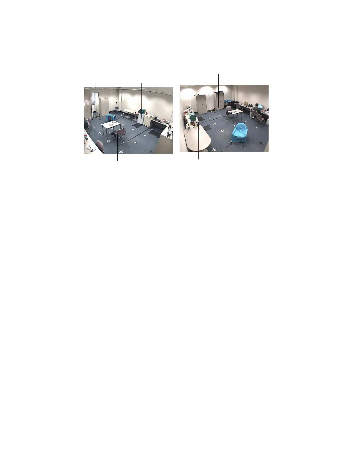
Bo osted Mark o v Net w orks for Activit y Recognition # T ran The T ruy en 1 , Hung Hai Bui 2 , Sv etha V enk atesh 3 Dep artment of Computing, Curtin University of T e chnolo gy GPO Box U 1987, Perth, W A, A ustr alia. 1 , 3 { tr antt2,svetha } @cs.curtin.e du.au, 2 bui@ai.sri.c om Abstract W e explore a framew ork called bo osted Marko v netw orks to com bine the learning capacit y of bo osting and the ric h modeling seman tics of Marko v netw orks and ap- plying the framework for video-based activity recognition. Importantly , w e extend the framework to incorp orate hidden v ariables. W e show ho w the framework can b e applied for b oth model learning and feature selection. W e demonstrate that b oosted Mark ov net works with hidden v ariables perform comparably with the standard max- im um lik eliho od estimation. How ev er, our framework is able to learn sparse models, and therefore can provide computational savings when the learned mo dels are used for classification. 1 In tro duction Recognising human activities using sensors is currently a ma jor c hallenge in research. T ypically , the information extracted directly from sensors is either not discriminative enough or is to o noisy to infer activities occurring in the scene. Human activities are complex and ev olve dynamically ov er time. T emp oral probabilistic mo dels suc h as hid- den Marko v mo dels (HMMs) and dynamic Bay esian netw orks (DBNs) hav e b een the dominan t mo dels used to solv e the problem [1, 4, 19]. Ho wev er, these mo dels make a strong assumption in the generativ e pro cess by which the data is generated in the mo del. This makes the representation of complex sensor data very difficult, and possibly results in large mo dels. Mark ov net works (MNs) (also kno wn as Mark ov random fields) offer an alternativ e approac h, esp ecially in form of conditional random fields (CRFs) [10]. In CRFs, the ob- serv ation is not modelled, and so we hav e the freedom to incorp orate ov erlapping features, m ultiple sensor fusion, and long-range dep endencies into the mo del. The discriminativ e nature and the underlying graphical structure of the MNs mak e it esp ecially suitable to the problem of human activity recognition. Bo osting is a general framework to gradually improv e the performance of the weak learner (which can b e just slightly b etter than a random guess). A p opular version called AdaBo ost [6, 14, 15] forces the weak learner to focus more on hard-to-learn examples from the examples seen so far. The final strong learner is the weigh ted sum of all weak learners added to this ensemble in each iteration. Most of the work so far with b o osting in volv es only unstructured output, except for a few occasions, such as the work in [2, 5, 18]. 1 W e are motiv ated to use bo osting for parameter estimation of Mark ov netw orks (which w e call b oosted Marko v netw orks (BMNs)), as recent results ha ve sho wn the close rela- tionship b et ween b oosting and the maximum likelihoo d estimation (MLE) [8, 11]. F ur- thermore, we use the inherent capacit y of b oosting for feature selection integrated with learning. W e are motiv ated b y studies that the t ypical log-linear mo dels imposed on Mark ov netw orks can easily b e ov erfitted with little data and many irrelev ant features, but can b e o vercome b y the use of explicit feature selection, either indep enden tly or in tegrated with learning (e.g. see [13]). Previous work [2, 5, 18] hav e explored the BMNs sho wing promising results. The BMNs integrate the discriminative learning p o w er of b oosting and the rich semantics of the graphical mo del of Mark ov netw orks. In this pap er, w e further explore alternativ e metho ds for this approac h. T o handle hidden v ariables as in the standard MLE, w e extend the work b y Altun et al. [2]. This is a v arian t of the multiclass bo osting algorithm called AdaBo ost.MR [6, 15]. W e also suggest an appro ximation pro cedure for the case of intractable output structures. The prop osed framework is demonstrated through our exp erimen ts in which b o osting can provide a comparable p erformance to MLE. Ho wev er, since our framework uses sparse features it has the potential to provide computational sa vings during recognition. The no velt y of the pap er is t wo-fold: a) W e presen t the first w ork in applying bo osting for activit y recognition, and b) w e deriv e a b oosting pro cedure for structured mo dels with missing v ariables and use a parameter up date based on quadratic appro ximation instead of lo ose upper b ounds as in [2] to sp eed up the learning. The organisation of the pap er is as follows. The next section reviews related work. Section 3 presents the concept of bo osted Marko v netw orks (BMNs) detailing how b oost- ing is emplo yed to learn parameters of Mark ov net works. Section 4 goes into the details of efficien t computation for tree-structured and general netw orks. W e then describ e our exp erimen ts and results in applying the mo del to video-based human activity recognition in an indo or en vironment. The last section discusses any remaining issues. 2 Related w ork Our w ork is closely related to that in [5], where b oosting is applied to learn parameters of the CRFs using gradien t trees [7]. The ob jectiv e function is the log-likelihoo d in the standard MLE setting, but the training is based on fitting regression trees in a stage-wise fashion. The final decision function is in the form of a linear combination of regression trees. [5] employs functional gradients for the log-loss in a manner similar to LogitBo ost [8], whilst we use the original gradients of the exp onen tial loss of AdaBoost [6, 14, 15]. Th us [5] learns the model b y maximising the likelihoo d of the data, while w e are motiv ated b y minimising the errors in the data directly . Moreo ver, [5] indirectly solves the structured mo del learning problem of MLE by con verting the problem to a standard unstructured learning problem with regression trees. In contrast, w e solve the original structured learning problem directly without the structured-unstructured con version. In addition, the pap er in [5] do es not incorporate hidden v ariables as our work do es. Another work, [18], integrates the message passing algorithm of b elief propagation (BP) with a v ariant of LogitBoost [8]. Instead of using the p er-net work loss as in [5], the authors of [18] emplo y the p er-lab el loss (e.g. see [3] for details of the tw o losses), that is they use the marginal probabilities. Similar to [5], [18] also conv erts the structured learning problem in to a more con ven tional unstructured learning problem. The algorithm th us alternates b etw een a message passing round to up date the lo cal p er-lab el log-losses, and a b oosting round to up date the parameters. Ho wev er, as the BP is in tegrated in the algorithm, it is not made clear on how to apply different inference tec hniques when the BP fails to conv erge in general net works. It is also unclear on how to extend the method to deal with hidden v ariables. There hav e b een a num b er of attempts to exploit the learning p o wer of b oosting applied to structured mo dels other than Marko v netw orks, such as dynamic Ba yesian net works (DBNs) [9], Ba yesian net work classifier [21], and HMMs [20]. 3 Bo osted Mark o v net w orks 3.1 Mark o v net w orks W e are in terested in learning a structured model in whic h inference procedures can b e p erformed. A typical inference task is deco ding, e.g. to find the most probable lab el set (configuration) y ∗ for the netw ork given an observ ation x y ∗ = arg max y p ( y | x ). F or a single no de netw ork, this is often called the classification problem. F or a net work of N no des, the num b er of configurations is exp onen tially large. W e assume the conditional exp onen tial distribution (a.k.a. log-linear mo del) p ( y | x ) = 1 Z ( x ) exp( F ( x, y )) (1) where Z ( x ) = P y exp( F ( x, y )) is the normalisation factor, and F ( x, y ) = P k λ k f k ( x, y ). { f k } are features or weak hypotheses in b oosting literature. This conditional mo del is kno wn as the conditional random fields (CRFs) [10]. The deco ding reduces to y ∗ = arg max y F ( x, y ). Often, in Marko v net works the follo wing decomp osition is used f k ( x, y ) = X c f k ( x, y c ) (2) where c is the index of the clique defined by the structure of the netw ork. This decomp o- sition is essential to obtain a factorised distribution, whic h is vital for efficient inference in tree-like structures using dynamic programming. Denote by y = ( v , h ) the visible and hidden v ariables (which are represented b y no des in the netw ork). Given n i.i.d observ ations { x i } n i =1 , maximum likelihoo d learning in MNs minimises the log-loss L log = − X i log p ( v i | x i ) = X i log 1 p ( v i | x i ) (3) 3.2 Exp onen tial loss for incomplete data W e view the activit y lab eling and segmen tation problems as classification where the n um- b er of distinct classes is exp onen tially large, i.e. | Y | N , where | Y | is the size of lab el set, and N is the n umber of no des in the Mark ov netw ork. F ollo wing the dev elopment by Altun et al. [2], we define a new exp e cte d r anking loss [15] to incorp orate hidden v ariables as follows L rank = X i X h p ( h | v i , x i ) X v 6 = v i δ [∆ F ( x i , v, h ) > 0] (4) where ∆ F ( x i , v, h ) = F ( x i , v, h ) − F ( x i , v i , h ), and δ [ z ] is the indicator function of whether the predicate z is true. This rank loss captures the expectation of moments in which the classification is wrong b ecause if it is true, then max v F ( x i , v, h ) = F ( x i , v i , h ) implying F ( x i , v, h ) < F ( x i , v i , h ) ∀ v 6 = v i . Ho wev er, it is muc h more conv enient to deal with a smo oth conv ex loss and th us w e form ulate an upp er b ound of the rank loss, e.g. the exponential loss L exp = X i X h p ( h | v i , x i ) X v exp(∆ F ( x i , v, h )) (5) It is straightforw ard to chec k that (5) is indeed an upp er b ound of (4). It can b e seen that (4) includes the loss prop osed in [2] as a sp ecial case when all v ariables are observed, i.e. y = v . It is essentially an adapted v ersion of AdaBo ost.MR prop osed in [15]. A difficulty with this form ulation is that we do not know the true conditional distri- bution p ( h | v i , x i ). First, we approximate it by the learned distribution at the previous iteration. Thus, the conditional distribution is up dated along the wa y , starting from some guessed distribution, for example, a uniform distribution. Second, we assume the log-linear mo del as in (1), leading to X v exp(∆ F ( x i , v, h )) = P v exp( F ( x i , v, h )) exp( F ( x i , v i , h )) = 1 p ( v i | h, x i ) whic h can b e fed into (5) to obtain L exp = X i X h p ( h | v i , x i ) p ( v i | h, x i ) = X i 1 p ( v i | x i ) (6) W e can notice the similarity b et ween the exp onential loss in (6) and the log-loss in (3) as log(.) is a monotonically increasing function. The difference is the exponential scale used in (6) with resp ect to features { f k } compared to the linear scale in (3). 3.3 Bo osting-based learning The typical bo osting pro cess has man y rounds, each of which selects the b est weak h y- p othesis and finds the weigh t for this hypothesis to minimise the loss. T ranslated in our con text, the b oosting-based learning searches for the b est feature f j and its coefficient to add to the ensemble F t +1 = F t + α t f j so that the loss in (5) is minimised. ( α t , j ) = arg min α,k L exp ( t, α, k ) , where (7) L exp ( t, α, k ) = X i E h | v i ,x i ,t [ X v exp(∆ F i,t + α ∆ f i k )] where E h | v i ,x i ,t [ z ( h )] = P h p ( h | v i , x i , t ) z ( h ); F i,t and f i k are shorthands for F t ( x i , v, h ) and f k ( x i , v, h ), resp ectiv ely . Note that this is just an approximation to (5) because w e fix the conditional distribution p ( h | v i , x i , t ) obtained from the previous iteration. How ever, this still makes sense since the learning is incremen tal, and thus the estimated distribution will get closer to the true distribution along the wa y . Indeed, this captures the essence of b o osting: during each round, the w eak learner selects the w eak hypothesis that b est minimises the following loss o ver the w eighted data distribution (see [15]) ( α t , j ) = arg min α,k X i X v ,h D ( i, v , h, t ) exp( α ∆ f i k ) (8) where the w eighted data distribution D ( i, v, h, t ) = p ( h | v i , x i , t ) exp(∆ F i,t ) / Z ( i, t ) with Z ( i, t ) being the normalising constant. Since the data distribution do es not contain α , (8) is identical to (7) up to a constant. 3.4 Beam search It should b e noted that b oosting is a v ery generic framework to b o ost the p erformance of the weak learner. Th us we can build more complex and stronger weak learners b y using some ensemble of features and then later fit them in to the b o osting framew ork. Ho wev er, here we stic k to simple w eak learners, which are features, to mak e the algorithm compatible with the MLE. W e can select a num b er of top features and asso ciated co efficien ts that minimise the loss in (8) instead of just one feature. This is essen tially a beam searc h with specified b eam size S . 3.5 Regularisation W e employ the l 2 regularisation term to make it consistent with the p opular Gaussian prior used in conjunction with the MLE of Marko v netw orks. It also maintains the con vexit y of the original loss. The regularised loss b ecomes L reg = L non − reg + X k λ 2 k 2 σ 2 k (9) where L non − reg is either L log for MLE in (3) or L exp for b o osting in (5). Note that the regularisation term for b oosting do es not ha ve the Bay esian interpretation as in the MLE setting but is simply a constraint to prev ent the parameters from gro wing to o large, i.e. the model fits the training data to o well, whic h is clearly sub-optimal for noisy and unrepresen tative data. The effect of regularisation can b e numerically v ery different for the tw o losses, so w e cannot exp ect the same σ for both MLE and b oosting. 4 Efficien t computation Straigh tforward implemen tation of the optimisation in (7) or (8) by sequentially and iterativ ely searc hing for the b est features and parameters can be impractical if the num b er of features is large. This is partly b ecause the ob jective function, although it can b e tractable to compute using dynamic programming in tree-like structures, is still exp ensiv e. W e propose an efficient approximation which requires only a few vectors and an one-step ev aluation. The idea is to exploit the conv exity of the loss function by appro ximating it with a con vex quadratic function using second-order T aylor’s expansion. The change due to the up date is appro ximated as ∆ J ( α , k ) ≈ dJ ( α , k ) dα     α =0 α + 1 2 d 2 J ( α , k ) dα 2     α =0 α 2 (10) where J ( α, k ) is a shorthand for L ( t, α, k ). The selection pro cedure b ecomes ( α t , j ) = arg min α,k J ( α , k ) = arg min α,k ∆ J ( α , k ). The optimisation ov er α has an analytical solution α t = − J 0 /J 00 . Once the feature has b een selected, the algorithm can pro ceed by applying an addi- tional line searc h step to find the b est coefficient as α t = arg min α L ( t, α, j ). One wa y to do is to rep eatedly apply the up date based on (10) until conv ergence. Up to now, w e hav e made an implicit assumption that all computation can b e car- ried out efficiently . How ever, this is not the case for general Marko v netw orks b ecause most quantities of interest inv olv e summation ov er an exp onen tially large num b er of net work configurations. Similar to [2], w e show that dynamic programming exists for tree-structured netw orks. How ev er, for general structures, appro ximate inference must b e used. There are three quan tities we need to compute: the distribution p ( v i | x i ) in (6), the first and second deriv ative of J in (10). F or the distribution, we hav e p ( v i | x i ) = P h p ( v i , h | x i ) = Z ( v i , i ) / Z ( i ) where Z ( v i , i ) = P h exp( P c F ( x i , v i c , h c )) and Z ( i ) = P y exp( P c F ( x i , y c )). Both of these partition functions are in the form of sum-pro duct, th us, they can be computed efficiently using a single pass through the tree-like structure. The first and second deriv atives of J are then J 0 | α =0 = X i E h | v i ,x i ,t [ X v exp(∆ F i,t )∆ f i k ] (11) J 00 | α =0 = X i E h | v i ,x i ,t [ X v exp(∆ F i,t )(∆ f i k ) 2 ] (12) Expanding (11) yields J 0 | α =0 = X i 1 p ( v i | x i , t ) X v ,h p ( v , h | x i , t )∆ f i k (13) Note that f i k has the additiv e form as in (2) so ∆ f k ( x i , y ) = P c ∆ f k ( x i , y c ). Thus (13) reduces to J 0 | α =0 = X i 1 p ( v i | x i , t ) X c X y c p ( y c | x i , t )∆ f k ( x i , y c ) (14) whic h no w con tains clique marginals and can be estimated efficiently for tree-like structure using a down ward and up ward sweep. F or general structures, lo opy b elief propagation can provide approximate estimates. Details of the pro cedure are omitted here due to space constraints. Ho wev er, the computation of (12) do es not enjo y the same efficiency b ecause the square function is not decomp osable. T o make it decomp osable, we emplo y Cauch y’s inequalit y to yield the upp er b ound of the change in (10) (∆ f k ( x i , y )) 2 = ( X c ∆ f k ( x i , y c )) 2 ≤ | C | X c ∆ f k ( x i , y c ) 2 where | C | is the num b er of cliques in the netw ork. The up date using α = − J 0 / ˜ J 00 , where ˜ J 00 is the upp er b ound of the second deriv ative J 00 , is rather conserv ative, so it is clear that a further line search is needed. Moreo ver, it should b e noted that the change in (10), due to the Newton up date, is ∆ ˜ J ( α , k ) = − 0 . 5( J 0 ) 2 / ˜ J 00 , where ∆ ˜ J is the upper bound of the c hange ∆ J due to Cauc hy’s inequalit y , so the weak learner selection using the optimal change do es not dep end on the scale of the second deriv ativ e b ound of ˜ J 00 . Thus the term | C | in Cauch y’s inequality ab o v e can b e replaced b y any con venien t constant. The complexit y of our b o osting algorithm is the same as that in the MLE of the Mark ov netw orks. This can b e verified easily b y taking the deriv ative of the log-loss in (3) and comparing it with the quantities required in our algorithm. 5 Exp erimen tal results W e restrict our attention to the linear-chain structure for efficien t computation b ecause it is sufficient to learn from the video data we capture. F or all the exp erimen ts rep orted here, we train the mo del using the MLE along with the limited memory quasi-Newton metho d (L-BFGS) and we use the prop osed b o osting scheme with the help of a line search, satisfying Amijo’s conditions. F or regularisation, the same σ is used for all features for simplicit y and is empirically selected. In the training data, only 50% of lab els are randomly giv en for eac h data slice in the sequence. F or the performance measure, we rep ort the per-lab el error and the av erage F 1-score ov er all distinct lab els. 5.1 Data and feature extraction In this pap er, we ev aluate our b oosting framework on video sensor data. How ever, the framew ork is applicable to different t yp e of sensors and is able to fuse different sen- sor information. The observ ational environmen t is a kitchen and dining ro om with t wo cameras moun ted to t wo opp osite ceiling corners (Figure 1). The observ ations are se- quences of noisy co ordinates of a person walking in the scene extracted from video using a background subtraction algorithm. The data was collected in our recent work [12], con- sisting of 90 video sequences spanning three scenarios: SHOR T MEAL, HA VE SNA CK and NORMAL MEAL. W e pick a slightly smaller num b er of sequences, of which we se- lect 42 sequences for training and another 44 sequences for testing. Unlik e [12], w e only build flat mo dels, thus separate mo dels for each scenario are learned and tested. The lab els are sequences of the ‘activities’ the p erson is p erforming, for example ‘going-fr om- do or-to-fridge’ . F or training, only partial lab el sets are given, lea ving a p ortion of the lab el missing. F or testing, the labels are not provided, and the lab els obtained from the deco ding task are compared against the ground-truth. It turns out that informativ e features are critical to the success of the mo dels. A t the same time, the features should b e as simple and intuitiv e as p ossible to reduce manual Dinning chair Door Fridge TV chair TV chair Stove Fridge Dinning chair Cupboard Figure 1: The environmen t and scene viewed from the tw o cameras. lab our. A t eac h time slice τ , we extract a vector of 5 elements from the observ ation sequence g ( x, τ ) = ( X , Y , u X , u Y , s = p u 2 X + u 2 Y ), which corresp ond to the ( X, Y ) co or- dinates, the X & Y v elo cities, and the sp eed, resp ectiv ely . These observ ation features are approximately normalised so that they are of comparable scale. 5.2 Effect of feature selection F ollowing previous b oosting applications (e.g.[16]), w e emplo y v ery simple decision rules: a w eak hypothesis (feature function) returns a real v alue if certain conditions on the training data p oin ts are met, and 0 otherwise. W e design three feature sets. The first set, called the activity-p ersistenc e , captures the fact that activities are in general p ersisten t. The set is divided into data-asso ciation features f l,m ( x, y τ ) = δ [ y τ = l ] g m ( x, τ ) (15) where m = 1 , .., 5, and lab el-label features f l,m ( x, y τ − 1 , y τ ) = δ [ y τ − 1 = y τ ] δ [ y τ = l ] (16) Th us the set has K = 5 | Y | + | Y | features, where | Y | is the size of the lab el set. The second feature set consists of tr ansition-fe atur es that are in tended to enco de the activit y transition nature as follo ws f l 1 ,l 2 ,m ( x, y τ − 1 , y τ ) = δ [ y τ − 1 = l 1] δ [ y τ = l 2] g m ( x, τ ) (17) Th us the size of the feature set is K = 5 | Y | 2 . The third set, called the c ontext set , is a generalisation of the second set. Observ ation- features no w incorp orate neigh b ouring observ ation p oin ts within a sliding window of width W g m ( x, τ ,  ) = g m ( x, τ +  ) (18) T able 1: P erformance on three data sets, activit y-p ersistence features. SM = SHOR T MEAL, HS = HA VE SNA CK , NM = NORMAL MEAL, Agthm = algorithm, itrs = n umber of iterations, ftrs = num b er of selected features, % ftrs = p ortion of selected features. Data SM SM HS HS NM NM Agthm MLE Bo ost MLE Bo ost MLE Bo ost σ ∞ ∞ ∞ ∞ ∞ ∞ error(%) 10.3 16.6 12.4 14.5 9.7 17.2 F1(%) 86.0 80.2 84.8 82.1 87.9 77.4 itrs 100 500 100 200 100 200 # ftrs 30 30 30 30 42 35 % ftrs 100 100 100 100 100 83.3 where  = − W l , .. 0 , ..W u with W l + W u + 1 = W . This is intended to capture the correlation of the current activity with the past and the future, or the temporal c ontext of the observ ations. The second feature set is a sp ecial case with W = 1. The num b er of features is a multiple of that of the second set, which is K = 5 W | Y | 2 . The b oosting studied in this section has the b eam size S = 1, i.e. eac h round picks only one feature to up date its weigh t. T ables 1, 2, 3 sho w the p erformance of the training algorithms on test data of all three scenarios (SHOR T MEAL, HA VE SNACK and NOR- MAL MEAL) for the three feature sets, resp ectiv ely . Note that the infinite regularisation factor σ means that there is no regularisation. In general, sequen tial b o osting app ears to b e slow er than the MLE b ecause it up dates only one parameter at a time. F or the activit y persistence features (T able 1), the feature set is v ery compact but informative enough so that the MLE attains a reasonably high p erformance. Due to this compactness, the feature selection capacity is almost eliminated, leading to p oorer results as compared with the MLE. Ho wev er, the situation changes radically for the activit y transition feature set (T able 2) and for the con text feature set (T able 3). When the observ ation con text is small, i.e. W = 1, b oosting consistently outp erforms the MLE whilst main taining only a partial subset of features ( < 50% of the original feature set). The feature selection capacity is demonstrated more clearly with the context-based feature set ( W = 11), where less than 9% of features are selected by bo osting for the SHOR T MEAL scenario, and less than 3% for the NORMAL MEAL scenario. The b oosting p erformance is still reasonable despite the fact that a very compact feature set is used. There is therefore a clear computational adv antage when the learned mo del is used for classification. 5.3 Learning the activit y-transition mo del W e demonstrate in this section that the activit y transition model can b e learned by b oth the MLE and bo osting. The transition feature sets studied previously do not separate the transitions from data, so the transition mo del may not b e correctly learned. W e design another feature set, which is the bridge b et ween the activity-persistence and the transition feature set. Similar to the activit y p ersistence set, the new set is divided into T able 2: P erformance on activity transition features Data SM SM HS HS NM NM Agthm MLE Bo ost MLE Bo ost MLE Bo ost σ ∞ ∞ ∞ ∞ ∞ ∞ error(%) 18.6 10.1 13.0 10.8 15.0 16.5 F1(%) 75.8 89.3 86.8 85.7 81.4 80.9 itrs 59 200 74 100 53 100 # ftrs 125 57 125 44 245 60 % ftrs 100 45.6 100 35.2 100 24.5 T able 3: P erformance on context features with window size W = 11 Data SM SM HS HS NM NM Agthm MLE Bo ost MLE Bo ost MLE Bo ost σ 2 2 ∞ ∞ ∞ ∞ error(%) 15.3 9.6 9.4 11.2 9.3 16.6 F1(%) 81.6 87.7 89.3 86.6 87.7 78.1 itrs 51 200 22 100 21 100 # ftrs 1375 115 1375 84 2695 80 % ftrs 100 8.36 100 6.1 100 3.0 data-asso ciation features, as in (15), and lab el-label features f l 1 ,l 2 ( y τ − 1 , y τ ) = δ [ y τ − 1 = l 1] δ [ y τ = l 2] (19) Th us the set has K = 5 | Y | + | Y | 2 features. Giv en the SHOR T MEAL data set, and the activity transition matrix in T able 4, the parameters corresp onding to the lab el-lab el features are given in T ables 5 and 6, as learned by b o osting and MLE, respectively . A t first sight, it may be tempting to select non-zero parameters and their asso ciated transition features, and hence the corresp onding transition mo del. How ever, as tran- sition features are non-negative (indicator functions), the mo del actually penalises the probabilities of an y configurations that activ ate negative parameters exp onen tially , since p ( y | x ) ∝ exp( λ k f k ( y τ − 1 , y τ )). Therefore, huge negativ e parameters practically corre- sp ond to improbable configurations. If we replace all non-negative parameters in T able 5 and 6 by 1, and the rest by 0, w e actually obtain the transition matrix in T able 4. The T able 4: Activit y transition matrix of SHOR T MEAL data set Activit y 1 2 3 4 11 1 1 1 0 0 0 2 0 1 1 0 1 3 0 0 1 1 0 4 0 0 0 1 0 11 0 0 0 0 1 T able 5: P arameter matrix of SHOR T MEAL data set learned by b oosting Activit y 1 2 3 4 11 1 1.8 0 -5904.9 -5904.9 0 2 -5904.9 3.6 0 -5904.9 0 3 -5904.9 -5904.9 2.425 0 -5904.9 4 -5904.9 -5904.9 -5904.9 2.4 -5904.9 11 -5904.9 -5904.9 -5904.9 -5904.9 2.175 T able 6: P arameter matrix of SHOR T MEAL data set learned by MLE Activit y 1 2 3 4 11 1 10.81 4.311 -5.7457 -5.3469 -1.8398 2 -2.2007 15.056 3.6388 -5.6644 0.41921 3 -5.3565 -2.3131 9.3656 1.6575 -2.3736 4 -5.4103 -4.556 -4.1142 7.1332 -5.2976 11 -3.17 -0.09001 -2.9518 -4.8741 8.9128 difference b etw een b oosting and MLE is that b oosting p enalises the improbable transi- tions muc h more sev erely , th us leading to muc h sharp er decisions with high confidence. Note that for this data set, b oosting learns a m uch more correct mo del than the MLE, with an error rate of 3.8% ( F 1 = 93.7%), in constrast to 15.6% ( F 1 = 79.5%) by the MLE without regularisation, and 11.8% ( F 1 = 85.0%) b y the MLE with σ = 5. 5.4 Effect of b eam size Recall that the b eam search describ ed in Section 3.4 allo ws the w eak h yp othesis to be an ensem ble of S features. When S = K , all the parameters are updated in parallel, so it is essen tially similar to the MLE, and th us no feature selection is p erformed. W e run a few exp erimen ts with different b eam sizes S , starting from 1, which is the main fo cus of this pap er, to the full parameter set K . As S increases, the n umber of selected features also increases. How ever, w e are quite inconclusive ab out the final p erformance. It seems that when S is large, the update is quite po or, leading to slow con vergence. This is probably b ecause the diagonal matrix resulting from the algorithm is not a go od approximation to the true Hessian used in Newton’s up dates. It suggests that there exists a go o d, but rather mo derate, b eam size that p erforms b est in terms of b oth the conv ergence rate and the final p erformance. An alternative is just to minimise the exp onen tial loss in (5) directly b y using any generic optimisation method (e.g. see [2, 3]). Ho wev er, this approach, although may b e fast to conv erge, loses the main idea b ehind b o osting, which is to re-weigh the data distribution on each round to fo cus more on hard-to-classify examples as in (8). These issues are left for future inv estigation. 6 Conclusions and F urther w ork W e hav e presented a scheme to exploit the discriminative learning p o wer of the bo ost- ing metho dology and the semantically rich structured mo del of Marko v net works and in tegrated them into a b oosted Mark ov net work framework whic h can handle missing v ariables. W e hav e demonstrated the p erformance of the newly proposed algorithm o ver the standard maximum-lik eliho od framework on video-based activity recognition tasks. Our preliminary results on structure learning using bo osting indicates promise. Moreo ver, the built-in capacity of feature selection by b o osting suggests an in teresting application area in small footprint devices with limited pro cessing pow er and batteries. W e plan to in vestigate ho w to select the optimal feature set online b y hand-held devices given the pro cessor, memory and battery status. Although empirically shown to b e successful in our exp erimen ts, the p erformance guaran tee of the framework is yet to b e prov en, p ossibly following the large margin ap- proac h as in [14, 17], or the asymptotic consistency in the statistics literature as with the MLE. In the application to sensor net works, w e intend to explore methods to incorp orate ric her sensory information into the w eak learners, and to build more expressive structures to mo del m ulti-level and hierarc hical activities. Ac kno wledgmen ts The Matlab co de of the limited memory quasi-Newton metho d (L-BFGS) to optimise the log-lik eliho o d of the CRFs is adapted from S. Ulbrich. References [1] J. K. Aggarwal, Q. Cai, “Human motion analysis: A review”, Computer Vision and Image Understanding , V ol. 73, No. 3, 1999, pp. 428-440. [2] Y. Altun, T. Hofmann, M. Johnson, “Discriminative Learning for Lab el Sequences via Bo osting”, A dvanc es in Neur al Information Pr o c essing Systems 15 , 2003, pp. 977-984. [3] Y. Altun, M. Johnson, T. Hofmann, “Inv estigating Loss F unctions and Optimization Metho ds for Discriminative Learning of Lab el Sequences”, In: Pr o c e e dings of the 2003 Confer enc e on Empiric al Metho ds in NLP , 2003. [4] H.H. Bui, S. V enk atesh, G. W est, “P olicy recognition in the abstract hidden Marko v mo del”, Journal of Articial Intel ligenc e R ese ar ch , V ol. 17, 2002, pp. 451-499. [5] T.G. Dietterich, A, Ashenfelter, Y. Bulatov, “T raining Conditional Random Fields via Gradient T ree Bo osting”, In: Pro c. 21 st International Conference on Machine Learning, 2004, Banff, Canada. [6] Y. F reund,R.E. Schapire, “A decision-theoretic generalization of on-line learning and an application to b o osting”, Journal of Computer and System Scienc es , V ol. 55, No. 1, 1997, pp. 119–139. [7] J. H. F riedman, “Greedy function appro ximation: a gradien t b oosting mac hine”, A nn. Statist , V ol. 29, No. 5, 2001, pp. 1189–1232. [8] J. F riedman, T. Hastie, R. Tibshirani, “Additive logistic regression: a statistical view of b oosting”, The Annals of Statistics , V ol. 28, No. 2, 2000, pp. 337–374. [9] A. Garg, V. Pa vlovic, J. Rehg, “Boosted Learning in Dynamic Bay esian Net works for Multimo dal Speaker Detection”, In: Pr o c. the IEEE , 2003. [10] J. Lafferty , A. McCallum, F. Pereira, “Conditional Random Fields: Probabilistic Mo dels for Segmen ting and Lab eling Sequence Data”, In: Pr o c. 18th International Conf. on Machine L e arning , 2001, pp. 282–289. [11] G. Lebanon, J. Laffert y , “Bo osting and Maximum Likelihoo d for Exp onential Mo d- els”, A dvanc es in Neur al Information Pr o c essing Systems 14 , 2002, pp. 447-454. [12] N. Nguyen, D. Phung, S. V enk atesh, H. H. Bui “Learning and detecting activities from mov ement tra jectories using the hierarc hical hidden Marko v mo dels”. In: Pr o c. CVPR , San Diego, CA, June 2005. [13] S. D. Pietra, V. D. Pietra, J. Laffert y , “Inducing F eatures of Random Field”, IEEE T r ansactions on Pattern Analysis and Machine Intel ligenc e , V ol. 19, No. 4, 1997, pp. 380–393. [14] R.E. Sc hapire, Y. F reund, P . Bartlett, W.S. Lee, “Bo osting the Margin: A New Explanation for the Effectiveness of V oting Metho ds”, The Annals of Statistics , V ol. 26, No. 5, 1998, pp. 1651-1686. [15] R.E. Sc hapire, Y. Singer, “Improv ed Boosting Using Confidence-rated Predictions”, Machine L e arning , V ol. 37, No. 3, 1999, pp. 297–336. [16] R.E. Schapire, Y. Singer, “Bo osT exter: A Bo osting-based System for T ext Catego- rization”, Machine L e arning , V ol. 39, No. 2/3, 2000, pp. 135-168. [17] B. T ask ar, C. Guestrin, D. Koller, “Max-Margin Marko v Netw orks”, A dvanc es in Neur al Information Pr o c essing Systems 16 , 2004. [18] A. T orralba, K.P . Murph y , W,T. F reeman, “Contextual Models for Ob ject Detection Using Bo osted Random Fields”, A dvanc es in Neur al Information Pr o c essing Systems 17 , 2005, pp. 1401-1408. [19] J. Y amato, J. Ohy a, K. Ishii, “Recognizing h uman action in time-sequen tial images using hidden Marko v models”, In: CVPR , 1992, pp. 379-385. [20] P . Yin, I. Ess a, J.M. Rehg, “Asymmetrically Bo osted HMM for Sp eech Reading”, In: Pr o c. CVPR , V ol. 2, No. 2, 2004, pp. 755-761. [21] Y. Jing, V. Pa vlovic, J.M. Rehg, “Efficient discriminative learning of Ba yesian net- w ork classifiers via bo osted augmented naive Ba yes”, In: Pr o c. ICML , 2005.