Consistent transformations of belief functions

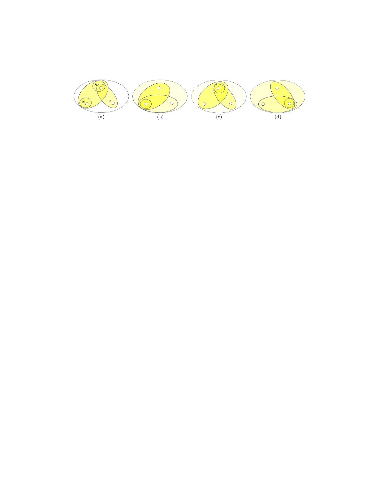
Consisten t transformations of b elief functions F abio Cuzzolin Dep artment of Computing and Communic ation T e chnolo gies Oxfor d Br o okes University Whe atley c ampus, Oxfor d OX33 1HX, Unite d Kingdom Abstract Consisten t b elief functions represen t collections of coherent or non-con tradictory pieces of evidence, but most of all they are the coun terparts of consisten t kno wledge bases in b elief calculus. The use of consistent transformations cs [ · ] in a reasoning pro cess to guaran tee coherence can therefore b e desir- able, and generalizes similar techniques in classical logics. T ransformations can b e obtained by minimizing an appropriate distance measure b et w een the original b elief function and the collection of consisten t ones. W e fo cus here on the case in which distances are measured using classical L p norms, in b oth the “mass space” and the “b elief space” representation of b elief functions. While mass consisten t approximations reassign the mass not fo cussed on a c hosen element of the frame either to the whole frame or to all sup ersets of the elemen t on an equal basis, approximations in the b elief space do distinguish these fo cal elements according to the “fo cussed consistent transformation” principle. The different appro ximations are in terpreted and compared, with the help of examples. Keywor ds: Theory of evidence, b elief logic, consistent belief functions, simplicial complex, L p norms, consisten t transformation. 1. In tro duction Belief functions (b.f.s) [1, 2] are complex ob jects, in which different and sometimes contradictory b o dies of evidence ma y co exist, as they mathemat- ically describ e the fusion of p ossibly conflicting exp ert opinions or measure- men ts. This is the case, for instance, of the p ose estimation problem in computer vision [ ? ]. There, image features do not necessary come from the ob ject of in terest, but ma y b e extracted from the bac kground: in such a case, Pr eprint submitte d to Information Scienc es Septemb er 1, 2021 the b elief functions inferred from those feature will conflict [ ? ]. Indeed, con- flict and com binability play a central role in the theory of evidence [3, 4, 5], and ha ve b een recen tly sub ject to no v el analyses [6, 7, 8]. Consistent know le dge b ases and b elief functions. Making decisions based on ob jects collecting p ossibly inconsisten t evidence, such as b elief functions, is therefore less than trivial. This is a well known problem in classical logics, where the application of inference rules to inconsisten t sets of assumptions or “kno wledge bases” may lead to incompatible conclusions, dep ending on the set of assumptions w e start our reasoning from [9]. A v ariety of approaches ha ve b een prop osed in this con text to solve the problem of inconsistent kno wl- edge bases, such as: fragmen ting the latter in to maximally consistent sub- sets; limiting the p o wer of the formalism; or, adopting non-classical seman tics [10, 11]. Ev en when a kno wledge base is formally inconsisten t, though, it may con tain p oten tially useful information. Paris [9] tackles the problem by not assuming eac h proposition in the kno wledge base as a fact, but b y attributing to it a certain degree of b elief in a probabilit y logic approach. This leads to something similar to a b elief function. Indeed, extensions of classical logics in which prop ositions are assigned b elief rather than truth v alues exist [33]. In this “b elief logic” framework, a b elief function can b e in terpreted as the analogous of a kno wledge base [12]. But then, what are the counterparts of consistent knowledge bases in the theory of evidence? T o answ er that w e need to sp ecify the notion of a b elief function “implying” a certain prop osition. As we sho w here, under a rather sensible definition of such an implication, the class of b elief functions which generalize consistent knowledge bases is uniquely determined as the set of b.f.s whose non-zero mass “fo cal elements” ha ve non-empt y in tersection. W e are therefore allo wed to call them c onsistent belief functions (cs.b.f.s). Consistent tr ansformation. Analogously to consistent knowledge bases, consisten t b.f.s are c haracterized b y n ull in ternal conflict. It ma y b e therefore b e desirable to transform a generic belief function to a consisten t one prior to making a decision, or pic king a course of action. A similar “transformation” problem has been widely studied in both the probabilistic [13, 14, 15, 16] and p ossibilistic [17, 18, 19] cases. A sensible approac h, in particular, consists of studying the geometry [20, 21] of the class of b.f.s of interest and pro jecting the original b elief function onto the corresponding geometric lo cus. Indeed, consistent transformations can be built b y solving a minimization 2 problem of the form: cs [ b ] = arg min cs ∈C S dist ( b, cs ) (1) where b is the original b elief function, dist an appropriate distance measure b et w een b elief functions, and C S denotes the collection of all consisten t b.f.s. By plugging in differen t distance functions in (1) w e get differen t consis- ten t transformations. Indeed, Jousselme et al [22] hav e recen tly conducted a v ery nice survey of the distance or similarit y measures so far introduced in b elief calculus, come out with an interesting classification, and prop osed a n umber of generalizations of kno wn measures. Man y of these measures could b e in principle employ ed to define indifferently consistent transformations or conditional b elief functions [23], or approximate b elief functions by necessit y or probabilit y measures. Other similarity measures b et ween b elief functions ha ve b een prop osed b y Shi et al [24], Jiang et al [25], and others [26, 27]. In this pap er w e fo cus on what happ ens when emplo ying classical L p norms in the approximation problem. The L ∞ norm, in particular, is closely related to consisten t and consonant b elief functions. The region of consisten t b.f.s can b e expressed as: C S = n b : max x ∈ Θ pl b ( x ) = 1 o , i.e., the set of b.f.s for which the L ∞ norm of the “plausibility distribution” or ”contour function” pl b ( x ) is equal to 1. In addition, cs.b.f.s relate to p ossibilit y distributions, and possibility measures P os are inherently associ- ated with L ∞ as P os ( A ) = max x ∈ A P os ( x ). In recen t times, L p norms hav e b een successfully employ ed in differen t problems such as probability [16] and p ossibilit y [28] transformation/appro ximation, or conditioning [23, 29]. As the author has prov en [30], geometrically , consisten t (as well as con- sonan t [31]) b elief functions live in a collection of simplices or “simplicial complex” C S . Eac h maximal simplex C S x of the consisten t complex is as- so ciated with asso ciated with an “ultrafilter” { A ⊇ { x }} , x ∈ Θ of focal elemen ts. A partial solution has therefore to be found separately for each maximal simplex of the consisten t complex: these partial solutions are later compared to determine the global approximation(s). In addition, geomet- ric appro ximation can b e p erformed in different Cartesian spaces. A b elief function can b e represented either by the vector ~ b = [ b ( A ) , ∅ ( A ( Θ] 0 of its b elief v alues, or the vector of its mass v alues ~ m b = [ m b ( A ) , ∅ ( A ( Θ] 0 . 3 W e call the set of vectors of the first kind b elief sp ac e B [21, 32], and the collection of v ectors of the second kind mass sp ac e M [23]. Contribution and outline. In this pap er, w e solv e the L p consisten t trans- formation problem in full generalit y in b oth the mass and the b elief space, and discuss the seman tics of the results. After briefly recalling a few basis notions of the theory of evidence, w e prov e that consisten t belief functions are the counterparts of consisten t kno wledge bases in belief logic (Section 2.2). As we inv estigate the transformation prob- lem in a geometric framew ork, w e briefly recall in Section 2.7 the geometry of the simplicial complex of consistent b elief functions, and explain ho w we need to solv e the approximation/transformation problem separately for eac h maximal simplex of this complex. W e then pro ceed to solv e the L 1 -, L 2 - and L ∞ -consisten t approximation problems in full generalit y , in b oth the mass (Section 3) and the b elief (Section 4) space represen tations. In Section 5 we compare and in terpret the outcomes of L p appro ximations in the tw o frame- w orks, with the help of the ternary example. W e conclude and discuss the natural prosecution of this line of researc h in Section 6. 2. Theory: consisten t approximations of b elief functions 2.1. Belief functions and b elief lo gic A b asic pr ob ability assignment (b.p.a.) on a finite set or fr ame of disc ern- ment Θ is a set function m b : 2 Θ → [0 , 1] on 2 Θ . = { A ⊆ Θ } s.t. m b ( ∅ ) = 0, P A ⊆ Θ m b ( A ) = 1. Subsets of Θ asso ciated with non-zero v alues of m b are called fo c al elements (f.e.), and their in tersection is called the c or e : C b . = \ A ⊆ Θ: m b ( A ) 6 =0 A. The b elief function (b.f.) b : 2 Θ → [0 , 1] asso ciated with a basic probability assignmen t m b on Θ is defined as: b ( A ) = X B ⊆ A m b ( B ). A dual mathematical represen tation of the evidence enco ded b y a belief func- tion b is the plausibility function (pl.f.) pl b : 2 Θ → [0 , 1], A 7→ pl b ( A ) where the plausibility v alue pl b ( A ) of an ev ent A is given b y pl b ( A ) . = 1 − b ( A c ) = P B ∩ A 6 = ∅ m b ( B ) and expresses the amount of evidence not against A . Generalizations of classical logic in which prop ositions are assigned prob- abilit y v alues hav e b een prop osed in the past. As b elief functions naturally 4 generalize probability measures, it is quite natural to define non-classical logic framew orks in which propositions are assigned b elief values , rather than probabilit y v alues. This approach has b een brought forward in particular b y Saffiotti [33], Haenni [12], and others. In prop ositional logic, prop ositions or formulas are either true or false, i.e., their truth v alue T is either 0 or 1 [34]. F ormally , an interpr etation or mo del of a form ula φ is a v aluation function mapping φ to the truth v alue “true” (1). Eac h formula can therefore b e asso ciated with the set of interpretations or mo dels under which its truth v alue is 1. If we define the frame of discern- men t of all the p ossible in terpretations, each form ula φ is asso ciated with the subset A ( φ ) of this frame whic h collects all its in terpretations. If the a v ailable evidence allo ws to define a b elief function on this frame of p ossible in terpretations, to eac h formula A ( φ ) ⊆ Θ is then naturally assigned a de- gree of b elief b ( A ( φ )) b et ween 0 and 1 [33, 12], measuring the total amount of evidence supp orting the prop osition “ φ is true”. 2.2. Semantics of c onsistent b elief functions In classical logic, a set Φ of formulas or “knowledge base” is said to b e c onsistent if and only if there do es not exist another formula φ suc h that the kno wledge base implies b oth the form ula and its negation: Φ ` φ , Φ ` ¬ φ . Hence, it is imp ossible to deriv e incompatible conclusions from the set of prop ositions whic h form a consisten t kno wledge base. This is crucial if w e w ant to derive univocal, non-con tradictory conclusions from a given b ody of evidence. A kno wledge base in prop ositional logic Φ = { φ : T ( φ ) = 1 } (where T ( φ ) denotes the truth v alue of prop osition φ ) corresp onds in belief logic [33] to a b elief function, i.e., a set of prop ositions together with their non-zero b elief v alues: b = { A ⊆ Θ : b ( A ) 6 = 0 } . T o determine what consistency amounts to in such a framework, w e need to formalize the notion of pr op osition implie d by a b elief function . One option is to decide that b ` B ⊆ Θ if B is implied b y all the prop ositions supp orted by b : b ` B ⇔ A ⊆ B ∀ A : b ( A ) 6 = 0 . (2) An alternative definition requires the prop osition B itself to receive non-zero supp ort b y the b elief function b : b ` B ⇔ b ( B ) 6 = 0 . (3) 5 Whatev er definition w e c ho ose for such implication relation, we can define the class of consistent belief functions as the set of b.f.s whic h cannot imply con tradictory prop ositions. Definition 1. A b elief function b is c onsistent if ther e exists no pr op osition A such that b oth A and its ne gation A c ar e implie d by b . When adopting the implication relation (2), it is easy to see that A ⊆ B ∀ A : b ( A ) 6 = 0 is equiv alent to T b ( A ) 6 =0 A ⊆ B . F urthermore, as each prop osition with non-zero b elief v alue must by definition con tain a fo cal elemen t C s.t. m b ( C ) 6 = 0, the in tersection of all non-zero b elief propositions reduces to that of all fo cal elemen ts of b , i.e., the core of b : \ b ( A ) 6 =0 A = \ ∃ C ⊆ A : m b ( C ) 6 =0 A = \ m b ( C ) 6 =0 C = C b . Indeed, no matter our definition of implication, the class of consistent b elief functions corresp onds to the set of b.f.s whose core is not empty . Definition 2. A b elief function is said consistent if its c or e is non-empty. W e can prov e that, under either definition (2) or definition (3) of the impli- cation b ` B , Definitions 1 and 2 are equiv alen t. Theorem 1. A b elief function b : 2 Θ → [0 , 1] has non-empty c or e if and only if ther e do not exist two c omplementary pr op ositions A, A c ⊆ Θ which ar e b oth implie d by b in the sense (2). Pr o of. A prop osition A is implied (2) by b iff C b ⊆ A . Accordingly , in order for b oth A and A c to b e implied b y b we w ould need C b = ∅ .  Theorem 2. A b elief function b : 2 Θ → [0 , 1] has non-empty c or e if and only if ther e do not exist two c omplementary pr op ositions A, A c ⊆ Θ which b oth enjoy non-zer o supp ort fr om b , b ( A ) 6 = 0 , b ( A c ) 6 = 0 (i.e., they ar e implie d by b in the sense (3)). Pr o of. By Definition 1, in order for a subset (or prop osition, in a prop ositional logic interpretation) A ⊆ Θ to ha ve non-zero b elief v alue it has to contain the core of b : A ⊇ C b . In order to hav e b oth b ( A ) 6 = 0, b ( A c ) 6 = 0 we need b oth to contain the core, but in that case A ∩ A c ⊇ C b 6 = ∅ which is absurd as A ∩ A c = ∅ .  6 2.3. A chieving c onsistency in b elief lo gic: c onsistent appr oximation Belief functions are complex ob jects, in which different and sometimes con tradictory b o dies of evidence co exist, as they ma y result from the fusion of p ossibly conflicting exp ert opinions and/or measuremen ts. It is reason- able to conjecture that taking b elief functions at face v alue ma y lead in some situations to incorrect/inappropriate decisions. A v ariet y of approac hes ha ve b een prop osed in the con text of classical log- ics to solve the analogous problem with inconsisten t kno wledge bases: we men tioned some of them in the introduction [10, 11]. P aris’ approac h [9] is particularly interesting as it tackles the problem b y attributing to eac h prop osition in the knowledge base a certain degree of b elief, leading to some- thing similar to a b elief function. As consistent b elief functions represent consisten t knowledge bases in b elief logic, suc h a mechanism can b e b e described there as an op erator cs : B → C S , b 7→ cs [ b ] (4) where B and C S denote resp ectiv ely the set of all b elief functions, and that of all cs.b.f.s. Consistent transformations (4) can b e built b y p osing a mini- mization problem of the form cs [ b ] = arg min cs ∈C S dist ( b, cs ) where b is the belief function to appro ximate and dist is some distance mea- sure b et w een b.f.s. It is natural to p ose this problem in a geometric setup. 2.4. Ge ometry of b elief functions: b elief and mass ve ctors As b elief functions b : 2 Θ → [0 , 1], b ( A ) = P B ⊆ A m b ( B ) are set functions defined on a the p o wer set 2 Θ of a finite space Θ, they are obviously com- pletely defined b y the asso ciate set of 2 | Θ | − 2 b elief v alues, that w e can collect in a vector ~ b = [ b ( A ) , ∅ ( A ( Θ] 0 (since b ( ∅ ) = 0, b (Θ) = 1 for all b.f.s). They can therefore b e represented as p oin ts of R N − 2 , N = 2 | Θ | [21]. The set B of points of R N − 2 whic h corresp ond to b elief functions is an N -dimensional triangle or simplex called b elief sp ac e [21], namely: B = C l ( ~ b A , ∅ ( A ⊆ Θ) , where C l denotes the conv ex closure op erator C l ( ~ b 1 , ..., ~ b k ) = n ~ b ∈ B : ~ b = α 1 ~ b 1 + · · · + α k ~ b k , X i α i = 1 , α i ≥ 0 ∀ i o 7 and ~ b A is the vector asso ciated with the categorical [35] b elief function b A assigning all the mass to a single subset A ⊆ Θ: m b A ( A ) = 1, m b A ( B ) = 0 for all B 6 = A . The v ector ~ b ∈ B that corresp onds to a b elief function b has co ordinates m b ( A ) in the simplex B : ~ b = X ∅ ( A ⊆ Θ m b ( A ) ~ b A . In the same wa y , each b.f. is uniquely asso ciated with the related set of mass v alues { m b ( A ) , ∅ ( A ⊆ Θ } (Θ this time included). It can therefore b e seen also as a p oin t of R N − 1 , the v ector ~ m b of its N − 1 mass components: ~ m b = X ∅ ( A ⊆ Θ m b ( A ) ~ m A , (5) where ~ m A is the v ector of mass v alues asso ciated with the categorical b.f. b A . The collection M of p oin ts whic h are v alid basic probabilit y assignments is also a simplex, whic h we can call mass sp ac e : M = C l ( ~ m A , ∅ ( A ⊂ Θ). 2.4.1. Binary example As an example let us consider a frame of discernment formed by just t w o elemen ts, Θ 2 = { x, y } . Eac h b.f. b : 2 Θ 2 → [0 , 1] is completely determined by its mass/b elief v alues m b ( x ) = b ( x ), m b ( y ) = b ( y ), as m b (Θ) = 1 − m b ( x ) − m b ( y ) and m b ( ∅ ) = 0. W e can therefore collect them in a v ector of R N − 2 = R 2 (since N = 2 2 = 4): ~ m b = ~ b = [ m b ( x ) , m b ( y )] 0 = ~ b ∈ R 2 . In this example mass space and b elief s pace coincide. Since m b ( x ) ≥ 0, m b ( y ) ≥ 0, and m b ( x ) + m b ( y ) ≤ 1 we can easily infer that the set B 2 = M 2 of all the p ossible basic probabilit y assignments (b elief functions) on Θ 2 can b e depicted as the triangle in the Cartesian plane of Figure 1, whose v ertices are the p oin ts ~ b Θ = ~ m Θ = [0 , 0] 0 , ~ b x = ~ m x = [1 , 0] 0 , ~ b y = ~ m y = [0 , 1] 0 , which corresp ond resp ectively to the v acuous b elief function b Θ ( m b Θ (Θ) = 1), the Bay esian b.f. b x with m b x ( x ) = 1, and the Ba yesian b.f. b y with m b y ( y ) = 1. The region P 2 of all Bay esian b.f.s on Θ 2 is the diagonal line segmen t C l ( ~ m x , ~ m y ) = C l ( ~ b x , ~ b y ). In the binary case consistent b elief functions can ha ve as list of fo cal elements either {{ x } , Θ 2 } or {{ y } , Θ 2 } . Therefore the space of cs.b.f.s C S 2 is the union of t wo line segments: C S 2 = C S x ∪ C S y = C l ( ~ m Θ , ~ m x ) ∪ C l ( ~ m Θ , ~ m y ) = C l ( ~ b Θ , ~ b x ) ∪ C l ( ~ b Θ , ~ b y ). It is easy to recognize that C S 2 can b e syn thetically 8 Figure 1: Both mass M 2 and b elief B 2 spaces for a binary frame Θ = { x, y } coincide with the triangle of R 2 whose vertices are the mass (b elief ) vectors asso ciated with the categorical b.f.s fo cused on { x } , { y } and Θ, resp ectiv ely . Consistent b.f.s live in the union of the tw o segmen ts C S x = C l ( ~ m Θ , ~ m x ) = C l ( ~ b Θ , ~ b x ) and C S y = C l ( ~ m Θ , ~ m y ) = C l ( ~ b Θ , ~ b y ). written in terms of the L ∞ (max) norm as C S 2 = { b : min { b ( x ) , b ( y ) } = 0 } = { b : max { pl b ( x ) , pl b ( y ) } = 1 } . (6) 2.5. The c onsistent c omplex In the general case the geometry of consistent b elief functions can b e describ ed b y resorting to the notion of simplicial c omplex [36]. A simplicial complex is a collection Σ of simplices of arbitrary dimensions p ossessing the follo wing prop erties: 1. if a simplex b elongs to Σ, then all its faces of any dimension b elong to Σ; 2. the in tersection of an y t w o simplices is a face of b oth the in tersecting simplices. It has b een pro ven that [30, 37] the region C S of consistent b elief functions in the b elief space is a simplicial complex, the union C S B = [ x ∈ Θ C l ( ~ b A , A 3 x ) . 9 of a num b er of (maximal) simplices, eac h asso ciated with a “maximal ultra- filter” { A ⊇ { x }} , x ∈ Θ of subsets of Θ (those containing a giv en element x ). It is not difficult to see that the same holds in the mass space, where the consisten t complex is the union C S M = [ x ∈ Θ C l ( ~ m A , A 3 x ) of maximal simplices C l ( ~ m A , A 3 x ) formed by the mass vectors asso ciated with b elief functions whose core contains a particular elemen t x of Θ. 2.6. Using L p norms The geometry of the binary case hints to a close relationship b et w een consisten t b elief functions and L p norms, in particular the L ∞ one (Equation (6)). It is easy to realize that this holds in general as, since the plausibility of all elements of their core is 1, pl b ( x ) = P A ⊇{ x } m b ( A ) = 1 ∀ x ∈ C b , the region of consistent b.f.s can b e expressed as C S = n b : max x ∈ Θ pl b ( x ) = 1 o , i.e., the set of b.f.s for whic h the L ∞ norm of the ”contour function” pl b ( x ) is equal to 1. This argument is strengthened by the observ ation that cs.b.f.s relate to pos- sibilit y distributions, and p ossibilit y measures P os are inheren tly related to L ∞ as P os ( A ) = max x ∈ A P os ( x ). It mak es therefore sense to conjecture that a consistent transformation obtained by pic king as distance function in the appro ximation problem (1) one of the classical L p norms maybe b e meaning- ful. F or vectors ~ m b , ~ m b 0 ∈ M represen ting the b.p.a.s of t wo b elief functions b , b 0 , suc h norms read as: k ~ m b − ~ m b 0 k L 1 . = X ∅ ( B ⊆ Θ | m b ( B ) − m b 0 ( B ) | ; k ~ m b − ~ m b 0 k L 2 . = s X ∅ ( B ⊆ Θ ( m b ( B ) − m b 0 ( B )) 2 ; k ~ m b − ~ m b 0 k L ∞ . = max ∅ ( B ⊆ Θ | m b ( B ) − m b 0 ( B ) | , (7) while the same norms in the b elief space read as: k ~ b − ~ b 0 k L 1 . = X ∅ ( B ⊆ Θ | b ( B ) − b 0 ( B ) | ; k ~ b − ~ b 0 k L 2 . = s X ∅ ( B ⊆ Θ ( b ( B ) − b 0 ( B )) 2 ; k ~ b − ~ b 0 k L ∞ . = max ∅ ( B ⊆ Θ | b ( B ) − b 0 ( B ) | . (8) 10 In recen t times, L p norms ha ve b een employ ed in different problems such as probabilit y [16] and possibility [28] transformation/appro ximation, or con- ditioning [23, 29]. In the probabilit y transformation problem [13, 14, 38], p [ b ] = arg min p ∈P dist ( b, p ), the use of L p norms leads indeed to quite in- teresting results. The L 2 appro ximation pro duces the so-called “orthogonal pro jection” of b on to P [16]. In addition, the set of L 1 / L ∞ probabilistic appro ximations of b coincide with the set of probabilities consisten t with b : { p : p ( A ) ≥ b ( A ) } (at least in the binary case). Consonan t appro ximations of belief functions obtained by minimizing L p dis- tances in the mass space ha ve simple interpretations in terms of redistribution of the mass outside a desired c hain A 1 ⊂ · · · ⊂ A n , | A i | = i of fo cal elements to a single elemen t of the c hain, or all in equal terms [28]. Conditional b.f.s can also be defined b y minimizing L p distances from a “conditioning simplex” B A = C l ( ~ b B , ∅ ( B ⊆ A )  M A = C l ( ~ m B , ∅ ( B ⊆ A ) in the b elief/mass space determined b y the conditioning even t A [23]. In the mass space, the obtained conditional b.f.s hav e natural interpretation in terms of Lewis’ “general imaging” [39, 40] applied to b elief functions. Figure 2: Left: T o minimize the distance of a p oint from a simplicial complex, we need to find all the partial solutions (9) on all the maximal simplices in the complex (empty circles), to later compare these partial solutions and select a global optim um (black circle). 2.7. Consistent appr oximation on the c omplex As the consistent complex C S is a c ol le ction of linear spaces (b etter, simplices whic h generate a linear space), solving the problem (1) inv olv es 11 finding a n umber of partial solutions in the b elief/mass space cs x B ,L p [ b ] = arg min ~ cs ∈C S x B k ~ b − ~ cs k L p , cs x M ,L p [ m b ] = arg min ~ m cs ∈C S x M k ~ m − ~ m cs k L p , (9) resp ectiv ely (see Figure 2-left). Then, the distance of b from all suc h partial solutions has to b e assessed in order to select a global approximation. 3. Calculation: consisten t appro ximation in M Let us compute the analytical form of all L p consisten t approximations in the mass space. W e start b y describing the difference v ector ~ m b − ~ m cs b et w een the original mass vector and its approximation. Using the notation ~ m cs = X B ⊇{ x } ,B 6 =Θ m cs ( B ) ~ m B , ~ m b = X B ( Θ m b ( B ) ~ m B (as in R N − 2 m b (Θ) is not included by normalization) the difference vector is ~ m b − ~ m cs = X B ⊇{ x } ,B 6 =Θ ( m b ( B ) − m cs ( B )) ~ m B + X B 6⊃{ x } m b ( B ) ~ m B (10) so that its classical L p norms read as k ~ m b − ~ m cs k M L 1 = X B ⊇{ x } ,B 6 =Θ | m b ( B ) − m cs ( B ) | + X B 6⊃{ x } | m b ( B ) | , k ~ m b − ~ m cs k M L 2 = s X B ⊇{ x } ,B 6 =Θ | m b ( B ) − m cs ( B ) | 2 + X B 6⊃{ x } | m b ( B ) | 2 , k ~ m b − ~ m cs k M L ∞ = max n max B ⊇{ x } ,B 6 =Θ | m b ( B ) − m cs ( B ) | , max B 6⊃{ x } | m b ( B ) | o . (11) 3.1. L 1 appr oximation Let us tac kle first the L 1 case. After introducing the v ariables β ( B ) . = m b ( B ) − m cs ( B ) we can write the L 1 norm of the difference v ector as k ~ m b − ~ m cs k M L 1 = X B ⊇{ x } ,B 6 =Θ | β ( B ) | + X B 6⊃{ x } | m b ( B ) | , (12) whic h is obviously minimized by β ( B ) = 0, for all B ⊇ { x } , B 6 = Θ. Hence: 12 Theorem 3. Given an arbitr ary b elief function b : 2 Θ → [0 , 1] and an el- ement x ∈ Θ of the fr ame, its unique p artial L 1 c onsonant appr oximation cs x M ,L 1 [ m b ] in M with c or e c ontaining x is the c onsonant b.f. whose mass distribution c oincides with that of b on al l the subsets c ontaining x : m cs x M ,L 1 [ m b ] ( B ) =  m b ( B ) ∀ B ⊇ { x } , B 6 = Θ m b (Θ) + b ( { x } c ) B = Θ . (13) The mass v alue for B = Θ comes from normalization, as follo ws: m cs x M ,L 1 [ m b ] (Θ) = 1 − X B ⊇{ x } ,B 6 =Θ m cs x M ,L 1 [ m b ] ( B ) = m b (Θ) + b ( { x } c ) . The mass of all the subsets not in the desired “principal ultrafilter” { B ⊇ { x }} is simply re-assigned to Θ. A similarit y emerges with the case of L 1 conditional b elief functions [23], when w e recall that the set of L 1 conditional b elief functions b L 1 , M ( . | A ) with resp ect to A in M is the simplex whose v ertices are each associated with a subset ∅ ( B ⊆ A of the conditional ev ent A , and hav e b.p.a. (compare Equation (13)):  m 0 ( B ) = m b ( B ) + 1 − b ( A ) , m 0 ( X ) = m b ( X ) ∀∅ ( X ( A, X 6 = B . In the L 1 conditional case, eac h vertex of the set of solutions is obtained b y re-assigning the mass not in the c onditional event A to a single subset of A , just as in L 1 consisten t approximation all the mass not in the princip al ultr afilter { B ⊇ { x }} is re-assigned to the top of the ultrafilter, Θ. 3.1.1. Glob al appr oximation The global L 1 consisten t appro ximation in M coincides with the par- tial approximation (13) at minimal distance from the original mass v ector ~ m b . By (12) the partial appro ximation fo cussed on x has distance b ( { x } c ) = P B 6⊃{ x } m b ( B ) from ~ m b . The global L 1 appro ximation(s) form therefore the union of the partial ap- pro ximation(s) asso ciated with the maximal plausibilit y singleton(s): cs L 1 , M [ m b ] = [ arg min x b ( x c )=arg max x pl b ( x ) cs x M ,L 1 [ m b ] . (14) This is in accordance with our in tuition, as it mak es sense to fo cus on the singletons whic h are supp orted b y the strongest evidence. 13 3.1.2. A running example Consider as an example the b elief function b with mass assignment m b ( x ) = 0 . 2 , m b ( y ) = 0 . 1 , m b ( z ) = 0 , m b ( x, y ) = 0 . 4 , m b ( x, z ) = 0 , m b ( y , z ) = 0 . 3 , m b (Θ) = 0 (15) on the ternary frame Θ = { x, y , z } . Supp ose that w e seek the L 1 appro ximation of b with core { x } . By Equation (13) w e get the following consonant b.f.: m 0 b ( x ) = 0 . 2 , m 0 b ( x, y ) = 0 . 4 , m 0 b ( x, z ) = 0 , m 0 b (Θ) = 0 . 4 . If, instead, w e fo cus on { y } or { z } w e get, resp ectiv ely (see Figure 3): m 0 b ( y ) = 0 . 1 , m 0 b ( x, y ) = 0 . 4 , m 0 b ( y , z ) = 0 . 3 , m 0 b (Θ) = 0 . 2; m 0 b ( z ) = 0 , m 0 b ( x, z ) = 0 , m 0 b ( y , z ) = 0 . 3 , m 0 b (Θ) = 0 . 7 . Note that the partial appro ximation on C S z has { y , z } as actual core, and Figure 3: (a) The b elief function (15); (b) its partial L 1 consisten t approximation in M fo cussed on { x } ; (c) partial approximation on { y } ; (d) partial approximation on { z } . that (b) and (d) are actually consonan t (a sp ecial case of consistent b.f.), stressing the close relation b et w een consonant and consisten t appro ximation. Since pl b ( x ) = 0 . 6, pl b ( y ) = 0 . 8, pl b ( z ) = 0 . 3, by (14) the global L 1 appro xi- mation of (15) is the partial appro ximation with core con taining { y } . W e can notice how the global appro ximation is visually muc h closer to the original b.f. than the partial ones, in terms of the structure of its focal elements. 3.2. L ∞ appr oximation In the L ∞ case k ~ m b − ~ m cs k M L ∞ = max n max B ⊇{ x } ,B 6 =Θ | β ( B ) | , max C 6⊃{ x } m b ( C ) o . The L ∞ norm of the difference v ector is ob viously minimized b y { β ( B ) } suc h that: | β ( B ) | ≤ max C 6⊃{ x } m b ( C ) for all B ⊇ { x } , B 6 = Θ, i.e., − max C 6⊃{ x } m b ( C ) ≤ m b ( B ) − m cs ( B ) ≤ max C 6⊃{ x } m b ( C ) ∀ B ⊇ { x } , B 6 = Θ . 14 Theorem 4. Given an arbitr ary b elief function b : 2 Θ → [0 , 1] and an ele- ment x ∈ Θ of the fr ame, its p artial L ∞ c onsistent appr oximations cs x M ,L ∞ [ m b ] with c or e c ontaining x in M ar e those whose mass values on al l the subsets c ontaining x differ fr om the original ones by the maximum mass of the subsets not in the ultr afilter: for al l B ⊃ { x } , B 6 = Θ m b ( B ) − max C 6⊃{ x } m b ( C ) ≤ m cs x M ,L ∞ [ m b ] ( B ) ≤ m b ( B ) + max C 6⊃{ x } m b ( C ) . (16) Clearly this set of solutions can also include pseudo b elief functions. Also, a comparison of Equations (16) and (13) sho ws that the barycenter of the partial L ∞ appro ximations coincides with the partial L 1 appro ximation, re- assigning all the mass outside the ultrafilter to the whole frame. 3.2.1. Glob al appr oximation Once again, the global L ∞ consisten t approximation in M coincides with the partial approximation (16) at minimal distance from the original b.p.a. ~ m b . The partial approximation fo cussed on x has distance max C 6⊃{ x } m b ( C ) from ~ m b . The global L ∞ appro ximation is therefore the (union of the) par- tial appro ximation(s) asso ciated with the singleton(s) whic h minimize the maximal mass outside the ultrafilter: cs M ,L ∞ [ m b ] = [ arg min x max C 6⊃{ x } m b ( C ) cs x M ,L ∞ [ m b ] . (17) Global L ∞ solutions are not totally unrelated to their L 1 p eers, as maximizing the plausibilit y of the core as in (14) inv olves minimizing the total mass outside the ultrafilter. 3.2.2. R unning example F or the b.f. (15) of our running example, the maximal mass outside the ultrafilter in x is max C 6⊃ x m b ( C ) = max  m b ( y ) , m b ( z ) , m b ( y , z )  = m b ( y , z ) = 0 . 3 , so that the set of L ∞ consisten t approximations with core con taining { x } is suc h that    m b ( x ) − m b ( y , z ) ≤ m 0 b ( x ) ≤ m b ( x ) + m b ( y , z ) m b ( x, y ) − m b ( y , z ) ≤ m 0 b ( x, y ) ≤ m b ( x, y ) + m b ( y , z ) m b ( x, z ) − m b ( y , z ) ≤ m 0 b ( x, z ) ≤ m b ( x, z ) + m b ( y , z ) ≡    − 0 . 1 ≤ m 0 b ( x ) ≤ 0 . 5 0 . 1 ≤ m 0 b ( x, y ) ≤ 0 . 7 − 0 . 3 ≤ m 0 b ( x, z ) ≤ 0 . 3 . (18) 15 This set is clearly not en tirely admissible. The same can b e verified for partial appro ximations with cores containing { y } and { z } , for which max C 6⊃ y m b ( C ) = m b ( x ) = 0 . 2 , max C 6⊃ z m b ( C ) = m b ( x, y ) = 0 . 4 . Therefore, the global L ∞ appro ximations of (15) are the partial ones whose core con tains y (as it w as the case for the global L 1 appro ximation). 3.3. L 2 appr oximation In order to find the L 2 consisten t approximation(s) in M it is conv enient to recall that the minimal L 2 distance b etw een a p oin t and a v ector space is attained b y the p oint of the vector space V such that the difference v ector is orthogonal to all the generators ~ g i of V : arg min ~ q ∈ V k ~ p − ~ q k 2 = ˆ q ∈ V : h ~ p − ˆ q , ~ g i i = 0 ∀ i whenev er ~ p ∈ R m , V = span ( ~ g i , i ). Instead of minimizing the L 2 norm of the difference vector k ~ m b − ~ m cs k M L 2 w e can just imp ose the orthogonality of the difference vector itself ~ m b − ~ m cs and the subspace C S x M asso ciated with consistent mass functions fo cused on { x } . Clearly the generators of such linear space are the vectors in M : ~ m B − ~ m { x } , for all B ) { x } . Theorem 5. Consider an arbitr ary b elief function b : 2 Θ → [0 , 1] and an element x ∈ Θ of the fr ame. When using the ( N − 2 )-dimensional r epr e- sentation of mass ve ctors (5), its unique L 2 p artial c onsistent appr oximation in M with c or e c ontaining x c oincides with its p artial L 1 appr oximation: cs x M ,L 2 [ m b ] = cs x M ,L 1 [ m b ] . When r epr esenting b elief functions as mass ve c- tors ~ m b of R N − 1 ( B = Θ include d) ~ m b = X ∅ ( B ⊆ Θ m b ( B ) ~ m B (19) the p artial L 2 appr oximation of b is obtaine d by e qual ly r e distributing to e ach element of the ultr afilter { B ⊇ { x }} an e qual fr action of the mass of fo c al elements original ly not in it: m cs x M ,L 2 [ m b ] ( B ) = m b ( B ) + b ( { x } c ) 2 | Θ |− 1 ∀ B ⊇ { x } . (20) The partial L 2 appro ximation in R N − 1 redistributes the mass equally to all the elemen ts of the ultrafilter. 16 3.3.1. Glob al appr oximation The global L 2 consisten t appro ximation in M is, as usual, giv en b y the partial appro ximation (20) at minimal L 2 distance from ~ m b . In the N − 2 represen tation, b y definition of L 2 norm in M (11), the partial appro ximation fo cussed on x has distance from ~ m b ( b ( x c )) 2 + X B 6⊃{ x } ( m b ( B )) 2 =  X B 6⊃{ x } m b ( B )  2 + X B 6⊃{ x } ( m b ( B )) 2 , whic h is minimized b y the singleton(s) arg min x X B 6⊃{ x } ( m b ( B )) 2 . Therefore: cs M ,L 2 [ m b ] = [ arg min x P B 6⊃{ x } ( m b ( B )) 2 cs x M ,L 2 [ m b ] . In the N − 1-dimensional represen tation, instead, X B ⊇{ x } ,B 6 =Θ h m b ( B ) −  m b ( B ) + b ( x c ) 2 | Θ |− 1 i 2 + X B 6⊃{ x } ( m b ( B )) 2 = X B ⊇{ x } ,B 6 =Θ  b ( x c ) 2 | Θ |− 1  2 + X B 6⊃{ x } ( m b ( B )) 2 = ( P B 6⊃{ x } m b ( B )) 2 2 | Θ |− 1 + X B 6⊃{ x } ( m b ( B )) 2 (21) whic h is minimized b y the same singleton(s). In any case, even though (in the N − 2 represen tation) the partial L 1 and L 2 appro ximations coincide, the global approximations in general may fall on different comp onen ts of the consonan t complex. 3.3.2. R unning example F or the usual example b.f. (15), by Equation (20) the L 2 partial approxi- mations with cores con taining x , y and x resp ectiv ely ha v e mass assignments: m 0 b ( x ) = 0 . 3 , m 0 b ( x, y ) = 0 . 5 , m 0 b ( x, z ) = 0 . 1 , m 0 b (Θ) = 0 . 1 m 0 b ( y ) = 0 . 15 , m 0 b ( x, y ) = 0 . 45 , m 0 b ( y , z ) = 0 . 35 , m 0 b (Θ) = 0 . 05; m 0 b ( z ) = 0 . 175 , m 0 b ( x, z ) = 0 . 175 , m 0 b ( y , z ) = 0 . 475 , m 0 b (Θ) = 0 . 175 , since b ( x c ) = 1 − pl b ( x ) = 0 . 4, b ( x c ) = 1 − pl b ( x ) = 0 . 4, b ( x c ) = 1 − pl b ( x ) = 0 . 4 and 2 | Θ |− 1 = 4 (see Figure 4). Note that, unlik e the corresp onding L 1 appro ximation, the partial L 2 appro ximation on { z } has indeed the singleton as core. Also, as L 2 appro x- imation redistributes mass evenly to all the fo cal elements in the desired 17 Figure 4: (a) The b.f. (15); (b) its partial L 2 consisten t appro ximation in M , fo cussed on { x } ; (c) L 2 partial approximation on { y } ; (d) L 2 partial approximation on { z } . ultrafilter, all partial appro ximations con tain all possible f.e.s. As for the global solution ( b ( x c )) 2 = 0 . 16 , X B 6⊃ x ( m b ( B )) 2 = 0 . 1 2 + 0 . 3 2 = 0 . 01 + 0 . 09 = 0 . 1 , ( b ( y c )) 2 = 0 . 04 , X B 6⊃ y ( m b ( B )) 2 = 0 . 2 2 = 0 . 04 , ( b ( z c )) 2 = 0 . 49 , X B 6⊃ z ( m b ( B )) 2 = 0 . 2 2 + 0 . 1 2 + 0 . 4 2 = 0 . 04 + 0 . 01 + 0 . 16 = 0 . 21 , and the L 2 norm (21) is minimized, once again, b y the partial solution on { y } (as visually confirmed b y Figure 4). 4. Calculation: appro ximation in the b elief space 4.1. L 1 / L 2 appr oximations W e hav e seen that in the mass space (at least in its N − 2 representation, Theorem 5) the L 1 and L 2 appro ximations coincide. This is true in the b elief space in the general case as well. W e will gather some in tuition on the general solution by considering first the slightly more complex case of a ternary frame: Θ = { x, y , z } . In this Section we will use the notation: ~ cs = X B ⊇{ x } m cs ( B ) ~ b B , ~ b = X B ( Θ m b ( B ) ~ b B . In the case of an arbitrary frame a cs.b.f. cs ∈ C S x B is a solution of the L 2 appro ximation problem if, again, ~ b − ~ cs is orthogonal to all generators { ~ b B − ~ b Θ = ~ b B , { x } ⊆ B ( Θ } of C S x B : h ~ b − ~ cs, ~ b B i = 0 ∀ B : { x } ⊆ B ( Θ. 18 As ~ b − ~ cs = P A ( Θ ( m b ( A ) − m cs ( A )) ~ b A w e get    X A ⊇{ x } β ( A ) h ~ b A , ~ b B i + X A 6⊃{ x } m b ( A ) h ~ b A , ~ b B i = 0 ∀ B : { x } ⊆ B ( Θ , (22) where once again β ( A ) = m b ( A ) − m cs ( A ). In the L 1 case, the minimization problem is (using again the notation ~ cs = P B ⊇{ x } m cs ( B ) ~ b B ) arg min m cs ( . )  X B ⊇{ x }     X A ⊆ B m b ( A ) − X A ⊆ B ,A ⊇{ x } m cs ( A )      = arg min β ( . )  X B ⊇{ x }     X A ⊆ B ,A ⊇{ x } β ( A ) + X A ⊆ B ,A 6⊃{ x } m b ( A )      whic h is clearly solved by setting all addenda to zero, obtaining    X A ⊆ B ,A ⊇{ x } β ( A ) + X A ⊆ B ,A 6⊃{ x } m b ( A ) = 0 ∀ B : { x } ⊆ B ( Θ . (23) An in teresting fact emerges when comparing the linear systems for L 1 and L 2 in the ternary case Θ = { x, y , x } :    3 β ( x ) + β ( x, y ) + β ( x, z ) + m b ( y ) + m b ( z ) = 0 β ( x ) + β ( x, y ) + m b ( y ) = 0 β ( x ) + β ( x, z ) + m b ( z ) = 0    β ( x ) = 0 β ( x ) + β ( x, y ) + m b ( y ) = 0 β ( x ) + β ( x, z ) + m b ( z ) = 0 . (24) The solution is the same for b oth, due to the fact that the second linear system is obtained from the first one by a linear transformation of rows. W e just need to replace the first equation e 1 in the first system with the difference: e 1 7→ e 1 − e 2 − e 3 . This holds in the general case, to o. Lemma 1. X C ⊇ B h ~ b C , ~ b A i ( − 1) | C \ B | = 1 whenever A ⊆ B , 0 otherwise. 19 Corollary 1. The line ar system (2 2) c an b e r e duc e d to the system (23) thr ough the fol lowing line ar tr ansformation of r ows: r ow B 7→ X C ⊇ B r ow C ( − 1) | C \ B | . (25) Pr o of . If we apply the linear transformation (25) to the system (22) we get X C ⊇ B  X A ⊇{ x } β ( A ) h ~ b A , ~ b C i + X A 6⊃{ x } m b ( A ) h ~ b A , ~ b C i  ( − 1) | C \ B | = X A ⊇{ x } β ( A ) X C ⊇ B h ~ b A , ~ b C i ( − 1) | C \ B | + X A 6⊃{ x } m b ( A ) X C ⊇ B h ~ b A , ~ b C i ( − 1) | C \ B | ∀ B : { x } ⊆ B ( Θ. Therefore b y Lemma 1 we get  X A ⊇{ x } ,A ⊆ B β ( A ) + X A 6⊃{ x } ,A ⊆ B m b ( A ) = 0 ∀ B : { x } ⊆ B ( Θ , i.e., the system of equations (23).  4.1.1. F orm of the solution T o obtain b oth the L 2 and the L 1 consisten t approximations of b it then suffices to solv e the system (23) asso ciated with the L 1 norm. Theorem 6. The unique solution of the line ar system (23) is: β ( A ) = − m b ( A \ { x } ) for al l A : { x } ⊆ A ( Θ . W e can pro ve it by simple substitution, as system (23) b ecomes: − X B ⊆ A,B ⊇{ x } m b ( B \ { x } ) + X B ⊆ A,B 6⊃{ x } m b ( B ) = − X C ⊆ A \{ x } m b ( C ) + X B ⊆ A,B 6⊃{ x } m b ( B ) = 0 . Therefore, according to what discussed in Section 2.7, the partial consis- ten t appro ximations of b on the maximal comp onen t C S x B of the consistent complex ha ve b.p.a. m cs x B ,L 1 [ b ] ( A ) = m cs x B ,L 2 [ b ] ( A ) = m b ( A ) − β ( A ) = m b ( A ) + m b ( A \ { x } ) 20 for all even ts A suc h that { x } ⊆ A ( Θ. As for the mass of Θ, by normal- ization: m cs x B ,L 1 /L 2 [ b ] (Θ) = = 1 − X { x }⊆ A ( Θ m cs x B ,L 1 /L 2 [ b ] ( A ) = 1 − X { x }⊆ A ( Θ  m b ( A ) + m b ( A \ { x } )  = 1 − X { x }⊆ A ( Θ m b ( A ) − X { x }⊆ A ( Θ m b ( A \ { x } ) = 1 − X A 6 =Θ , { x } c m b ( A ) = m b ( { x } c ) + m b (Θ) as all ev ents B 6⊃ { x } can b e written as B = A \ { x } for A = B ∪ { x } . Corollary 2. m cs x B ,L 1 [ b ] ( A ) = m cs x B ,L 2 [ b ] ( A ) = m b ( A ) + m b ( A \ { x } ) ∀ x ∈ Θ , and for al l A s.t. { x } ⊆ A ⊆ Θ . 4.1.2. Glob al L 1 and L 2 appr oximations T o find the consistent approximation of b w e need to w ork out which of the partial appro ximations cs x L 1 / 2 [ b ] has minimal distance from b . Theorem 7. Given an arbitr ary b elief function b : 2 Θ → [0 , 1] , its glob al L 1 c onsistent appr oximation in the b elief sp ac e is its p artial appr oximation asso ciate d with the singleton: arg min x n X A ⊆{ x } c b ( A ) , x ∈ Θ o . (26) In the binary case (Θ = { x, y } ) the optimal singleton cores (26) simplify as: arg min x X A ⊆{ x } c b ( A ) = arg min x m b ( { x } c ) = arg max x pl b ( x ) , and the global appro ximation falls on the component of the consistent com- plex asso ciated with the elemen t of maximal plausibility . Unfortunately , in the case of an arbitrary frame Θ the element (26) is not necessarily the maximal plausibilit y element: arg min n X A ⊆{ x } c b ( A ) , x ∈ Θ o 6 = arg max { pl b ( x ) , x ∈ Θ  , as a simple coun terexample can prov e. As for the L 2 case: 21 Theorem 8. Given an arbitr ary b elief function b : 2 Θ → [0 , 1] , its glob al L 2 c onsistent appr oximation in the b elief sp ac e is its p artial appr oximation asso ciate d with the singleton: arg min x n X A ⊆{ x } c  b ( A )  2 , x ∈ Θ o . (27) Once again, in the binary case the optimal singleton cores (27) sp ecialize as: arg min x X A ⊆{ x } c ( b ( A )) 2 = arg min x ( m b ( { x } c )) 2 = arg max x pl b ( x ) and the global appro ximation for L 2 also falls on the comp onent of the con- sisten t complex asso ciated with the element of maximal plausibility , while this is not generally true for an arbitrary frame. 4.1.3. R unning example According to Equation (33), for the b elief function (15) of our running example the partial L 1 / L 2 consisten t approximations in B with core con tain- ing { x } , { y } and { z } , resp ectiv ely , hav e mass assignments (see Figure 5): m 0 b ( x ) = 0 . 2 , m 0 b ( x, y ) = 0 . 5 , m 0 b ( x, z ) = 0 , m 0 b (Θ) = 0 . 3; m 0 b ( y ) = 0 . 1 , m 0 b ( x, y ) = 0 . 6 , m 0 b ( y , z ) = 0 . 3 , m 0 b (Θ) = 0; m 0 b ( z ) = 0 , m 0 b ( x, z ) = 0 . 2 , m 0 b ( y , z ) = 0 . 4 , m 0 b (Θ) = 0 . 4 , (28) W e can note that kind of approximation tends to p enalize the smallest, Figure 5: (a) The b elief function (15); (b) its partial L 1 /L 2 consisten t approximation in B , fo cussed on { x } ; (c) partial L 1 /L 2 partial approximation on { y } ; (d) partial L 1 /L 2 partial approximation on { z } . singleton elemen t of the ultrafilter { B ⊇ x } : this is due to the fact that m 0 b ( x ) = m b ( x ), while the masses of all the other elements of the filter are 22 increased. As for global appro ximations we hav e, for L 1 : P A ⊆{ x } c b ( A ) = b ( y ) + b ( z ) + b ( y , z ) = 0 . 1 + 0 + 0 . 4 = 0 . 5 , P A ⊆{ y } c b ( A ) = b ( x ) + b ( z ) + b ( x, z ) = 0 . 2 + 0 + 0 . 2 = 0 . 4 , P A ⊆{ z } c b ( A ) = b ( x ) + b ( y ) + b ( x, y ) = 0 . 2 + 0 . 1 + 0 . 7 = 1 , whic h is minimized by the partial solution in y . F or L 2 : P A ⊆{ x } c  b ( A )  2 = 0 . 01 + 0 . 16 = 0 . 17 , P A ⊆{ y } c  b ( A )  2 = 0 . 04 + 0 . 04 = 0 . 08 , P A ⊆{ z } c  b ( A )  2 = 0 . 04 + 0 . 01 + 0 . 49 = 0 . 54 , whic h is also minimized b y the same partial solution. This is not necessarily the case, in general. 4.2. L ∞ c onsistent appr oximation While the partial L 1 - and L 2 -consisten t appro ximations in the b elief space are p oin twise and coincide, the set of partial L ∞ -appro ximations for eac h comp onen t C S x B of the consisten t complex form a p olytop e whose cen ter of mass is exactly equal to cs x B ,L 1 [ b ] = cs x B ,L 2 [ b ]. 4.2.1. Gener al solution By applying the expression (8) of the L ∞ norm to the difference v ector ~ b − ~ cs in the b elief space, where cs is a consistent b.f. with core containing x , w e obtain max A ( Θ    P B ⊆ A m b ( B ) − P B ⊆ A,B ⊇{ x } m cs ( B )    . Therefore, the partial L ∞ consisten t approximation with core containing x is: cs x B ,L ∞ [ b ] = arg min m cs ( . ) max A ( Θ      X B ⊆ A m b ( B ) − X B ⊆ A,B ⊇{ x } m cs ( B )      . Again, max A ( Θ has as low er limit the v alue asso ciated with the largest norm whic h do es not dep end on m cs ( . ), i.e., max A ( Θ      X B ⊆ A m b ( B ) − X B ⊆ A,B ⊇{ x } m cs ( B )      ≥ b ( { x } c ) or equiv alen tly max A ( Θ      X B ⊆ A,B ⊇{ x } β ( B ) + X B ⊆ A,B 6⊃{ x } m b ( B )      ≥ b ( { x } c ) . In the abov e constrain t only the expressions asso ciated with B ⊇ { x } contain 23 v ariable terms. Therefore the desired optimal v alues of the v ariables { β ( B ) } are suc h that:        X B ⊆ A,B ⊇{ x } β ( B ) + X B ⊆ A,B 6⊃{ x } m b ( B )     ≤ b ( { x } c ) ∀ A : { x } ⊆ A ( Θ . (29) After in tro ducing the c hange of v ariables γ ( A ) . = X B ⊆ A,B ⊇{ x } β ( B ) (30) system (29) trivially reduces to n    γ ( A ) + X B ⊆ A,B 6⊃{ x } m b ( B )    ≤ b ( { x } c ) for all A suc h that { x } ⊆ A ( Θ, whose solution − b ( x c ) − X B ⊆ A,B 6⊃{ x } m b ( B ) ≤ γ ( A ) ≤ b ( x c ) − X B ⊆ A,B 6⊃{ x } m b ( B ) (31) defines a high-dimensional “rectangle” in the space of the solutions { γ ( A ) , { x } ⊆ A ( Θ } . In the mass assignmen t m cs ( . ) of the desired approximations, as w e can clearly see in the running ternary example, the solution set is p olytop e whose v ertices do not appear to hav e straigh tforw ard interpretations. On the other hand, the barycen ter of this p olytop e is easy to compute and interpret. 4.2.2. Baryc enter of the L ∞ solution and glob al appr oximation The center of mass of the set of solutions (31) to the L ∞ consisten t ap- pro ximation problem is clearly γ ( A ) = − X B ⊆ A,B 6⊃{ x } m b ( B ), { x } ⊆ A ( Θ, whic h reads in the space of the v ariables { β ( A ) , { x } ⊆ A ( Θ } as  X B ⊆ A,B ⊇{ x } β ( B ) = − X B ⊆ A,B 6⊃{ x } m b ( B ) , { x } ⊆ A ( Θ . But this is exactly the linear system (23) whic h determines the L 1 /L 2 con- sisten t approximation cs x B ,L 1 / 2 [ b ] of b on to C S x B . Besides, the L ∞ distance b et ween b and C S x B is minimal for the elemen t x whic h minimizes k ~ b − ~ cs x B ,L ∞ k ∞ = b ( { x } c ). In conclusion, 24 Theorem 9. Given a b elief function b : 2 Θ → [0 , 1] , and an element of its fr ame x ∈ Θ , its p artial L 1 /L 2 appr oximation onto any given c omp onent C S x B of the c onsistent c omplex C S B in the b elief sp ac e is also the ge ometric b aryc en- ter of the set its L ∞ c onsistent appr oximations on the same c omp onent. Its glob al L ∞ c onsistent appr oximations in B form the union of the p artial L ∞ appr oximations asso ciate d with the maximal plausibility element(s) x ∈ Θ . 4.3. R unning example F or the usual belief function (15) on the ternary frame, the set of partial L ∞ solutions (31) fo cussed on x b ecomes: b ( x ) − b ( x c ) ≤ m cs ( x ) ≤ b ( x ) + b ( x c ) , b ( x, y ) − b ( x c ) ≤ m cs ( x ) + m cs ( x, y ) ≤ b ( x, y ) + b ( x c ) , b ( x, z ) − b ( x c ) ≤ m cs ( x ) + m cs ( x, z ) ≤ b ( x, z ) + b ( x c ) , whose 2 3 = 8 v ertices (represen ted as vectors [ m cs ( x ) , m cs ( x, y ) , m cs ( x, z ) , m cs (Θ)] 0 )  b ( x ) − b ( x c ) , b ( x, y ) − b ( x ) , b ( x, z ) − b ( x ) , 1 + b ( x ) + b ( x c ) − b ( x, y ) − b ( x, z )  ,  b ( x ) − b ( x c ) , b ( x, y ) − b ( x ) , b ( x, z ) − b ( x ) + 2 b ( x c ) , 1 + b ( x ) − b ( x, y ) − b ( x, z ) − b ( x c )  ,  b ( x ) − b ( x c ) , b ( x, y ) − b ( x ) + 2 b ( x c ) , b ( x, z ) − b ( x ) , 1 + b ( x ) − b ( x, y ) − b ( x, z ) − b ( x c )  ,  b ( x ) − b ( x c ) , b ( x, y ) − b ( x ) + 2 b ( x c ) , b ( x, z ) − b ( x ) + 2 b ( x c ) , 1 + b ( x ) − b ( x, y ) − b ( x, z ) − 3 b ( x c )  ,  b ( x ) + b ( x c ) , b ( x, y ) − b ( x ) − 2 b ( x c ) , b ( x, z ) − b ( x ) − 2 b ( x c ) , 1 + b ( x ) − b ( x, y ) − b ( x, z ) + 3 b ( x c )  ,  b ( x ) + b ( x c ) , b ( x, y ) − b ( x ) − 2 b ( x c ) , b ( x, z ) − b ( x ) , 1 + b ( x ) − b ( x, y ) − b ( x, z ) + b ( x c )  ,  b ( x ) + b ( x c ) , b ( x, y ) − b ( x ) , b ( x, z ) − b ( x ) − 2 b ( x c ) , 1 + b ( x ) − b ( x, y ) − b ( x, z ) + b ( x c )  ,  b ( x ) + b ( x c ) , b ( x, y ) − b ( x ) , b ( x, z ) − b ( x ) , 1 + b ( x ) − b ( x, y ) − b ( x, z ) − b ( x c )  , do not app ear to b e particularly meaningful. Their barycenter, instead,  b ( x ) , b ( x, y ) − b ( x ) , b ( x, z ) − b ( x ) , 1 + b ( x ) − b ( x, y ) − b ( x, z )  =  m b ( x ) , m b ( x, y ) + m b ( y ) , m b ( x, z ) + m b ( z ) , m b ( y , z ) + m b (Θ)  (32) clearly coincides with the fo cussed consisten t appro ximation on x . The same holds for the barycenters of the L ∞ appro ximations fo cussed on y and z (see Equation (28)). 25 5. Discussion Let us conclude b y discussing the in terpretation of the consisten t appro xi- mations deriv es in the mass and belief space, and b y comparing their features and geometry , with the help of the usual ternary example. 5.1. Appr oximation in the mass sp ac e and gener al imaging in b elief r evision As it is the case for geometric conditioning in the mass space [23], consis- ten t appro ximations in the mass space can b e interpreted as a generalization of Lewis’ imaging approac h to b elief revision, originally form ulated in the con text of probabilities [39]. The idea b ehind imaging is that, up on observ- ing that some state x ∈ Θ is imp ossible, you transfer the probability initially assigned to x completely to wards the remaining state you deem the most similar to x [41]. P eter G¨ ardenfors [40] extended Lewis’ idea by allowing a fraction λ i of the probabilit y of suc h state x to b e re-distributed to all re- maining states x i ( P i λ i = 1). In the case of partial consistent appro ximation of b elief functions, the mass m b ( A ) of eac h fo cal elemen t not in the desired ultrafilter { A ⊇ { x }} should b e re-assigned to the “closest” fo cal element in the latter. The partial L 1 consisten t approximation in M amounts to admitting ignorance ab out the closeness of fo cal elements, and re-assigning all the mass outside the filter to the whole frame, therefore increasing the uncertaint y of the state. If suc h ignorance is expressed b y assigning instead equal w eight λ ( A ) to each A ∈ C , the resulting partial consistent approximation is the unique partial L 2 ap- pro ximation, the barycenter of the p olytop e of L 1 partial appro ximations. 5.2. Partial L1/L2 appr oximations as fo cuse d c onsistent tr ansformations The expression of the the basic probability assignment of the L 1 / L 2 con- sisten t appro ximations of b (Corollary 2) is simple and elegant. It also has a straigh tforward interpretation: to get a consisten t b elief function fo cused on a singleton x , the mass con tribution of all ev ents B suc h that B ∪ { x } = A coincide is assigned indeed to A . But there are just tw o suc h even ts: A itself, and A \ { x } . The partial consisten t appro ximation of a b elief function on a frame Θ = { x, y , z , w } with core { x } is illustrated in Figure 6. The b.f. with fo cal elemen ts { y } , { y , z } , and { x, z , w } is transformed b y the map { y } 7→ { x } ∪ { y } = { x, y } , { y , z } 7→ { x } ∪ { y , z } = { x, y , z } , { x, z , w } 7→ { x } ∪ { x, z , w } = { x, z , w } 26 Figure 6: A b elief function (a) and its L 1 / 2 consisten t approximation in B with core { x } (b). in to the consistent b.f. with fo cal elemen ts { x, y } , { x, y , z } , and { x, z , w } and the same b.p.a. The partial solutions to the L 1 /L 2 consisten t approximation problem turn out to b e related to the classical inner c onsonant appr oxima- tions of a b.f. b , i.e., the set of consonan t b elief functions co suc h that co ( A ) ≥ b ( A ) ∀ A ⊆ Θ (or equiv alen tly pl co ( A ) ≤ pl b ( A ) ∀ A ). Dub ois and Prade [17] pro ved indeed that suc h an approximation exists iff b is consisten t. Ho wev er, when b is not consisten t a “fo cused consistent transformation” can b e applied to get a new b elief function b 0 suc h that m b 0 ( A ∪ x i ) = m b ( A ) ∀ A ⊆ Θ (33) and x i is the elemen t of Θ with highest plausibilit y . Clearly then, the results of Theorem and Corollary sa y that the L 1 / L 2 consis- ten t appro ximation onto each comp onen t C S x B of C S B generates the consistent transformation fo cused on x . 5.3. Impr op er solutions and unnormalize d b elief functions In some cases, impr op er partial solutions (in the sense that they p oten- tially include negativ e mass assignmen ts) can b e generated b y the L p min- imization process. This situation is not en tirely new. F or instance, outer consonan t appro ximations [17] also include infinitely man y improp er solu- tions: nevertheless, only the subset of acceptable solutions is retained. As in the consonant case [28], the set of all (admissible and not) solutions is t ypically m uch simpler to describ e geometrically , in terms of simplices or p olytopes. Computing the set of pr op er appro ximations in all cases requires significan t further effort, which for reasons of clarity and length w e reserve for the near future. 27 Additionally , in this w ork only “normalized” b elief functions, i.e., b.f.s whose mass of the empty set is nil, are considered. Unnormalized b.f.s, ho wev er, pla y an imp ortan t role in the TBM [42] as the mass of the empt y set is an indicator of conflicting evidence. The analysis of the unnormalized case is also left to future w ork for lac k of sufficient space here. 5.4. Mass- versus b elief- c onsistent appr oximations Summarizing, in the mass space: • the partial L 1 consisten t appro ximation fo cussed on a certain element x of the frame is obtained by reassigning all the mass b ( x c ) outside the filter to Θ; • the global appro ximation is asso ciated, as exp ected, with cores con- taining the maximal plausibilit y element(s) of Θ; • the L ∞ appro ximation generates a “rectangle” of partial appro xima- tions, with barycen ter in the L 1 partial appro ximation; • the corresp onding global appro ximations spans the component(s) fo- cussed on the elemen t(s) x such that max B 6⊃ x m b ( B ) is minimal; • the L 2 partial appro ximation coincides with the L 1 one in the N − 2 represen tation; • in the N − 1 representation the L 2 partial approximation reassigns the mass outside the desired filter ( b ( x c )) to each elemen t of the filter fo cussed on x on equal basis; • global approximations in the L 2 case are of more difficult in terpretation. In the b elief space: • partial L 1 / L 2 appro ximations coincide on eac h comp onen t of the con- sisten t complex; • such partial L 1 / L 2 appro ximation turns out to b e the consisten t trans- formation [17] fo cused on the considered element of the frame: for all ev ents A such that { x } ⊆ A ⊆ Θ m cs x B ,L 1 [ b ] ( A ) = m cs x B ,L 2 [ b ] ( A ) = m b ( A ) + m b ( A \ { x } ); 28 • the corresponding global solutions hav e not in general as core the maxi- mal plausibilit y element, and may lie in general on different comp onen ts of C S ; the L 1 global consisten t approximation is asso ciated with the singleton(s) x ∈ Θ suc h that: ˆ x = arg min x P A ⊆{ x } c b ( A ), while the L 2 global appro ximation is asso ciated with ˆ x = arg min x P A ⊆{ x } c ( b ( A )) 2 whic h do not app ear to ha ve simple epistemic interpretations; • the set of partial L ∞ solutions form a p olytope on each comp onen t of the consisten t complex, whose cen ter of mass lies on the partial L 1 / L 2 appro ximation; • the global L ∞ solutions fall on the comp onen t(s) asso ciated with the maximal plausibility element(s), and their center of mass, when such elemen t is unique, is the consisten t transformation fo cused on the max- imal plausibilit y singleton [17]. By comparing the b ehavior of the tw o classes of appro ximations we can notice a general pattern. Approximations in b oth mass and b elief space reassign the mass outside the filter fo cussed on x , in different w ays. How ev er, mass consistent approximations reassign this mass b ( x c ) either to no fo cal elemen t in the filter (i.e., to Θ) or to all on an equal basis. They do not distinguish b etw een fo cal elemen ts w.r.t. their set-theoretic relationships with subsets B 6⊃ x outside the filter. In opp osition, appro ximations in the b elief space do distinguish them according to the fo cussed consisten t transformation principle. 5.5. Comp arison on a ternary example T o conclude, let us graphically illustrate the differen t approximations for the b elief function of the running ternary example. Figure 7 illustrates the differen t partial consistent approximations in the simplex C l ( ~ m x , ~ m x,y , ~ m x,z , ~ m Θ ) of consisten t b elief functions focussed on x in a ternary frame, for the b elief function (15). This is the solid blac k tetrahedron of Figure 7. The set of partial L ∞ appro ximations in M (18) is represented by the green cub e in the Figure. As exp ected, it do es not entirely fall inside the tetrahedron of admissible consistent b elief functions. Its barycenter (the green star) coincides with the L 1 partial consistent appro ximation in M . The L 2 appro ximation in M do es also coincide, as exp ected, with the L 1 ap- pro ximation. There seems to b e a strong case for the latter appro ximation, whose natural interpretation in terms of mass assignment is the follo wing: 29 all the mass outside the desired ultrafilter { B ⊇ x } is reassigned to Θ, in- creasing the o verall uncertaint y of the b elief state. The L 2 , M partial approximation in the N − 1 represen tation is distinct from the previous ones, but still falls inside the p olytop e of L ∞ partial ap- pro ximations (green cub e) and is admissible, as it falls in the interior of the simplicial comp onen t C l ( ~ m x , ~ m x,y , ~ m x,z , ~ m Θ ). It itself p ossesses a strong in- terpretation, as the ov erall mass not in the desired ultrafilter fo cused on x is equally redistributed to all elemen ts of the filter. Figure 7: The simplex (solid blac k tetrahedron) C l ( ~ m x , ~ m x,y , ~ m x,z , ~ m Θ ) of consisten t b elief functions fo cussed on x , and the related L p partial consistent approximations of a generic b.f. on Θ = { x, y , z } . Finally , the unique L 1 /L 2 partial appro ximation in B of Equation (28) (whic h is also the barycen ter (32) of the partial L ∞ appro ximations in B ) is sho wn as a red square. Just as the L 1 /L 2 appro ximation in M (green star), it attributes zero mass to { x, z } , which fails to b e supp orted b y any fo cal elemen t of the original b elief function. As a result, they b oth fall on the b order of the tetrahedron of admissible consisten t b.f.s fo cussed on x (highligh ted in yello w). 6. Conclusions Consisten t b elief functions represent consistent knowledge bases in the b elief logic interpretation of the theory of evidence. Giv en a b elief function inferred from conflicting exp ert judgmen ts or measurements, the use of a consisten t transformation prior to making a decision may b e desirable. In this 30 pap er w e solved the sp ecific instance of the consistent appro ximation problem asso ciated with measuring distances b et ween b elief function using classical L p norms, in b oth b elief and mass spaces. This is motiv ated by the fact that consisten t b elief functions liv e in a simplicial complex defined in terms of the L ∞ norm. The obtained approximations t ypically ha ve straightforw ard in terpretations in terms of degrees of b elief or mass redistribution. The in terpretation of the p olytop e of all L ∞ solutions is a bit more complex, and w orth to b e fully in vestigated in the near future, in the ligh t of the in teresting analogy with the p olytope of consistent probabilities. App endix Pro of of Theorem 5. The desired orthogonality condition reads as h ~ m b − ~ m cs , ~ m B − ~ m { x } i = 0 where ~ m b − ~ m cs is given by Equation (10), while ~ m B − ~ m { x } ( C ) = 1 if C = B , = − 1 if C = { x } , 0 elsewhere. Therefore, using once again the v ariables { β ( B ) } , the condition simplifies as follo ws: h ~ m b − ~ m cs , ~ m B − ~ m { x } i =  β ( B ) − β ( { x } ) = 0 ∀ B ) { x } , B 6 = Θ; − β ( x ) = 0 B = Θ . (34) When using the ( N − 1)-dimensional representation (19) of mass vectors, the orthogonalit y condition reads instead as: h ~ m b − ~ m cs , ~ m B − ~ m { x } i = β ( B ) − β ( { x } ) = 0 ∀ B ) { x } . (35) In the N − 2 representation, b y (34) we ha v e that β ( B ) = 0, i.e., m cs ( B ) = m b ( B ) ∀ B ⊇ { x } , B 6 = Θ. By normalization w e get m cs (Θ) = m b (Θ) + m b ( x c ): but this is exactly the L 1 appro ximation (13). In the N − 1 represen tation, the orthogonalit y condition (35) reads as m cs ( B ) = m cs ( x ) + m b ( B ) − m b ( x ) ∀ B ) { x } . By normalizing it we get: P { x }⊆ B ⊆ Θ m cs ( B ) = m cs ( x ) + P { x } ( B ⊆ Θ m cs ( B ) = 2 | Θ |− 1 m cs ( x )+ pl b ( x ) − 2 | Θ |− 1 m b ( x ) = 1, i.e., m cs ( x ) = m b ( x )+(1 − pl b ( x )) / 2 | Θ |− 1 , as there are 2 | Θ |− 1 subsets in the ultrafilter con taining x . By replacing the v alue of m cs ( x ) in to the first equation we get (20). Pro of of Lemma 1. W e first note that, by definition of categorical b elief function b A , h ~ b B , ~ b C i = P D ⊇ B ,C ; D 6 =Θ 1 = P E ( ( B ∪ C ) c 1 = 2 | ( B ∪ C ) c | − 1 . Hence: 31 X B ⊆ A h ~ b B , ~ b C i ( − 1) | B \ A | = X B ⊆ A (2 | ( B ∪ C ) c | − 1)( − 1) | B \ A | = X B ⊆ A 2 | ( B ∪ C ) c | ( − 1) | B \ A | − X B ⊆ A ( − 1) | B \ A | = X B ⊆ A 2 | ( B ∪ C ) c | ( − 1) | B \ A | (36) as X B ⊆ A ( − 1) | B \ A | = | B \ A | X k =0 1 | A c |− k ( − 1) k = 0 b y Newton’s binomial: n X k =0  n k  p k q n − k = ( p + q ) n . Now, as b oth B ⊇ A and C ⊇ A the set B can b e decomp osed in to the disjoin t sum B = A + B 0 + B 00 , where ∅ ⊆ B 0 ⊆ C \ A , ∅ ⊆ B 00 ⊆ ( C ∪ A ) c . Therefore (36) b ecomes: X ∅⊆ B 0 ⊆ C \ A X ∅⊆ B 00 ⊆ ( C ∪ A ) c 2 | ( A ∪ C ) | c −| B 00 | ( − 1) | B 0 | + | B 00 | = = X ∅⊆ B 0 ⊆ C \ A ( − 1) | B 0 | X ∅⊆ B 00 ⊆ ( C ∪ A ) c ( − 1) | B 00 | 2 | ( A ∪ C ) | c −| B 00 | , where X ∅⊆ B 00 ⊆ ( C ∪ A ) c ( − 1) | B 00 | 2 | ( A ∪ C ) | c −| B 00 | = [2 + ( − 1)] | ( A ∪ C ) | c = 1 | ( A ∪ C ) | c = 1, again b y Newton’s binomial. The quantit y (36) is therefore equal to X ∅⊆ B 0 ⊆ C \ A ( − 1) | B 0 | , whic h is nil for C \ A 6 = ∅ , equal to 1 when C ⊆ A . Pro of of Theorem 7. The L 1 distance betw een the partial appro xima- tion and ~ b can b e easily computed as: k ~ b − ~ cs x B ,L 1 [ b ] k L 1 = = X A ⊆ Θ | b ( A ) − cs x B ,L 1 [ b ]( A ) | = X A 6⊃{ x } | b ( A ) − 0 | + X A ⊇{ x }    b ( A ) − X B ⊆ A,B ⊇{ x } m cs ( B )    = X A 6⊃{ x } b ( A ) + X A ⊇{ x }    X B ⊆ A m b ( B ) − X B ⊆ A,B ⊇{ x } ( m b ( B ) + m b ( B \ { x } ))    = X A 6⊃{ x } b ( A ) + X A ⊇{ x }    X B ⊆ A,B 6⊃{ x } m b ( B ) − X B ⊆ A,B ⊇{ x } m b ( B \ { x } )    = X A 6⊃{ x } b ( A ) + X A ⊇{ x }    X C ⊆ A \{ x } m b ( C ) − X C ⊆ A \{ x } m b ( C )    = X A 6⊃{ x } b ( A ) = X A ⊆{ x } c b ( A ) . Pro of of Theorem 8. The L 2 distance betw een the partial appro xima- 32 tion and ~ b can b e easily computed as: k ~ b − ~ cs x B ,L 2 [ b ] k 2 = = X A ⊆ Θ ( b ( A ) − cs x B ,L 2 [ b ]( A )) 2 = X A ⊆ Θ  X B ⊆ A m b ( B ) − X B ⊆ A,B ⊇{ x } m cs ( B )  2 = X A ⊆ Θ  X B ⊆ A m b ( B ) − X B ⊆ A,B ⊇{ x } m b ( B ) − X B ⊆ A,B ⊇{ x } m b ( B \ { x } )  2 = X A 6⊃{ x } ( b ( A )) 2 + X A ⊇{ x }  X B ⊆ A,B 6⊃{ x } m b ( B ) − X B ⊆ A,B ⊇{ x } m b ( B \ { x } )  2 = X A 6⊃{ x } ( b ( A )) 2 + X A ⊇{ x }  X C ⊆ A \{ x } m b ( C ) − X C ⊆ A \{ x } m b ( C )  2 so that k ~ b − ~ cs x B ,L 2 [ b ] k 2 = X A 6⊃{ x } ( b ( A )) 2 = X A ⊆{ x } c ( b ( A )) 2 . References [1] G. Shafer, A Mathematical Theory of Evidence, Princeton Universit y Press, 1976. [2] A. Dempster, Upp er and lo wer probabilities induced by a m ultiv ariate mapping, Annals of Mathematical Statistics 38 (1967) 325–339. [3] R. R. Y ager, On the dempster-shafer framew ork and new combination rules, Information Sciences 41 (1987) 93–138. [4] P . Smets, The degree of b elief in a fuzzy even t, Inf. Sciences 25 (1981) 1–19. [5] A. Ramer, G. J. Klir, Measures of discord in the Dempster-Shafer the- ory ., Information Sciences 67 (1-2) (1993) 35–50. [6] W. Liu, Analyzing the degree of conflict among b elief functions, Artif. In tell. 170 (11) (2006) 909–924. doi:http://dx.doi.org/10.1016/j. artint.2006.05.002 . [7] A. Hunter, W. Liu, F usion rules for merging uncertain information, In- formation F usion 7 (1) (2006) 97–134. [8] K. C. Lo, Agreemen t and sto c hastic independence of b elief functions, Mathematical So cial Sciences 51(1) (2006) 1–22. 33 [9] J. B. Paris, D. Picado-Muino, M. Rosefield, Information from incon- sisten t kno wledge: A probability logic approach, in: Adv ances in Soft Computing, V ol. 46, Springer-V erlag, 2008. [10] G. Priest, R. Routley , J. Norman, P araconsistent logic: Essays on the inconsisten t, Philosophia V erlag, 1989. [11] D. Batens, C. Mortensen, G. Priest, F ron tiers of paraconsisten t logic, in: Studies in logic and computation, V ol. 8, Researc h Studies Press, 2000. [12] R. Haenni, T ow ards a unifying theory of logical and probabilistic rea- soning, in: Pro ceedings of ISIPT A’05, 2005. [13] F. V o orbraak, A computationally efficien t approximation of Dempster- Shafer theory , International Journal on Man-Machine Studies 30 (1989) 525–536. [14] B. R. Cobb, P . P . Sheno y , A comparison of bay esian and b elief function reasoning, Information Systems F ron tiers 5(4) (2003) 345–358. [15] M. Daniel, On transformations of b elief functions to probabilities, In- ternational Journal of Intelligen t Systems, sp ecial issue on Uncertain ty Pro cessing. [16] F. Cuzzolin, Tw o new Bay esian appro ximations of belief functions based on con vex geometry , IEEE T r. SMC-B 37 (4) (2007) 993–1008. [17] D. Dubois, H. Prade, Consonan t appro ximations of b elief functions, In- ternational Journal of Appro ximate Reasoning 4 (1990) 419–449. [18] D. Dub ois, H. Prade, S. Sandri, On p ossibility/probabilit y transforma- tions (1993). URL citeseer.ist.psu.edu/dubois93possibilityprobability. html [19] P . Baroni, Extending consonant appro ximations to capacities, in: IPMU, 2004, pp. 1127–1134. [20] P . Blac k, An examination of b elief functions and other monotone ca- pacities, PhD dissertation, Department of Statistics, Carnegie Mellon Univ ersity , pgh. P A 15213 (1996). 34 [21] F. Cuzzolin, A geometric approach to the theory of evidence, IEEE T ransactions on Systems, Man and Cybernetics part C 38 (4) (2008) 522–534. [22] A.-L. Jousselme, P . Maupin, On some prop erties of distances in evidence theory , in: Pro ceedings of BELIEF’10, Brest, F rance, 2010. [23] F. Cuzzolin, Geometric conditioning of b elief functions, in: Proceedings of BELIEF’10, Brest, F rance, 2010. [24] C. Shi, Y. Cheng, Q. Pan, Y. Lu, A new metho d to determine evi- dence distance, in: Pro ceedings of the 2010 In ternational Conference on Computational In telligence and Soft w are Engineering (CiSE), 2010, pp. 1–4. [25] W. Jiang, A. Zhang, Q. Y ang, A new metho d to determine evidence discoun ting co efficien t, in: Lecture Notes in Computer Science, V ol. 5226/2008, 2008, pp. 882–887. [26] V. Khatibi, G. Mon tazer, A new evidential distance measure based on b elief interv als, Scientia Iranica - T ransactions D: Computer Science and Engineering and Electrical Engineering 17 (2) (2010) 119–132. [27] J. Diaz, M. Rifqi, B. Bouchon-Meunier, A similarity measure b et w een basic b elief assignmen ts, in: Pro ceedings of FUSION’06, 2006. [28] F. Cuzzolin, Lp consonan t appro ximations of belief functions in the mass space, in: Pro ceedings of ISIPT A’11, Innsbruc k, Austria, 2011. [29] F. Cuzzolin, Geometric conditional b elief functions in the b elief space, in: Pro ceedings of ISIPT A’11, Innsbruc k, Austria, 2011. [30] F. Cuzzolin, An in terpretation of consisten t b elief functions in terms of simplicial complexes, in: Pro c. of ISAIM’08, 2008. [31] F. Cuzzolin, The geometry of consonant b elief functions: simplicial com- plexes of necessity measures, F uzzy Sets and Systems 161 (10) (2010) 1459–1479. [32] F. Cuzzolin, R. F rezza, Geometric analysis of b elief space and condi- tional subspaces, in: Pro ceedings of the 2 nd In ternational Symp osium 35 on Imprecise Probabilities and their Applications (ISIPT A2001), Cornell Univ ersity , Ithaca, NY, 26-29 June 2001. [33] A. Saffiotti, A b elief-function logic, in: Univ ersit Libre de Bruxelles, MIT Press, pp. 642–647. [34] B. Mates, Elementary Logic, Oxford Universit y Press, 1972. [35] P . Smets, Belief functions : the disjunctive rule of combination and the generalized Ba y esian theorem, International Journal of Appro ximate Reasoning 9 (1993) 1–35. [36] B. Dubrovin, S. No vik ov, A. F omenk o, Sovremenna ja geometrija. Meto dy i prilozenija, Nauk a, Moscow, 1986. [37] F. Cuzzolin, Consistent appro ximation of b elief functions, in: Pro ceed- ings of ISIPT A’09, Durham, UK, June 2009. [38] P . Smets, Belief functions versus probabilit y functions, in: S. L. Bou- c hon B., Y. R. (Eds.), Uncertain ty and In telligent Systems, Springer V erlag, Berlin, 1988, pp. 17–24. [39] D. Lewis, Probabilities of conditionals and conditional probabilities, Philosophical Review 85 (1976) 297–315. [40] P . Gardenfors, Kno wledge in Flux: Mo deling the Dynamics of Epistemic States, MIT Press, Cam bridge, MA, 1988. [41] A. Perea, A mo del of minimal probabilistic b elief revision, Theory and Decision 67 (2) (2009) 163–222. [42] P . Smets, The nature of the unnormalized b eliefs encountered in the transferable b elief mo del, in: Pro ceedings of UAI’92, Morgan Kauf- mann, San Mateo, CA, 1992, pp. 292–29. 36