Tractable Measure of Component Overlap for Gaussian Mixture Models

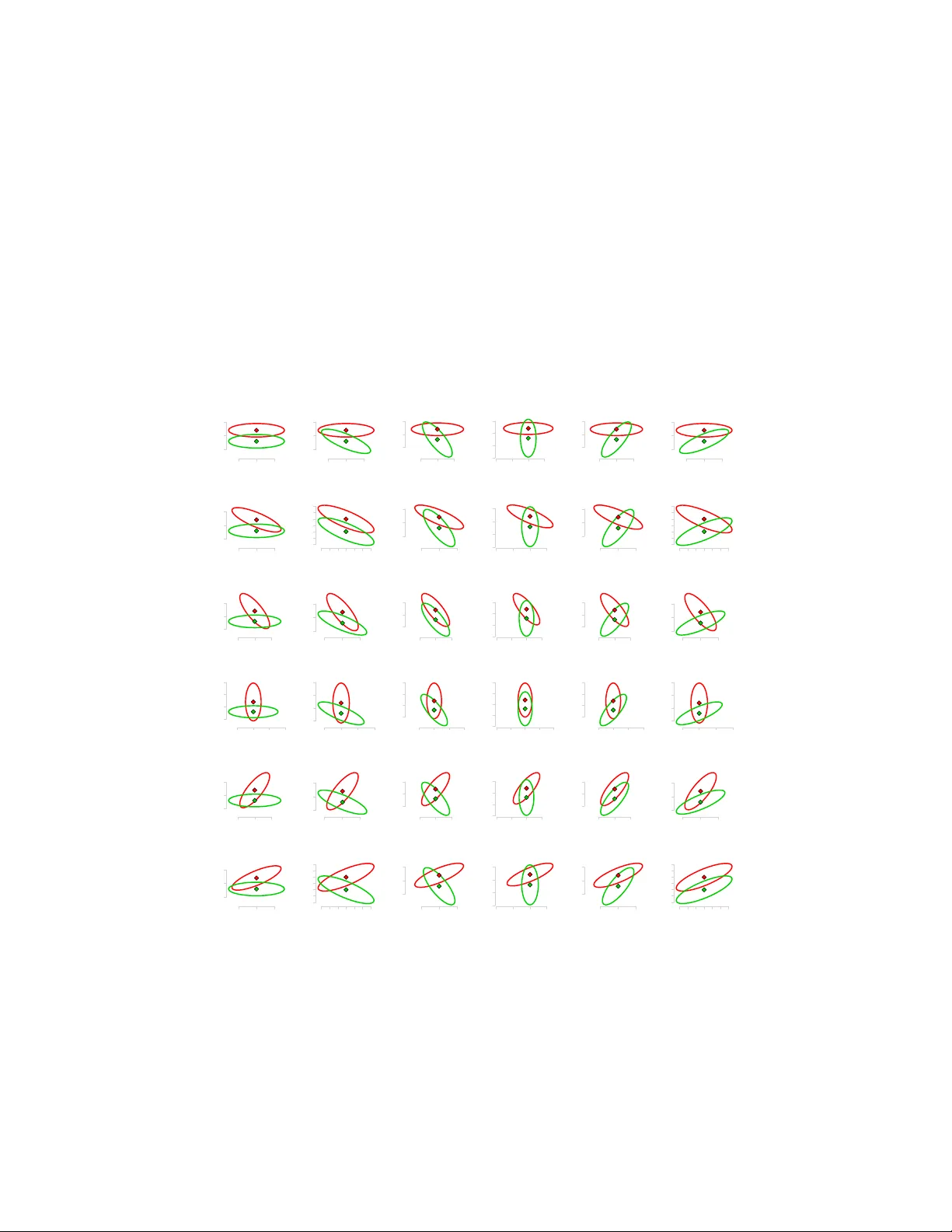
TRA CT ABLE MEASURE OF COMPONENT O VERLAP F OR GA USSIAN MIXTURE MODELS EW A NOW AKO WSKA, JA CEK KOR ONACKI, AND ST AN LIPOVETSKY Abstract. The ability to quantify distinctness of a cluster structure is fun- damental for certain simulation studies, in particular for those comparing per- formance of differen t classification algorithms. The intrinsic integral measure based on the ov erlap of corresp onding mixture components is often analyt- ically in tractable. This is also the case for Gaussian mixture mo dels with unequal co v ariance matrices when space dimension d > 1 . In this work we focus on Gaussian mixture mo dels and at the sample level we assume the class assignments to b e known. W e derive a measure of comp onent ov erlap based on eigenv alues of a generalized eigenproblem that represents Fisher’s discrim- inant task. W e explain rationale b ehind it and present simulation results that show how well it can reflect the b eha vior of the integral measure in its lin- ear approximation. The analyzed co efficien t p ossesses the adv antage of b eing analytically tractable and numerically computable even in complex setups. 1. Intr oduction 1.1. Ov erview. There are n umerous measures designed to capture distance be- t ween distributions or – more sp ecifically – ov erlap betw een comp onen ts of a Gauss- ian mixture mo del. One of the oldest is the Bhattac haryya co efficien t (see for instance [ 1 ] or [ 2 ]), which reflects the amount of o verlap betw een tw o statistical samples or distributions, a generalization of Mahalanobis distance describ ed in [ 3 ] or [ 4 ]. In the con text of information theory the most generic is the Kullback-Leibler div ergence (see [ 5 ]) – a non-symmetric measure of difference b etw een tw o distribu- tions, also interpreted as exp ected discrimination information, which sets the link with possible classification p erformance. In [ 6 ] an ov erlap coefficient is prop osed that measures agreement b et ween tw o distributions, it is applied to samples of data coming from normal distributions. Among more recent works, in [ 7 ] a c-separation measure b et w een m ultidimensional Gaussian distributions is defined, later dev el- op ed in [ 8 ] as exact-c-separation. In [ 9 ], in the setup simplified to tw o clusters k = 2 and t w o dimensions d = 2 , o verlap rate is defined as a ratio of the joint density in its saddle p oin t to its low er p eak. The concept of ridge curve is in tro duced and further developed in [ 10 ] and [ 11 ], generalized to arbitrary num b er of dimensions and clusters, turning the ridge curve in to a ridgeline manifold of the dimension k − 1 . All the measures use the parameters of the distributions to assess the o v erlap b et ween the comp onen ts and are typically formulated in terms of the underlying mo del. Ho wev er, they can also b e applied at the data level, as long as the class 2000 Mathematics Subje ct Classification. 62H30, 62E99. Key words and phrases. mixture mo del, cluster structure, ov erlap measure. Supported by National Science Center of Poland, DEC-2011/01/N/ST6/04174. 1 2 EW A NOW AKOWSKA, JACEK KORONACKI, AND ST AN LIPOVETSKY (or cluster) assignment is known. Then the mo del parameter estimates are used instead instead. 1.2. Con ten t. In Section 2 we recall the generic concept of comp onen t ov erlap and its b est linear appro ximation, we also show an example of an o v erlap assessment approac h and p oin t to common difficulties. Then, in Section 3 we in tro duce what w e refer to as Fisher’s distinctness measure and we explain rationale b ehind it. Finally , in Section 4 we show results of a sim ulation study that illustrates how w ell the Fisher’s co efficien t can reflect the linear appro ximation of the original in tractable ov erlap co efficien t. 2. O verlap of Distributions 2.1. In tegral measure. The most generic and natural co efficien t of ov erlap be- t ween components is what follows di rectly from the mixture definition: MLE err = 1 − Z R d max  π 1 f 1 ( µ 1 , Σ 1 ) , . . . , π k f k ( µ k , Σ k )  ( x )d x, whic h for k = 2 classes simplifies to (1) MLE err = Z R d min  π 1 f 1 ( µ 1 , Σ 1 ) , π 2 f 2 ( µ 2 , Σ 2 )  ( x )d x, where for d ≥ 1 by f i , i = 1 , . . . , k w e denote component densities and by π i , i = 1 , . . . , k their corresponding mixing factors. Throughout this work we will assume though that equal mixing factors are assigned to all the comp onents, which corresp onds to balanced cluster sizes at the sample level. Co efficien t ( 1 ) measures the actual ov erlap b etw een tw o probability distribution and for d = 1 is illustrated in Figure 1 . It coincides with in tuitive understanding of comp onen ts’ ov erlap and with its expected b eha vior — grows with increasing within cluster disp ersion (or v ariance, for d = 1 ) and decreasing distance betw ee n cluster cen ters. Also, it exhibits a strong link with classification p erformance, setting the upper limit for p ossible predictive accuracy in terms of maximum likelihoo d estimation (MLE) (see for instance [ 12 ]). Namely , b est classification pro cedures based on likelihoo d ratio (MLE) or — equiv alen tly — on its logarithm are given by (2) loglik ( f 1 , f 2 )( x ) = log  f 2 ( µ 2 , Σ 2 )( x ) f 1 ( µ 1 , Σ 1 )( x )  . Figure 1. Ov erlap (dark shadow) b et w een k = 2 Gaussian comp onen ts in d = 1 dimen- sion, concept illustration. F or the v alue of ( 2 ) less than a con- stan t observ ation x is classified to the first cluster, to the second otherwise. Hence the area of ov erlap b etw een the components, as given by 1 , cor- resp onds to the exp ected prop ortion of observ ations that are incorrectly classified by MLE-classification rule, based on the (estimated) parameters of the mixture. Therefore ( 1 ) is de- noted b y MLE err and alternativ ely referred to as MLE-misclassification or error rate. OVERLAP MEASURE FOR GAUSSIAN MIXTURE MODELS 3 The fundamen tal problem with formula ( 1 ), and also one of the reasons for n u- merous alternative approaches to o v erlap assessment, is that ( 1 ) is hardly tractable for mixtures with different cov ariance matrices in higher dimensions. Handling it analytically would require integrating functions of Gaussian density o ver regions whose description often do es not possess a tractable form ulaic description either. Therefore, it can only b e treated as a theoretical o v erlap co efficien t for Gaussian mixture mo dels and for practical applications replaced with other approaches. 2.2. Best linear appro ximation. The authors of [ 13 ] prop ose an approximation of ( 1 ) — b est linear separator for k = 2 Gaussian components in d ≥ 1 dimensions and an algorithm to determine it for a given data set X . They derive a linear function of x ∈ R d giv en by a vector b ∈ R d suc h that for a given constant c ∈ R inequalit y b T x ≤ c classifies observ ation x to the first cluster, while b T x > c to the second. V ector b and constant c are obtained iteratively in order to minimize maximal probabilit y of misclassification. As this approac h will be used in our sim ulations, it is describ ed b elo w in more details follo wing [ 13 ]. F or x coming from component l = 1 , 2 , b T x has a univ ariate normal distribution with mean b T µ l and v ariance b T Σ l b . As suc h, the probabilit y of misclassifying observ ation x when it comes from the first p opulation l = 1 equals (3) P 1  b T x > c  = P 1  b T x − b T µ 1 b T Σ 1 b > c − b T µ 1 b T Σ 1 b  = 1 − Φ  c − b T µ 1 b T Σ 1 b  = 1 − Φ  u 1  , where Φ denotes cum ulativ e distribution function for a univ ariate standardized normal distribution (cen tered at zero, with v ariance equal to one) and u 1 = c − b T µ 1 b T Σ 1 b . Similarly , probability of misclassifying observ ation x when it comes from the second p opulation l = 2 equals (4) P 2  b T x ≤ c  = P 1  b T x − b T µ 2 b T Σ 2 b ≤ c − b T µ 2 b T Σ 2 b  = = Φ  c − b T µ 2 b T Σ 2 b  = 1 − Φ  b T µ 2 − c b T Σ 2 b  = 1 − Φ ( u 2 ) , for u 2 = b T µ 2 − c b T Σ 2 b . As Φ is monotonic, the task max  P 1 ( u 1 ) , P 2 ( u 2 )  − → min b ∈ R d c ∈ R is equiv alen t to (5) min( u 1 , u 2 ) − → max b ∈ R d c ∈ R , whic h is more con v enient to work with. As the ob jectiv e is to find b ∈ R d and c ∈ R that minimize maximal probability of misclassification, we will refer to the resulting procedure as a minimax pro cedure. Analytical form ulation of admissible pro cedures for b and c leads to the following c haracterization (6) b = ( t 1 Σ 1 + t 2 Σ 2 ) − 1 ( µ 2 − µ 1 ) and (7) c = b T µ 1 + t 1 b T Σ 1 b = b T µ 2 − t 2 b T Σ 2 b, 4 EW A NOW AKOWSKA, JACEK KORONACKI, AND ST AN LIPOVETSKY where t 1 ∈ R and t 2 ∈ R are scalars. Minimax pro cedure is an admissible pro cedure with u 1 = u 2 . As such, for t = t 1 = (1 − t 2 ) the follo wing equality must hold (8) 0 = u 2 1 − u 2 2 = t 2 b T Σ 1 b − (1 − t ) 2 b T Σ 2 b = b T  t 2 Σ 1 − (1 − t ) 2 Σ 2  b. Equation ( 8 ) for t can b e solved n umerically by means of iterativ e pro cedure. With the ab o ve deriv ations, for a mixture of k = 2 comp onen ts in d ≥ 1 di- mensions with parameters µ 1 , Σ 1 and µ 2 , Σ 2 resp ectiv ely , the following algorithm pro vides best linear separator in terms of minimizing the maximal probability of misclassification. Algorithm 2.1: BestLinearSep ara tor ( µ 1 , Σ 1 , µ 2 , Σ 2 , pr ec ) initialize incr, crit, t rep eat calculate b with ( 6 ) calculate cr it with ( 8 ) if cr it > pr ec then t ← t − incr if cr it < − pr ec then t ← t + incr incr ← incr · 1 2 un til criterion cr it given by ( 8 ) met with exp ected precision pr ec calculate c with ( 7 ) calculate u 1 and u 2 and the probabilities of misclassification with ( 3 ) and ( 4 ) calculate ov erall probability of misclassification P minmax = max( P 1 ( u 1 ) , P 2 ( u 2 )) return ( P minmax , b, c, t ) Note that the v alue of assumed precision pr ec must b e given, while the v alues of scalar t , criterion cr it and increment incr must b e initialized. What is more, P minmax = P 1 ( u 1 ) = P 2 ( u 2 )) as for the minimax pro cedure u 1 = u 2 m ust hold. Note, that P minmax ma y b e considered a measure of o v erlap as a result of linear appro ximation of criterion ( 2 ). If Σ 1 = Σ 2 , formula ( 2 ) and its linear approximation giv en by b and c coincide, whic h is sure not the case for Σ 1 6 = Σ 2 . 2.3. The challenge of replacemen t. Degree of ov erlap b et ween mixture comp o- nen ts is critical for classification p erformance and must b e assessed for simulation purp oses and comparison of classification metho ds, hence the interest in the topic. There are man y measures prop osed in the literature that possess the prop ert y of b eing tractable ev en in a complex setup, how ever it is highly required that their b eha vior reflects the b eha vior of MLE err based either on ( 1 ) or on its linear approx- imation of the previous subsection. How ev er, this is not alwa ys the case, as shown in the b elo w example. E-distance. The metho d for o verlap assessmen t prop osed in [ 14 ] do es not as- sume underling normal mixture mo del, ho wev er it can b e very well applied in such setup. It is considered an extension to W ard’s minim um v ariance method (see [ 15 ]) that formally takes b oth into account — heterogeneit y betw een groups and homogeneit y within groups in data. F or this purp ose it uses joint b et w een-within e-distance b et ween clusters that constitutes the basis for agglomerative hierarchi- cal clustering pro cedure the authors prop ose. They define e- distanc e b et w een t w o OVERLAP MEASURE FOR GAUSSIAN MIXTURE MODELS 5 sets of observ ations X 1 = { x i 1 : c ( i 1 ) = 1 } , n 1 = | X 1 | and X 2 = { x i 2 : c ( i 2 ) = 2 } , n 2 = | X 2 | as (9) e( X 1 , X 2 ) = n 1 n 2 n 1 + n 2   2 n 1 n 2 X i 1 : c ( i 1 )=1 X i 2 : c ( i 2 )=2 k x i 1 − x i 2 k + − 1 n 2 1 X i 1 : c ( i 1 )=1 X j 1 : c ( j 1 )=1 k x i 1 − x j 1 k − 1 n 2 2 X i 2 : c ( i 2 )=2 X j 2 : c ( j 2 )=2 k x i 2 − x j 2 k   . The v alue of e-distance b et w een tw o resulting clusters may be considered a cluster structure distinctness measure. It is exp ected to reflect c hanges in within-cluster disp ersion and b et w een-cluster separation. It should also remain in tune with the theoretical structure distinctness measure giv en by likelihoo d ratio ( 2 ) or its linear appro ximation from [ 13 ]. 0.75 0.80 0.85 0.90 0.95 1.00 1.0 1.5 2.0 2.5 3.0 1.0 1.5 2.0 2.5 3.0 Clusterability ! heat map betw een ! cluster distance within ! cluster dispersion Figure 2. Heatmap — Anderson-Bahadur mis- classification error w/r to growing b et ween ( x - axis) and within ( y - axis) cluster disp ersion. 1000 1500 2000 2500 1.0 1.5 2.0 2.5 3.0 1.0 1.5 2.0 2.5 3.0 Sz ekel y ! Rizzo e ! distance ! heat map betw een ! cluster distance within ! cluster dispersion Figure 3. Heatmap — Szék ely-Rizzo e- distance ( 9 ) w/r to gro wing b et w een ( x -axis) and within ( y - axis) cluster disp ersion. Figures 2 and 3 compare v ariability of structure distinctness measures based on Anderson-Bahadur ([ 13 ]) and Székely-Rizzo ([ 14 ]) prop osals resp ectiv ely . The for- mer, similarly to the likelihoo d ratio theoretical distinctness measure, do es dep end on b oth — b etw een-cluster distance and within-cluster disp ersion, while the lat- ter essentially remains insensitive to within cluster dispersion, dep ending entirely on the b etw een class separation. This is an empirical insight which shows substan- tial discrepancy b et w een b ehavior of theoretical and intuitiv e structure distinctness measure and e-distance given b y ( 9 ), and hence p oin ts to another p oten tial difficulty when trying to replace the integral co efficien t. 6 EW A NOW AKOWSKA, JACEK KORONACKI, AND ST AN LIPOVETSKY 3. Fisher ’s distinctness measure 3.1. Mo del and notation. W e consider a data set X = ( x 1 , . . . , x n ) T , X ∈ R n × d of n observ ations coming from a mixture of k d -dimensional normal distributions f ( x ) = π 1 f 1 ( µ 1 , Σ 1 )( x ) + . . . + π k f k ( µ k , Σ k )( x ) , where f l ( µ l , Σ l )( x ) = 1 ( √ 2 π ) d √ det Σ l e − 1 2 ( x − µ l ) T Σ − 1 l ( x − µ l ) . W e call eac h f l ( µ l , Σ l ) , l = 1 , . . . , k a component of the mixture and each π l , l = 1 , . . . , k a mixing factor of the corresponding comp onent (see [ 12 ] or [ 16 ] and [ 17 ] or [ 18 ] for comparison with alternative approaches). W e assume that for all the comp onents equal mixing factors are assigned π 1 = · · · = π k = 1 k . Ho wev er, w e allow differen t co v ariance matrices Σ l . A dditionally , w e assume large space dimension with resp ect to the num b er of comp onen ts d > k − 1 and tak e the n umber of comp onen ts k and class assignments as known. W e use lo w er index to indicate data set when sample estimates of parameters are used. In particular, b y µ X ∈ R d w e denote sample mean and by Σ X ∈ R d × d co v ariance matrix for a data set X . F or notation ease we cen ter the data at the origin µ X = 0 . W e assume the cov ariance matrix to b e of full rank, rank( Σ X ) = d . Let T X = n Σ X b e the total scatter matrix for X . W e recall that a simple calculation (see for instance [ 12 ] or [ 19 ]) splits total scatter into its betw een and within cluster comp onen ts T X = B X + W X . By µ X,l and Σ X,l w e denote empirical mean and co v ariance matrix for class l , where l = 1 , . . . , k . By M X = ( µ X, 1 , . . . , µ X,k ) , M X ∈ R d × k w e understand a matrix of column v ectors of cluster means. W e assume the cluster means — as a set of p oin ts — to b e linearly indep enden t, so rank( M X ) = min( d, k − 1) = k − 1 . 3.2. Fisher’s task as an eigenproblem. Originally (see [ 20 ]), the separation was defined for 2 classes in single dimension v ∈ R d as the ratio of the v ariance b etw een the classes to the v ariance within the classes (10) F o ( v ) = v T B X v v T W X v . and then minimized ov er p ossible directions to find the linear subspace (Fisher’s discriminan t) that separates the classes b est v ∗ = argmin( F 0 ( v )) . F or our purp oses we will use the formulation (11) F ( v ) = 1 1 + 1 F o ( v ) = v T B X v v T T X v , whic h is equiv alent to ( 10 ) due to T X = B X + W X and yields the Fisher’s subspace b y maximizing o ver possible dimensions (12) v ∗ = argmax( F ( v )) . As m ultiplying v by a constant does not c hange the result of ( 12 ), it can alter- nativ ely b e expressed as a constrained optimization problem, namely (13) max v ∈ R d v T B X v sub ject to v T T X v = 1 . OVERLAP MEASURE FOR GAUSSIAN MIXTURE MODELS 7 The corresp onding Lagrange function defined as L ( v ; λ ) = v T B X v + λ  v T T X v − 1  yields ∂ L ( v ; λ ) ∂ v = 2 B X v − 2 λT X v = 0 , so (14) B X v = λT X v m ust hold at the solution. Problem ( 14 ) is a generalized eigenproblem for t wo matrices B X and T X . As we assume co v ariance matrix to b e w ell-defined, total scatter matrix T X is inv ertible, ho wev er T − 1 X B X is not necessarily symmetric so it is a priori not obvious if the eigenv alues are real. Hence, a decomp osition of the matrix T X is required to reduce the generalized eige nproblem to a standard eigenproblem for a transformed matrix. Solving a standard eigenproblem for T X w e obtain (15) T X = A T X L T X A T T X . Note, that A T X is orthonormal (i.e. A T X A T T X = I so A − 1 T X = A T T X ). Replacing in ( 14 ) matrix T X with its sp ectral decomposition ( 15 ) we get B X v = λA T X L T X A T T X v = λA T X L 1 / 2 T X L 1 / 2 T X A T T X v , then multiplying b y ( A T X L 1 / 2 T X ) − 1 from the left and by I in the middle we transform it to L − 1 / 2 T X A T T X B X A T X L − 1 / 2 T X L 1 / 2 T X A T T X v = λL 1 / 2 T X A T T X v . No w, substituting ˜ B = L − 1 / 2 T X A T T X B X A T X L − 1 / 2 T X =  L − 1 / 2 T X A T T X  B X  L − 1 / 2 T X A T T X  T and (16) ˜ v = L 1 / 2 T X A T T X v w e get a standard eigenproblem for ˜ B (17) ˜ B ˜ v = λ ˜ v . Solving ( 17 ) and using the inv erse transformation of ( 16 ) (18) v = A T X L − 1 / 2 T X ˜ v , w e obtain the solution v to the original problem ( 14 ), corresp onding to the same eigen v alue λ . In particular, it prov es that with our mo del assumptions ( 14 ) can b e reduced to a standard eigenproblem (19) T − 1 X B X v = λv , whic h takes the matrix form of (20)  T − 1 X B X  V = V L, where L ∈ R d × d is a diagonal matrix of eigenv alues in a non-decreasing order and V ∈ R d × d is a matrix of their corresp onding column eigenv ectors. Note that there is another alternative form ulation of the problem ( 14 ) via canon- ical correlation analysis (CCA), which may also come as a conv enient wa y to see 8 EW A NOW AKOWSKA, JACEK KORONACKI, AND ST AN LIPOVETSKY the task. In this setup Fisher’s eigen v alues corresp ond to squared canonical cor- relation co efficien ts. W e will not describ e it here in details but w e give references for interested readers. The approac h, referred to as canonical discriminan t analysis (CD A), w as first men tioned in [ 21 ] and thoroughly describ ed in [ 22 ]. The o v erview of classical CCA is giv en for instance in [ 12 ]. 3.3. Motiv ation. What we refer to as Fisher’s distinctness measure was inspired b y [ 23 ], where the idea of using the eigenproblem form ulation of the Fisher’s dis- crimination task and its resp ectiv e eigenv alues for assessing certain prop erties of data was used. As explained in Subsection 3.2 , Fisher’s discriminan t task can b e stated in terms of eigenproblem given by ( 20 ). Then, its ( k − 1) eigenv ectors corresp onding to the ( k − 1) non-zero eigen v alues span the Fisher’s subspace. Note that there are k − 1 non-zero eigen v alues as according to the mo del assumptions rank( T X ) = d and rank( B X ) = k − 1 and d > k − 1 . Due to ( 20 ) we ha v e V T T − 1 X B X V = L, so the eigenv alues capture v ariability in the spanning directions. As Fisher’s task is scale inv ariant, the increase in v ariabilit y may only b e due to increase in b et ween cluster scatter or decrease in within cluster scatter so it is expected to capture increase in structure distinctness very w ell. As squared canonical correlation co ef- ficien ts (see references in Subsection 3.2 ), the eigenv alues remain in the interv al of [0 , 1] whic h also makes them easy to compare and interpret. A dditionally , except for b eing easy to compute numerically , they are also conv enien t to handle analyt- ically , so they can easily b e used in sim ulations as well as formal deriv ations and justifications. What remains, is to prop ose function of the eigenv alues that could serv e as structure distinctness co efficien t and analyze its p erformance. This w as done by means of sim ulation study and describ ed in the next section. 4. Simula tion study 4.1. Ov erview. Due to its analytical complexity ( 1 ) is virtually intractable for mixtures with v aried co v ariance matrices (heterogeneous) or of higher space di- mension. How ev er, it relatively easy undergo es simulations of Mon te Carlo kind and can easily b e approximated n umerically with the b est linear approximation describ ed in subsection 2.2 . As suc h, it may b e used as a reference measure and replaced with another coefficient that reflects its b eha vior but offers the adv antage of b eing computable and analytically tractable, also in a more complex setup. The study was divided into tw o parts. In the first part tw o dimensional case was studied in details. Normal distribution was parametrized in a wa y that allow ed for easy parameter control. Then all the p ossible combinations w ere tested and the influence of change in betw een cluster separation and within cluster disp ersion was analysed. Three p ossible structure distinctness measures were compared — exact in tegral measure ( 1 ), its b est linear approximation describ ed in subsection 2.2 and Fisher’s eigenv alue. F or tw o dimensional data, the maxim um num b er of t w o clusters w as analysed (due to the assumption of d > k − 1 ), which led to one dimensional pro jections. Therefore, there w as just single Fisher’s eigen v alue to compare so the t w o dimensional step could not give grounds for function selection. The t w o dimensional study served as a thorough assessmen t of single Fisher’s eigen v alue p erformance. OVERLAP MEASURE FOR GAUSSIAN MIXTURE MODELS 9 In the second step multidimensional data was analyzed. Due to high n um b er of p ossible mixture parameter com binations only a random selection was considered. This step was meant to confirm satisfactory p erformance of Fisher eigen v alues as input for structure distinctness measure. Higher dimensionalit y allow ed for larger n umber of clusters, which resulted in ( k − 1) > 1 dimensionalit y of Fisher’s subspace. As such, it also gav e grounds for selecting appropriate function to transform ( k − 1) eigenv alues in to a single structure distinctness co efficient. Minim um λ X min and a verage ¯ λ X o ver Fisher’s non-zero eigenv alues were calculated as follows (21) λ X min = min j ∈{ 1 ,...,k − 1 } λ T − 1 X B X j and (22) ¯ λ X = 1 k − 1 k − 1 X j =1 λ T − 1 X B X j , and compared with the Monte Carlo estimates of the integral measure ( 1 ). Note that due to the larger num b er of classes allow ed, wider comparisons with the b est linear separator, defined for k = 2 only , w ere infeasible. Note that although the original concept ( 1 ) is defined in terms of ov erlap (simi- larit y) b et ween the comp onen ts, what is naturally captured by either minimum or a verage o ver non-zero Fisher’s eigen v alues, reflects the opp osite b eha vior, so should rather b e referred to as distinctness (dissimilarity) measure. Therefore we compare it with (1 − MLE err ) (or (1 − P minmax ) ), which is the probability of correct MLE classification (or its b est linear approximation). The transition from one to another is typically straightforw ard, how ever we p oin t that out explicitly to av oid confusion or additional transformations of the co efficien ts. Algorithm 4.1: TwoDimensionalD a t aGenera tion ( r, α, λ, q , k , N [] ) for each cluster l ∈ { 1 , . . . , k } do                                      commen t: Determine cluster center µ µ ←  r · sin  ( l − 1) · 2 π k  , r · cos  ( l − 1) · 2 π k  commen t: Compute cov ariance matrix Σ D ← diag ( λ, q · λ ) commen t: dispersion and shap e matrix R ←  cos( α ) − sin( α ) sin( α ) cos( α )  commen t: rotation matrix Σ ← RD R T commen t: Generate data dra w N [ l ] observ ations add cluster mean µ to each observ ation return ( data ) 4.2. T w o-dimensional sim ulations. T o allow for easy con trol ov er mixture pa- rameters, tw o dimensional mixture density was parametrized in a conv enien t wa y . Cluster centers were lo cated on a circle around origin (0 , 0) with radius r that 10 EW A NOW AKOWSKA, JACEK KORONACKI, AND ST AN LIPOVETSKY con trolled betw een cluster distance. T o allow for heterogeneit y , for eac h cluster co- v ariance matrix was determined separately . Within cluster disp ersion w as captured b y the leading eigenv alue λ = λ 1 , cluster shape by eigenv alues’ ratio q = λ 2 /λ 1 , and cluster rotation by rotation angle α . Based on these parameters for each com- p onen t mean vector and co v ariance matrix w ere computed. F or each comp onen t the data was generated with the algorithm based on Cholesky decomp osition, using affine transformation property for multiv ariate normal distribution. The detailed description of the algorithm is provided in [ 24 ]. Assuming the n um b er of clusters is giv en by k and N ∈ R k con tains desired cluster sizes, the ab o v e algorithm presen ts subsequen t steps of data generation. −5 0 5 −5 0 5 −5 0 5 −5 0 5 −5 0 5 −5 0 5 −5 0 5 10 −5 0 5 10 −5 0 5 −5 0 5 −5 0 5 −5 0 5 −5 0 5 −5 0 5 −6 −4 −2 0 2 4 6 −6 −2 2 4 6 −5 0 5 −5 0 5 −5 0 5 10 −5 0 5 10 −5 0 5 −5 0 5 −6 −4 −2 0 2 4 6 −6 −2 2 4 6 −5 0 5 −5 0 5 −5 0 5 −5 0 5 −5 0 5 −5 0 5 −5 0 5 10 −5 0 5 10 −5 0 5 −5 0 5 −5 0 5 −5 0 5 −10 −5 0 5 −10 −5 0 5 −10 −5 0 5 −10 −5 0 5 −10 −5 0 5 −10 −5 0 5 −10 −5 0 5 10 −10 −5 0 5 10 −10 −5 0 5 −10 −5 0 5 −10 −5 0 5 −10 −5 0 5 −5 0 5 −5 0 5 −5 0 5 −5 0 5 −5 0 5 −5 0 5 −5 0 5 10 −5 0 5 10 −5 0 5 −5 0 5 −5 0 5 −5 0 5 −5 0 5 −5 0 5 −6 −4 −2 0 2 4 6 −6 −2 2 4 6 −5 0 5 −5 0 5 −5 0 5 10 −5 0 5 10 −5 0 5 −5 0 5 −6 −4 −2 0 2 4 6 −6 −2 2 4 6 Figure 4. Design of tw o dimensional simulations — comp onen ts’ p osition with resp ect to each other. The simulation design is shown in Figure 4 , which presents all p ossible com bina- tions of comp onent p osition with resp ect to each other. Each of i = 1 , . . . , 6 ro ws corresp onds to i · π / 6 angle rotation for the first (red) component, while eac h of j = 1 , . . . , 6 columns corresp onds to j · π / 6 angle rotation for the second (green) OVERLAP MEASURE FOR GAUSSIAN MIXTURE MODELS 11 comp onen t. Altogether it yields 36 basic mixture p ositions. F or each p osition an influence of a single factor is analyzed and this includes in particular – increase in b et ween cluster distance (Figures 7 and 8 ), increase in within cluster disp ersion for b oth (Figures 9 and 10 ) and for first (Figures 11 and 12 ) and second (Figures 13 and 14 ) spanning direction only . The sp ecial case of spherical clusters is analyzed separately (Figures 15 to 18 ). All the results are av ailable in App endix, Section A . Figure 5. Impact of increasing b et w een cluster distance (second column) and within cluster dispersion (third column) for mixtures in p ositions as indicated in the first column. Red line indicates exact (integral) structure distinctness, green — its linear approxi- mate and blue — Fisher’s eigenv alue. Example of what can b e observed in all the charts is shown in Figure 5 . Even though the v alues for Fisher’s eigenv alue are muc h smaller, their v ariability reflects b eha vior of the integral measure to a large extent. It is even more in tune with the linear estimate, whic h is to b e exp ected given the linear nature of the Fisher’s discrimination task. Note, that the best linear approximate gives the upp er b ound on the precision with whic h a linear concept ma y reflect behavior of the non-linear in tegral measure. Also, it giv es upp er limit on classification accuracy using linear classifiers, which is the case of Fisher discriminant. Note also, that the comp onent p osition in the upp er row indicates homogeneit y (i.e. equal cov ariance matrices for b oth comp onen ts). This prop ert y is lost when within cluster v ariabilit y increases for one of the comp onen ts (last column). How ev er, it remains when only b etw een cluster distance is affected (middle column). Therefore, exact integral measure and its linear estimate ov erlap in this case. 12 EW A NOW AKOWSKA, JACEK KORONACKI, AND ST AN LIPOVETSKY 4.3. Multi-dimensional sim ulations. In higher dimensions direct analytical con- trol ov er distance and disp ersion of mixture parameters is muc h more complex. Ad- ditionally , there are many more com binations to examine. As such, the simulations w ere reduced to randomly chosen mixture parameters’ com binations corresp onding to the mixture p osition. F or each p osition the impact of increasing b et ween cluster distance and within cluster disp ersion was analysed. The study was designed to v erify adequacy of the information carried by the Fisher’s eigenv alues and to select its appropriate function to serve as the structure distinctness co efficient. Results are attac hed in App endix A in Figures 19 to 22 . In each row charts for random but fixed set of cluster means are presented. Similarly , the set of co v ariance ma- trices is random but fixed in each column. Mean vectors and cov ariance matrices in d dimensions were determined using R pack age clusterGeneration , which im- plemen ts the ideas describ ed in [ 25 ] and [ 26 ]. A dditionally , mean co ordinates are re-scaled to lie in the interv al [ − 3 √ d, 3 √ d ] which corresp onds to the range of the maxim um three standard deviations for co v ariance matrix. As such, the p ossible o verlap betw een comp onen ts stretches from complete to negligible. Figure 6. Effect of increasing b et w een cluster distance (left col- umn) and within cluster disp ersion (righ t column). Upper ro w giv es results for three dimensional simulations, while b ottom row for five dimensional case. Green line indicates Monte Carlo esti- mate of the integral structure distinctness, turquoise av erage non- zero Fisher’s eigen v alue, while blue — Fisher’s smallest non-zero eigen v alue. Again, what can b e observed in all the sim ulation plots in App endix A is illus- trated in Figure 6 . Behavior of av erage Fisher’s eigenv alue as given by ( 22 ) reflects v ariability of the integral measure. A t the same time, minimum non-zero Fisher’s eigen v alue ( 22 ) is less sensitive and therefore captures the changes in distinctness OVERLAP MEASURE FOR GAUSSIAN MIXTURE MODELS 13 to a lesser extent, which b ecomes even more apparent as the num b er of dimensions increases. As such, the a v erage non-zero Fisher’s eigen v alue tends to outperform the minimum non-zero Fisher’s eigen v alue and therefore the former shall b e recom- mended as the distinctness coeffici en t. 5. Conclusions. In this work we derive and motiv ate measure of distinctness (or alternatively – ov erlap) b et w een clusters of data, generated from a G aussian mixture model. The approach uses alternative form ulation of Fisher’s discrimination task, which is stated in terms of a generalized eigenproblem. W e sho w the task is w ell p osed in the context of the assumed mo del and can b e reduced to a standard eigenproblem with real eigen v alues. W e then express the distinctness coefficient as the a verage eigen v alue o v er the non-zero eigenv alues of the solution. W e compare the b eha v- ior of the co efficien t with the generic (in tegral) measure of structure distinctness defined in terms of the actual ov erlap b etw een the corresp onding distributions and its best linear appro ximation. Although the v alues of the Fisher’s co efficien t are lo wer than the v alues of actual ov erlap, their dynamic reflects very well the behav- ior of the generic integral measure and even b etter – its b est linear approximation. As opp osed to the generic integral measure and its b est linear approximation, the Fisher’s co efficien t offers the adv an tage of b eing not only numerically easily com- putable but also analytically tractable, even in a complex setup, regardless of the dimensionalit y of the space and heterogeneity of cov ariance matrices. References [1] A. Bhattacharyy a, On a measure of divergence betw een tw o statistical populations defined by their probability distributions, Bulletin of Cal. Math. So c. 35 (1) (1943) 99–109. [2] K. F ukunaga, Introduction to statistical pattern recognition, 2nd Edition, Computer Science and Scientific Computing, Academic Press, Inc., Boston, MA, 1990. [3] N. E. Da y , Estimating the components of a mixture of normal distributions , Biometrik a 56 (3) (1969) 463–474. URL http://www.jstor.org/stable/2 334652 [4] G. J. McLachlan, K. E. Basford, Mixture mo dels, V ol. 84 of Statistics: T extb ooks and Mono- graphs, Marcel Dekker, Inc., New Y ork, 1988, inference and applications to clustering. [5] S. Kullback, R. A. Leibler, On information and sufficiency , Ann. Math. Statistics 22 (1951) 79–86. doi:10.1214/aoms/1177729 694 . [6] H. F. Inman, E. L. Bradley , Jr., The ov erlapping co efficien t as a measure of agreement b etw een probability distributions and p oin t estimation of the ov erlap of tw o normal densities , Comm. Statist. Theory Metho ds 18 (10) (1989) 3851–3874. doi:10.1080/03610928908830127 . URL http://dx.doi.org/10.1080/036 10928908830127 [7] S. Dasgupta, Learning mixtures of gaussians, in: 40th Annual Symp osium on F oundations of Computer Science, 1999, pp. 634–644. doi:10.1109/SFFCS.1999.814639 . [8] R. Maitra, Initializing partition-optimization algorithms , IEEE/ACM T rans. Comput. Biol. Bioinformatics 6 (1) (2009) 144–157. doi:10.1109/TCBB.2007.70244 . URL http://dx.doi.org/10.1109/TCB B.2007.70244 [9] H.-J. Sun, M. Sun, S.-R. W ang, A measuremen t of ov erlap rate b et w een gaussiancomponents, in: In ternational Conference on Machine Learning and Cyb ernetics, V ol. 4, 2007, pp. 2373– 2378. doi:10.1109/ICMLC.2007.43 70542 . [10] S. Ray , B. G. Lindsay , The top ography of multiv ariate normal mixtures , Ann. Statist. 33 (5) (2005) 2042–2065. doi:10.1214/009053605000000417 . URL http://dx.doi.org/10.1214/009 053605000000417 [11] H. Sun, S. W a ng, Measuring the component ov erlapping in the Gaussian mixture mo del , Data Min. Knowl. Discov. 23 (3) (2011) 479–502. doi:10.1007/s10618- 011- 0212- 3 . URL http://dx.doi.org/10.1007/s10 618- 011- 0212- 3 14 EW A NOW AKOWSKA, JACEK KORONACKI, AND ST AN LIPOVETSKY [12] K. V. Mardia, J. T. Ken t, J. M. Bibby , Multiv ariate analysis, Academic Press [Harcourt Brace Jov a no vic h, Publishers], London-New Y ork-T oronto, Ont., 1979, probability and Mathemat- ical Statistics: A Series of Monographs and T extb ooks. [13] T. W. Anderson, R. R. Bahadur, Classification into t wo multiv ariate normal distributions with different cov ariance matrices , The Annals of Mathematical Statistics 33 (2) (1962) 420– 431. doi:10.1214/aoms/117770456 8 . URL http://dx.doi.org/10.1214/aom s/1177704568 [14] G. J. Székely , M. L. Rizzo, Hierarchical clustering via joint b et w een-within distances: ex- tending Ward’s minim um v ariance method , J. Classification 22 (2) (2005) 151–183. doi: 10.1007/s00357- 005- 0012- 9 . URL http://dx.doi.org/10.1007/s00 357- 005- 0012- 9 [15] J. H. W ard, Jr., Hierarchical grouping to optimize an ob jective function, J. Amer. Statist. Assoc. 58 (1963) 236–244. doi:10.2307/2282967 . [16] T. Hastie, R. Tibshirani, J. F riedman, The elemen ts of statistical learning , 2nd Edition, Springer Series in Statistics, Springer, New Y ork, 2009, data mining, inference, and prediction. doi:10.1007/978- 0- 387- 84858- 7 . URL http://dx.doi.org/10.1007/978- 0- 387- 84858- 7 [17] S. Lip o v etsky , A dditiv e and multiplicativ e mixed normal distributions and finding cluster centers , International Journal of Mac hine Learning and Cyb ernetics 4 (1) (2013) 1–11. doi: 10.1007/s13042- 012- 0070- 3 . URL http://dx.doi.org/10.1007/s130 42- 012- 0070- 3 [18] S. Lipovetsky , T otal o dds and other ob jectives for clustering via multinomial-logit model , Ad- v ances in Adaptiv e Data Analysis 04 (03) (2012) 1250019. doi:10.1142/S1793536912500197 . URL http://www.worldscientific.com /doi/abs/10.1142/S1793536912500197 [19] S. Lip ov etsky , Finding cluster centers and sizes via multinomial parameterization, Applied Mathematics and Computation 221 (2013) 571–580. doi:10.1016/j.amc.2013.06.098 . [20] R. Fisher, The use of multiple measurements in taxonomic problems , Annals of Eugenics 7 (2) (1936) 179–188. doi:10.1111/j.1469- 1809.1936.tb02137.x . URL http://dx.doi.org/10.111 1/j.1469- 1809.1936.tb02137.x [21] M. S. Bartlett, F urther asp ects of the theory of multiple regression , Mathematical Pro ceedings of the Cambridge Philosophical So ciety 34 (1938) 33–40. doi:10.1017/S030500410001 9897 . URL http://journals.cambridg e.org/article_S0305004100019897 [22] W. Dillon, M. Goldstein, Multiv ariate analysis: methods and applications, Wiley series in probability and mathematical statistics: Applied probability and statistics, Wiley , 1984. [23] S. Brubak er, S. V empala, Isotropic pca and affine-inv ariant clustering , in: M. Grötsc hel, G. Katona, G. Sági (Eds.), Building Bridges, V ol. 19 of Bolyai So ciet y Mathematical Studies, Springer Berlin Heidelb erg, 2008, pp. 241–281. doi:10.1007/978- 3- 540- 85221- 6_8 . URL http://dx.doi.org/10.1007/978- 3- 540- 85221- 6_8 [24] J. E. Gentle, Random num b er generation and Monte Carlo metho ds, 2nd Edition, Statistics and Computing, Springer, New Y ork, 2003. [25] H. Jo e, Generating random correlation matrices based on partial correlations , J. Multiv ariate Anal. 97 (10) (2006) 2177–2189. doi:10.1016/j.jmva.2005.05.010 . URL http://dx.doi.org/10.101 6/j.jmva.2005.05.010 [26] D. Kurowic k a, R. Cooke, Uncertaint y analysis with high dimensional dep endence mo delling , Wiley Series in Probability and Statistics, John Wiley & Sons, Ltd., Chichester, 2006. doi: 10.1002/0470863072 . URL http://dx.doi.org/10.100 2/0470863072 OVERLAP MEASURE FOR GAUSSIAN MIXTURE MODELS 15 Appendix A. Simula tion resul ts Ew a Now ako wska, Institute of Computer Science, Polish Academy of Sciences, ul. Jana Kazimierza 5, 01-248 W arsza w a, Poland E-mail address : ewa.nowakowska@ipipan.waw.pl Jacek K orona cki, Institute of Computer Science, Polish Academy of Sciences, ul. Jana Kazimierza 5, 01-248 W arsza w a, Poland E-mail address : jacek.koronacki@ipipan.waw.p l St an Lipovetsky, GfK Custom Research Nor th America, Marketing & Da t a Sci- ences, 8401 Golden V alley Rd., Minneapolis MN 55427, USA E-mail address : stan.lipovetsky@gfk.com 16 EW A NOW AKOWSKA, JACEK KORONACKI, AND ST AN LIPOVETSKY −5 0 5 −5 0 5 −5 0 5 −5 0 5 −5 0 5 −5 0 5 −5 0 5 −5 0 5 −5 0 5 −5 0 5 −5 0 5 −5 0 5 −5 0 5 −5 0 5 −5 0 5 −5 0 5 −5 0 5 −5 0 5 −5 0 5 −5 0 5 Figure 7. Diagram of increasing b et ween cluster distance 0 2 4 6 8 10 0.2 0.6 1.0 0 2 4 6 8 10 0.2 0.6 1.0 0 2 4 6 8 10 0.2 0.6 1.0 0 2 4 6 8 10 0.0 0.4 0.8 0 2 4 6 8 10 0.2 0.6 1.0 0 2 4 6 8 10 0.2 0.6 1.0 0 2 4 6 8 10 0.2 0.6 1.0 0 2 4 6 8 10 0.2 0.6 1.0 0 2 4 6 8 10 0.2 0.6 1.0 0 2 4 6 8 10 0.2 0.6 1.0 0 2 4 6 8 10 0.2 0.6 1.0 0 2 4 6 8 10 0.2 0.6 1.0 0 2 4 6 8 10 0.2 0.6 1.0 0 2 4 6 8 10 0.2 0.6 1.0 0 2 4 6 8 10 0.2 0.6 1.0 0 2 4 6 8 10 0.0 0.4 0.8 0 2 4 6 8 10 0.0 0.4 0.8 0 2 4 6 8 10 0.2 0.6 1.0 0 2 4 6 8 10 0.0 0.4 0.8 0 2 4 6 8 10 0.2 0.6 1.0 0 2 4 6 8 10 0.0 0.4 0.8 0 2 4 6 8 10 0.0 0.4 0.8 0 2 4 6 8 10 0.0 0.4 0.8 0 2 4 6 8 10 0.2 0.6 1.0 0 2 4 6 8 10 0.2 0.6 1.0 0 2 4 6 8 10 0.2 0.6 1.0 0 2 4 6 8 10 0.2 0.6 1.0 0 2 4 6 8 10 0.2 0.6 1.0 0 2 4 6 8 10 0.2 0.6 1.0 0 2 4 6 8 10 0.2 0.6 1.0 0 2 4 6 8 10 0.2 0.6 1.0 0 2 4 6 8 10 0.2 0.6 1.0 0 2 4 6 8 10 0.0 0.4 0.8 0 2 4 6 8 10 0.0 0.4 0.8 0 2 4 6 8 10 0.2 0.6 1.0 0 2 4 6 8 10 0.2 0.6 1.0 Figure 8. F or clusters in p osition as in Figure 4 , eac h c hart presen ts impact of increasing b et w een cluster distance according to the pattern from Figure 7 , measured with exact (1 − MLE err ) (red), its linear approximation (1 − P minmax ) (green) and Fisher’s eigen v alue (blue). OVERLAP MEASURE FOR GAUSSIAN MIXTURE MODELS 17 −5 0 5 −5 0 5 −5 0 5 −5 0 5 −5 0 5 −5 0 5 −5 0 5 −5 0 5 −10 −5 0 5 10 −10 −5 0 5 10 −10 −5 0 5 10 −10 −5 0 5 10 −10 −5 0 5 10 −10 −5 0 5 10 −10 −5 0 5 10 −10 0 5 10 −10 −5 0 5 10 −10 0 5 10 −10 −5 0 5 10 −10 0 5 10 Figure 9. Diagram of increasing within cluster disp ersion – in b oth spanning directions 0 2 4 6 8 10 0.70 0.85 1.00 0 2 4 6 8 10 0.6 0.8 1.0 0 2 4 6 8 10 0.3 0.6 0.9 0 2 4 6 8 10 0.2 0.6 0 2 4 6 8 10 0.3 0.6 0.9 0 2 4 6 8 10 0.6 0.8 1.0 0 2 4 6 8 10 0.6 0.8 0 2 4 6 8 10 0.6 0.8 1.0 0 2 4 6 8 10 0.4 0.6 0.8 0 2 4 6 8 10 0.2 0.6 0 2 4 6 8 10 0.3 0.6 0.9 0 2 4 6 8 10 0.5 0.7 0.9 0 2 4 6 8 10 0.5 0.7 0.9 0 2 4 6 8 10 0.5 0.7 0.9 0 2 4 6 8 10 0.4 0.6 0.8 0 2 4 6 8 10 0.2 0.5 0.8 0 2 4 6 8 10 0.2 0.5 0.8 0 2 4 6 8 10 0.4 0.6 0.8 0 2 4 6 8 10 0.4 0.6 0.8 0 2 4 6 8 10 0.4 0.6 0.8 0 2 4 6 8 10 0.3 0.6 0.9 0 2 4 6 8 10 0.2 0.5 0.8 0 2 4 6 8 10 0.3 0.5 0.7 0 2 4 6 8 10 0.4 0.6 0.8 0 2 4 6 8 10 0.5 0.7 0.9 0 2 4 6 8 10 0.4 0.6 0.8 0 2 4 6 8 10 0.2 0.5 0.8 0 2 4 6 8 10 0.2 0.5 0.8 0 2 4 6 8 10 0.4 0.6 0.8 0 2 4 6 8 10 0.5 0.7 0.9 0 2 4 6 8 10 0.6 0.8 0 2 4 6 8 10 0.5 0.7 0.9 0 2 4 6 8 10 0.3 0.6 0.9 0 2 4 6 8 10 0.2 0.6 0 2 4 6 8 10 0.4 0.6 0.8 0 2 4 6 8 10 0.6 0.8 1.0 Figure 10. F or clusters in position as in Figure 4 , each c hart presen ts impact of increasing within cluster disp ersion (b oth di- rections) according to the pattern from Figure 9 , measured with exact (1 − MLE err ) (red), its linear appro ximation (1 − P minmax ) (green) and Fisher’s eigenv alue (blue). 18 EW A NOW AKOWSKA, JACEK KORONACKI, AND ST AN LIPOVETSKY −5 0 5 −5 0 5 −5 0 5 −5 0 5 −5 0 5 −5 0 5 −5 0 5 −5 0 5 −10 −5 0 5 10 −10 −5 0 5 10 −10 −5 0 5 10 −10 −5 0 5 10 −10 −5 0 5 10 −10 −5 0 5 10 −10 −5 0 5 10 −10 0 5 10 −10 −5 0 5 10 −10 0 5 10 −10 −5 0 5 10 −10 0 5 10 Figure 11. Diagram of increasing within cluster disp ersion – first spanning direction 0 2 4 6 8 10 0.80 0.90 0 2 4 6 8 10 0.65 0.85 0 2 4 6 8 10 0.4 0.7 0 2 4 6 8 10 0.2 0.6 0 2 4 6 8 10 0.4 0.7 0 2 4 6 8 10 0.65 0.80 0.95 0 2 4 6 8 10 0.65 0.80 0.95 0 2 4 6 8 10 0.75 0.85 0.95 0 2 4 6 8 10 0.5 0.7 0.9 0 2 4 6 8 10 0.2 0.6 0 2 4 6 8 10 0.3 0.6 0.9 0 2 4 6 8 10 0.5 0.7 0.9 0 2 4 6 8 10 0.5 0.7 0.9 0 2 4 6 8 10 0.60 0.75 0.90 0 2 4 6 8 10 0.6 0.8 0 2 4 6 8 10 0.2 0.5 0.8 0 2 4 6 8 10 0.3 0.6 0.9 0 2 4 6 8 10 0.4 0.6 0.8 0 2 4 6 8 10 0.4 0.6 0.8 0 2 4 6 8 10 0.4 0.6 0.8 0 2 4 6 8 10 0.3 0.5 0.7 0 2 4 6 8 10 0.2 0.5 0.8 0 2 4 6 8 10 0.4 0.6 0.8 0 2 4 6 8 10 0.4 0.6 0.8 0 2 4 6 8 10 0.5 0.7 0.9 0 2 4 6 8 10 0.4 0.6 0.8 0 2 4 6 8 10 0.3 0.6 0 2 4 6 8 10 0.2 0.5 0.8 0 2 4 6 8 10 0.6 0.8 0 2 4 6 8 10 0.60 0.75 0.90 0 2 4 6 8 10 0.70 0.85 0 2 4 6 8 10 0.5 0.7 0.9 0 2 4 6 8 10 0.3 0.6 0.9 0 2 4 6 8 10 0.2 0.6 0 2 4 6 8 10 0.5 0.7 0.9 0 2 4 6 8 10 0.75 0.85 0.95 Figure 12. F or clusters in position as in Figure 4 , each c hart presen ts impact of increasing within cluster disp ersion (first direc- tion) according to the pattern from Figure 11 , measured with exact (1 − MLE err ) (red), its linear approximation (1 − P minmax ) (green) and Fisher’s eigen v alue (blue). OVERLAP MEASURE FOR GAUSSIAN MIXTURE MODELS 19 −5 0 5 −5 0 5 −5 0 5 −5 0 5 −5 0 5 −5 0 5 −5 0 5 10 −5 0 5 10 −10 0 5 10 −10 0 5 10 15 −20 0 10 20 −20 −10 0 10 20 −20 0 10 20 −20 0 10 20 Figure 13. Diagram of increasing within cluster disp ersion – second spanning direction 0 2 4 6 8 0.2 0.6 1.0 0 2 4 6 8 0.2 0.6 0 2 4 6 8 0.4 0.6 0.8 0 2 4 6 8 0.4 0.6 0.8 0 2 4 6 8 0.3 0.6 0.9 0 2 4 6 8 0.2 0.6 0 2 4 6 8 0.2 0.6 0 2 4 6 8 0.2 0.6 0 2 4 6 8 0.3 0.6 0.9 0 2 4 6 8 0.4 0.6 0.8 0 2 4 6 8 0.4 0.6 0.8 0 2 4 6 8 0.2 0.6 0 2 4 6 8 0.2 0.6 0 2 4 6 8 0.2 0.6 0 2 4 6 8 0.3 0.6 0.9 0 2 4 6 8 0.3 0.6 0.9 0 2 4 6 8 0.3 0.6 0.9 0 2 4 6 8 0.2 0.5 0.8 0 2 4 6 8 0.2 0.6 0 2 4 6 8 0.2 0.6 0 2 4 6 8 0.3 0.6 0.9 0 2 4 6 8 0.3 0.6 0.9 0 2 4 6 8 0.3 0.6 0.9 0 2 4 6 8 0.2 0.6 0 2 4 6 8 0.2 0.6 0 2 4 6 8 0.2 0.5 0.8 0 2 4 6 8 0.3 0.6 0.9 0 2 4 6 8 0.3 0.6 0.9 0 2 4 6 8 0.3 0.6 0.9 0 2 4 6 8 0.2 0.6 0 2 4 6 8 0.2 0.6 0 2 4 6 8 0.2 0.5 0.8 0 2 4 6 8 0.4 0.6 0.8 0 2 4 6 8 0.4 0.6 0.8 0 2 4 6 8 0.3 0.6 0.9 0 2 4 6 8 0.2 0.6 Figure 14. F or clusters in position as in Figure 4 , each c hart presen ts impact of increasing within cluster disp ersion (second di- rection) according to the pattern from Figure 13 , measured with exact (1 − MLE err ) (red), its linear appro ximation (1 − P minmax ) (green) and Fisher’s eigenv alue (blue). 20 EW A NOW AKOWSKA, JACEK KORONACKI, AND ST AN LIPOVETSKY −3 −2 −1 0 1 2 3 −3 −2 −1 0 1 2 3 −4 −2 0 2 4 −4 −2 0 2 4 −4 −2 0 2 4 −4 −2 0 2 4 −6 −4 −2 0 2 4 6 −6 −4 −2 0 2 4 6 −5 0 5 −5 0 5 Figure 15. Spherical comp onen ts – diagram of increasing b e- t ween cluster distance −4 −2 0 2 4 −4 −2 0 2 4 −5 0 5 −5 0 5 −10 −5 0 5 10 −10 −5 0 5 10 −10 −5 0 5 10 −10 −5 0 5 10 −15 −10 −5 0 5 10 15 −15 −10 −5 0 5 10 15 Figure 16. Diagram of balanced increase in within cluster dis- p ersion (same increase for b oth clusters) −5 0 5 −5 0 5 −5 0 5 10 −5 0 5 10 −5 0 5 10 −5 0 5 10 −10 −5 0 5 10 15 −10 −5 0 5 10 15 −10 −5 0 5 10 15 −10 −5 0 5 10 15 Figure 17. Diagram of unbalanced increase in within cluster disp ersion (increase for one cluster only) 0 1 2 3 4 5 6 0.0 0.2 0.4 0.6 0.8 1.0 0 1 2 3 4 5 6 0.0 0.2 0.4 0.6 0.8 1.0 0 1 2 3 4 5 6 0.0 0.2 0.4 0.6 0.8 1.0 0 1 2 3 4 5 6 0.0 0.2 0.4 0.6 0.8 1.0 0 1 2 3 4 5 6 0.0 0.2 0.4 0.6 0.8 1.0 0 1 2 3 4 5 6 0.0 0.2 0.4 0.6 0.8 1.0 0 1 2 3 4 5 6 0.0 0.2 0.4 0.6 0.8 1.0 0 1 2 3 4 5 6 0.0 0.2 0.4 0.6 0.8 1.0 0 1 2 3 4 5 6 0.0 0.2 0.4 0.6 0.8 1.0 0 1 2 3 4 5 6 0.0 0.2 0.4 0.6 0.8 1.0 Figure 18. F or s pherical clusters, each line follows the distance pattern from Figure 15 , eac h chart presents impact of increasing within cluster disp ersion – balanced in the first line (Figure 16 , un balanced in the second (Figure 17 ), measured with exact (1 − MLE err ) (red), its linear approximation (1 − P minmax ) (green) and Fisher’s eigenv alue (blue). OVERLAP MEASURE FOR GAUSSIAN MIXTURE MODELS 21 0 2 4 6 8 10 0.0 0.2 0.4 0.6 0.8 1.0 0 2 4 6 8 10 0.0 0.2 0.4 0.6 0.8 1.0 0 2 4 6 8 10 0.0 0.2 0.4 0.6 0.8 1.0 0 2 4 6 8 10 0.0 0.2 0.4 0.6 0.8 1.0 0 2 4 6 8 10 0.0 0.2 0.4 0.6 0.8 1.0 0 2 4 6 8 10 0.0 0.2 0.4 0.6 0.8 1.0 0 2 4 6 8 10 0.0 0.2 0.4 0.6 0.8 1.0 0 2 4 6 8 10 0.0 0.2 0.4 0.6 0.8 1.0 0 2 4 6 8 10 0.0 0.2 0.4 0.6 0.8 1.0 0 2 4 6 8 10 0.0 0.2 0.4 0.6 0.8 1.0 0 2 4 6 8 10 0.0 0.2 0.4 0.6 0.8 1.0 0 2 4 6 8 10 0.0 0.2 0.4 0.6 0.8 1.0 0 2 4 6 8 10 0.0 0.2 0.4 0.6 0.8 1.0 0 2 4 6 8 10 0.0 0.2 0.4 0.6 0.8 1.0 0 2 4 6 8 10 0.0 0.2 0.4 0.6 0.8 1.0 0 2 4 6 8 10 0.0 0.2 0.4 0.6 0.8 1.0 0 2 4 6 8 10 0.0 0.2 0.4 0.6 0.8 1.0 0 2 4 6 8 10 0.0 0.2 0.4 0.6 0.8 1.0 0 2 4 6 8 10 0.0 0.2 0.4 0.6 0.8 1.0 0 2 4 6 8 10 0.0 0.2 0.4 0.6 0.8 1.0 0 2 4 6 8 10 0.0 0.2 0.4 0.6 0.8 1.0 0 2 4 6 8 10 0.0 0.2 0.4 0.6 0.8 1.0 0 2 4 6 8 10 0.0 0.2 0.4 0.6 0.8 1.0 0 2 4 6 8 10 0.0 0.2 0.4 0.6 0.8 1.0 0 2 4 6 8 10 0.0 0.2 0.4 0.6 0.8 1.0 Figure 19. Three dimensions: for random (but fixed in eac h ro w) set of cluster means and random (but fixed in each column) set of cov ariance matrices, eac h c hart presents impact of increas- ing b et w een cluster distance , measured with exact integral mea- sure (green), a v erage Fisher’s eigenv alue (turquoise) and minim um Fisher’s eigenv alue (blue). 22 EW A NOW AKOWSKA, JACEK KORONACKI, AND ST AN LIPOVETSKY 0 2 4 6 8 10 0.0 0.2 0.4 0.6 0.8 1.0 0 2 4 6 8 10 0.0 0.2 0.4 0.6 0.8 1.0 0 2 4 6 8 10 0.0 0.2 0.4 0.6 0.8 1.0 0 2 4 6 8 10 0.0 0.2 0.4 0.6 0.8 1.0 0 2 4 6 8 10 0.0 0.2 0.4 0.6 0.8 1.0 0 2 4 6 8 10 0.0 0.2 0.4 0.6 0.8 1.0 0 2 4 6 8 10 0.0 0.2 0.4 0.6 0.8 1.0 0 2 4 6 8 10 0.0 0.2 0.4 0.6 0.8 1.0 0 2 4 6 8 10 0.0 0.2 0.4 0.6 0.8 1.0 0 2 4 6 8 10 0.0 0.2 0.4 0.6 0.8 1.0 0 2 4 6 8 10 0.0 0.2 0.4 0.6 0.8 1.0 0 2 4 6 8 10 0.0 0.2 0.4 0.6 0.8 1.0 0 2 4 6 8 10 0.0 0.2 0.4 0.6 0.8 1.0 0 2 4 6 8 10 0.0 0.2 0.4 0.6 0.8 1.0 0 2 4 6 8 10 0.0 0.2 0.4 0.6 0.8 1.0 0 2 4 6 8 10 0.0 0.2 0.4 0.6 0.8 1.0 0 2 4 6 8 10 0.0 0.2 0.4 0.6 0.8 1.0 0 2 4 6 8 10 0.0 0.2 0.4 0.6 0.8 1.0 0 2 4 6 8 10 0.0 0.2 0.4 0.6 0.8 1.0 0 2 4 6 8 10 0.0 0.2 0.4 0.6 0.8 1.0 0 2 4 6 8 10 0.0 0.2 0.4 0.6 0.8 1.0 0 2 4 6 8 10 0.0 0.2 0.4 0.6 0.8 1.0 0 2 4 6 8 10 0.0 0.2 0.4 0.6 0.8 1.0 0 2 4 6 8 10 0.0 0.2 0.4 0.6 0.8 1.0 0 2 4 6 8 10 0.0 0.2 0.4 0.6 0.8 1.0 Figure 20. Five dimensions: for random (but fixed in each row) set of cluster means and random (but fixed in eac h column) set of cov ariance matrices, each c hart presents impact of increas- ing b et w een cluster distance , measured with exact integral mea- sure (green), a v erage Fisher’s eigenv alue (turquoise) and minim um Fisher’s eigenv alue (blue). OVERLAP MEASURE FOR GAUSSIAN MIXTURE MODELS 23 0 2 4 6 8 10 0.0 0.2 0.4 0.6 0.8 1.0 0 2 4 6 8 10 0.0 0.2 0.4 0.6 0.8 1.0 0 2 4 6 8 10 0.0 0.2 0.4 0.6 0.8 1.0 0 2 4 6 8 10 0.0 0.2 0.4 0.6 0.8 1.0 0 2 4 6 8 10 0.0 0.2 0.4 0.6 0.8 1.0 0 2 4 6 8 10 0.0 0.2 0.4 0.6 0.8 1.0 0 2 4 6 8 10 0.0 0.2 0.4 0.6 0.8 1.0 0 2 4 6 8 10 0.0 0.2 0.4 0.6 0.8 1.0 0 2 4 6 8 10 0.0 0.2 0.4 0.6 0.8 1.0 0 2 4 6 8 10 0.0 0.2 0.4 0.6 0.8 1.0 0 2 4 6 8 10 0.0 0.2 0.4 0.6 0.8 1.0 0 2 4 6 8 10 0.0 0.2 0.4 0.6 0.8 1.0 0 2 4 6 8 10 0.0 0.2 0.4 0.6 0.8 1.0 0 2 4 6 8 10 0.0 0.2 0.4 0.6 0.8 1.0 0 2 4 6 8 10 0.0 0.2 0.4 0.6 0.8 1.0 0 2 4 6 8 10 0.0 0.2 0.4 0.6 0.8 1.0 0 2 4 6 8 10 0.0 0.2 0.4 0.6 0.8 1.0 0 2 4 6 8 10 0.0 0.2 0.4 0.6 0.8 1.0 0 2 4 6 8 10 0.0 0.2 0.4 0.6 0.8 1.0 0 2 4 6 8 10 0.0 0.2 0.4 0.6 0.8 1.0 0 2 4 6 8 10 0.0 0.2 0.4 0.6 0.8 1.0 0 2 4 6 8 10 0.0 0.2 0.4 0.6 0.8 1.0 0 2 4 6 8 10 0.0 0.2 0.4 0.6 0.8 1.0 0 2 4 6 8 10 0.0 0.2 0.4 0.6 0.8 1.0 0 2 4 6 8 10 0.0 0.2 0.4 0.6 0.8 1.0 Figure 21. Three dimensions: for random (but fixed in eac h ro w) set of cluster means and random (but fixed in each column) set of cov ariance matrices, eac h c hart presents impact of increas- ing within cluster disp ersion , measured w ith exact integral mea- sure (green), a v erage Fisher’s eigenv alue (turquoise) and minim um Fisher’s eigenv alue (blue). 24 EW A NOW AKOWSKA, JACEK KORONACKI, AND ST AN LIPOVETSKY 0 2 4 6 8 10 0.0 0.2 0.4 0.6 0.8 1.0 0 2 4 6 8 10 0.0 0.2 0.4 0.6 0.8 1.0 0 2 4 6 8 10 0.0 0.2 0.4 0.6 0.8 1.0 0 2 4 6 8 10 0.0 0.2 0.4 0.6 0.8 1.0 0 2 4 6 8 10 0.0 0.2 0.4 0.6 0.8 1.0 0 2 4 6 8 10 0.0 0.2 0.4 0.6 0.8 1.0 0 2 4 6 8 10 0.0 0.2 0.4 0.6 0.8 1.0 0 2 4 6 8 10 0.0 0.2 0.4 0.6 0.8 1.0 0 2 4 6 8 10 0.0 0.2 0.4 0.6 0.8 1.0 0 2 4 6 8 10 0.0 0.2 0.4 0.6 0.8 1.0 0 2 4 6 8 10 0.0 0.2 0.4 0.6 0.8 1.0 0 2 4 6 8 10 0.0 0.2 0.4 0.6 0.8 1.0 0 2 4 6 8 10 0.0 0.2 0.4 0.6 0.8 1.0 0 2 4 6 8 10 0.0 0.2 0.4 0.6 0.8 1.0 0 2 4 6 8 10 0.0 0.2 0.4 0.6 0.8 1.0 0 2 4 6 8 10 0.0 0.2 0.4 0.6 0.8 1.0 0 2 4 6 8 10 0.0 0.2 0.4 0.6 0.8 1.0 0 2 4 6 8 10 0.0 0.2 0.4 0.6 0.8 1.0 0 2 4 6 8 10 0.0 0.2 0.4 0.6 0.8 1.0 0 2 4 6 8 10 0.0 0.2 0.4 0.6 0.8 1.0 0 2 4 6 8 10 0.0 0.2 0.4 0.6 0.8 1.0 0 2 4 6 8 10 0.0 0.2 0.4 0.6 0.8 1.0 0 2 4 6 8 10 0.0 0.2 0.4 0.6 0.8 1.0 0 2 4 6 8 10 0.0 0.2 0.4 0.6 0.8 1.0 0 2 4 6 8 10 0.0 0.2 0.4 0.6 0.8 1.0 Figure 22. Five dimensions: for random (but fixed in each row) set of cluster means and random (but fixed in eac h column) set of cov ariance matrices, eac h chart presents impact of increasing within cluster disp ersion , measured with exact integral mea- sure (green), a v erage Fisher’s eigenv alue (turquoise) and minim um Fisher’s eigenv alue (blue).