Mutual Information and Conditional Mean Prediction Error

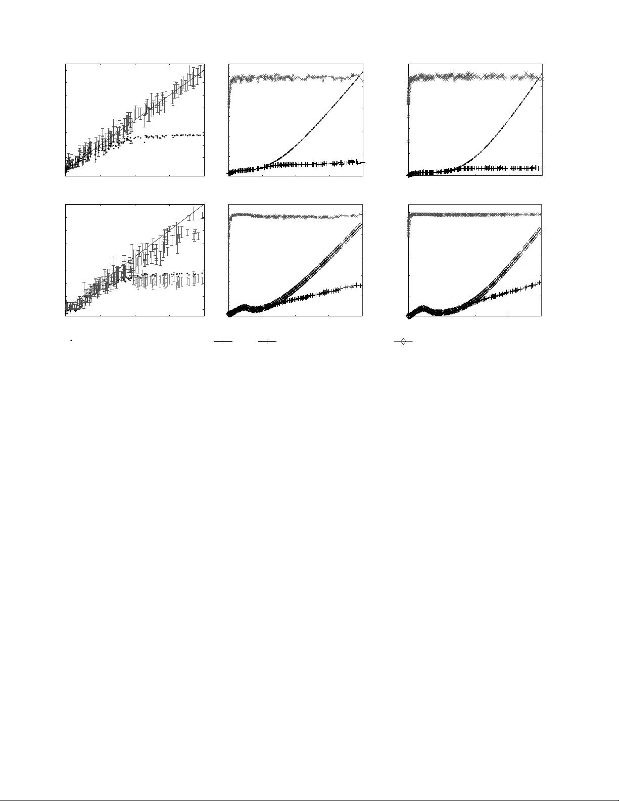
1 Mutual Inf ormation and Conditional Mean Prediction Err or Cli ve G. Bowsher 1 and Margaritis V oliotis School of Mathematics, Uni versity of Bristol, U.K. Abstract Mutual information is fundamentally important for measuring statistical dependence between variables and for quantifying information transfer by signaling and communication mechanisms. It can, howe ver , be challenging to ev aluate for physical models of such mechanisms and to estimate reliably from data. Furthermore, its relationship to better known statistical procedures is still poorly understood. Here we explore ne w connections between mutual information and regression-based dependence measures, ν − 1 , that utilise the determinant of the second-moment matrix of the conditional mean prediction error . W e examine conv ergence properties as ν → 0 and establish sharp lower bounds on mutual information and capacity of the form log( ν − 1 / 2 ) . The bounds are tighter than lo wer bounds based on the Pearson correlation and ones deriv ed using average mean square-error rate distortion ar guments. Furthermore, their estimation is feasible using techniques from nonparametric regression. As an illustration we provide bootstrap confidence interv als for the lo wer bounds which, through use of a composite estimator , substantially improv e upon inference about mutual information based on k -nearest neighbour estimators alone. Index T erms Lower bound on mutual information, relati ve entropy , information capacity , nearest-neighbour estimator , corre- lation and dependence measures, regression. I . I N T R O D U C T I O N Mutual information is fundamentally important for measuring statistical dependence between variables [ 1 ], [ 2 ], [ 3 ], [ 4 ], and for quantifying information transfer by engineered or naturally occurring communication systems [ 5 ], [ 6 ]. Statistical analysis using mutual information has been particularly influential in neuroscience [ 7 ], and is becom- ing so in systems biology for studying the biomolecular signaling networks used by cells to detect, process and act upon the chemical signals they receiv e [ 8 ], [ 9 ], [ 10 ]. It can, howe ver , be challenging to estimate mutual information reliably with a v ailable sample sizes [ 11 ], and difficult to derive mutual information and capacity e xactly using mechanistic models of the ‘channels’ via which signals are conv eyed. Furthermore, connections between mutual information and better known statistical procedures such as regression, and their associated dependence measures, are still poorly understood. In order to address these challenges, the relationship between mutual information and the error incurred by estimation (or ‘prediction’) using the conditional mean is now receiving attention. The focus has been on minimum mean square estimation error or , more generally , its average across the elements of the vector being estimated [ 12 ], [ 13 ], [ 14 ]. Instead, we focus on connections between mutual information and regression- based dependence measures, ν − 1 , that utilise the determinant of the second-moment matrix of the conditional mean prediction error . W e examine con vergence properties as ν → 0 , and establish sharp lower bounds on mutual information of the form log( ν − 1 / 2 ) . The bounds are tighter than lower bounds based on the Pearson correlation and ones deri ved using average mean square-error rate distortion arguments. The mutual information between 2 random vectors X and Z , written I ( X ; Z ) , is the Kullback-Leibler div ergence between their joint distribution and the product of their marginal distributions [ 15 ]. Mutual information thus measures the div ergence between the joint distribution of ( X, Z ) and the distrib ution in which X and Z are independent but hav e the same marginals. I ( X ; Z ) has desirable properties as a measure of statistical dependence: it satisfies (after monotonic transformation) all 7 of R ´ enyi’ s postulates [ 16 ] for a dependence measure between 2 random v ariables, and underlies the recently introduced maximal information coefficient [ 4 ] for detecting pairwise associations in large data sets. Importantly , mutual information captures nonlinear dependence and dependence arising from moments higher than the conditional mean. A decision-theoretic interpretation is indicative of the broad applicability of mutual information as a summary measure of statistical dependence. It can be shown [ 17 ] that I ( X ; Z ) is equal to the increase in expected utility from 1 corresponding author: c.bo wsher@bristol.ac.uk 2 reporting the posterior distribution of either of the two random vectors based on observation of the other , compared to reporting its marginal distribution—for example, reporting p ( Z | X = x ) instead of p ( Z ) . This holds when the utility function is a smooth, proper , local score function—as appropriate for scientific reporting of distributions as ‘pure inferences’ [ 18 ]—because the logarithmic score function is the only score function having all these properties. In information theory , the supremum of I ( X ; Z ) ov er the set of allowed input distributions F , termed the information capacity , equates to the maximal errorless rate of information transmission ov er a noisy channel when the channel is used for long times [ 5 ]. The abov e discussion makes clear that, from a rich variety of perspectiv es, mutual information is fundamentally important for measuring statistical dependence and for quantifying information transfer by signaling and commu- nication mechanisms. Our general setting may be depicted as X → Y → Z, (1) with ( X , Y , Z ) a real-v alued random vector . Here Z is conditionally independent of X given Y . The conditional distribution of Z gi ven X is determined by some physical mechanism, whose ‘internal’ v ariables are denoted by Y in Eq. 1 . Such a mechanism is often termed a channel in information theory , although we do not restrict attention to signaling and communication channels here. Often we hav e in mind situations where X causes Z but not vice versa , and the conditional distrib ution of Z giv en X does not depend on the experimental ‘regime’ gi ving rise to the distribution of X [ 19 ]. There is always an asymmetry between X and Z in the general setting we consider . W e term X the input or tr eatment because its marginal distribution can in principle be any distribution (although we may wish to restrict attention to particular classes thereof). In contrast, the output or r esponse Z is the realisation of the mechanism gi ven the input X . In general, not all mar ginal distributions for Z can be obtained for a gi ven mechanism by appropriate choice of the marginal of X . When analysing the probabilistic properties of ph ysical models of mechanisms, the distribution (or set of distrib utions) for the input X is giv en, but the marginal distribution of Z is often unknown. In experimental settings, the input distribution is taken not to af fect the conditional distribution of Z gi ven X , or else can sometimes be directly manipulated. Examples of our general setting include experimental design with X as the treatment and Z the response of interest; and signaling or communication channels with X as the input signal and Z its noisy representation. An example of a scientific area of application is the current ef fort to understand the biomolecular signaling mechanisms used by living cells to relay the chemical signals they receiv e from their en vironment [ 8 ]. Here, the interest is both in understanding why some biomolecular mechanisms perform better than others, and in measuring experimentally in the laboratory the mutual information between X and Z or the information capacity . Broadly speaking, the first in volves deriving dependence measures between X and Z for different stochastic mechanisms (given a particular input distribution). The second might in volv e, for example, nonparametric estimation of the mutual information between the concentration of a chemical treatment applied to the cells and the le vel of an intracellular , biochemical output. W e note, howe ver , that the formal statements of our results do not require any particular interpretation of X and Z . Rather , the general setting just described motiv ates the results and places them in context. A sequential reading of Equations 2 to 12 inclusiv e provides a con venient previe w of our theoretical results establishing lower bounds on mutual information and information capacity . I I . S E T U P A N D N O T A T I O N For random vectors X and Z , we define ν ( Z | X ) = det ( E { V [ Z | X ] } ) / det ( V [ Z ]) , where V denotes a cov ariance matrix. In general, ν ( Z | X ) is not equal to ν ( X | Z ) . For 2 scalar random v ariables, ν ( Z | X ) is equal to the minimum mean square estimation error or minimum MSEE for estimation of Z using X , normalised by the v ariance of Z (since E [ Z | X ] is the optimal estimator). W e denote the optimal estimation or ‘prediction’ error by e ( Z | X ) = Z − E [ Z | X ] . In general, ν ( Z | X ) is the ratio of the determinant of the second-moment matrix of the error e ( Z | X ) and the determinant of the variance matrix of Z , that is ν ( Z | X ) = det  E  e ( Z | X ) e ( Z | X ) T  det ( V [ Z ]) . (2) 3 W e will sho w that ν ( Z | X ) − 1 provides a generalised measure of ‘signal-to-noise’, applicable to non-Gaussian settings, that relies on first and second conditional moments of Z given X (via the law of total variance) rather than on all features of the joint distrib ution. W e make few assumptions about the conditional density describing the mechanism or channel f ( z | x ) , except that the conditional mean m ( x ) = E [ Z | X = x ] is an in vertible, continuously dif ferentiable function of x . A central result of the paper (see Theorem 5 and Corollary 6 ) is then that I ( X ; Z ) ≥ log n ν ( Z | X ) − 1 / 2 o ≥ − d Z 2 log ( d − 1 Z tr( E { V [ Z | X ] } ) [det( V [ Z ])] d − 1 Z ) , (3) where all terms are ev aluated under the joint density for ( X , Z ) implied by the channel f ( z | x ) and a Gaussian density for the transformed input, m ( X ) . Here d Z is the dimension of the vector Z . The second term in Eq. 3 is our lo wer bound utilising the determinant of the second-moment matrix of the prediction error of the conditional mean E [ Z | X ] , while the third term instead utilises the av erage mean square error of that conditional mean. W e discuss the relation of the third term to rate distortion arguments later in the paper . Notice that characterising the first and second conditional moments of the mechanism, E [ Z | X ] and V [ Z | X ] , is enough (via the law of total v ariance) to e valuate the lo wer bound log  ν ( Z | X ) − 1 / 2  for a gi ven Gaussian distribution of m ( X ) . Maximising the bound ov er such distributions then also yields a useful bound on the information capacity . As a first step in analysing connections between mutual information and our regression-based measures, we explore the relationship between the con ver gence to zero of ν ( Z | X ) or ν ( X | Z ) , and the con vergence of mutual information. For simplicity , we analyse the biv ariate case where the variable X has finite support, for example a finite collection of treatment concentrations in a cell signaling experiment. W e write I for mutual information, H for discrete entropy and h for differential entropy . I I I . C O N V E R G E N C E P R O P E RT I E S Theorem 1. Let ( X n , Z n ) be a sequence of pairs of r eal-valued random variables, with the support of X n given by a finite set X n ( |X n | ≥ 2 and bounded above by a constant ∀ n ). Write m n ( X n ) for the function E [ ˘ Z n | X n ] , wher e ˘ Z n , Z n V [ Z n ] − 1 2 . Denote its support by M n = { m n ( x ); x ∈ X n } ⊂ R . Let  ∗ n be 1/2 of the minimum distance between any two points in M n and  ∗ , inf {  ∗ n } . Suppose that: (1) ν ( Z n | X n ) → 0 as n → ∞ ; (2) the functions m n ar e one-to-one mappings fr om X n to the r eal line; and (3)  ∗ > 0 , so that any pair of points in a support M n ar e separated by at least 2  ∗ . Then as n → ∞ , H ( X n | Z n ) → 0 and ther efor e H ( X n ) − I ( X n ; Z n ) → 0 . In Theorem 1 , the response v ariable Z is real-v alued and can, for example, be either a continuous or discrete random v ariable. Theorem 1 establishes the con vergence of the mutual information I ( X ; Z ) to the entropy of X as ν ( Z | X ) → 0 , under the condition that the conditional mean E [ Z | X ] is an inv ertible function of X . By definition, I ( X ; Z ) cannot be greater than the entropy of X . The intuition for the result in Theorem 1 is that the con vergence of ν ( Z | X ) to zero enables construction of a point estimator of X (utilising the conditional expectation E [ Z | X ] ) whose performance becomes ‘perfect’ in this limit. The condition requiring inv ertibility of the conditional mean function would be needed ev en in the case where Z is a deterministic function of X , otherwise I ( X ; Z ) ≤ H ( Z ) < H ( X ) . W e ha ve rescaled the output Z n so that V [ ˘ Z n ] is constant at 1 for all n . In particular , Theorem 1 does not require the minimum mean square estimation error , E { ( Z − E [ Z | X ]) 2 } , to con ver ge to zero as n → ∞ . A physical example where the minimum MSEE di ver ges but Theorem 1 applies is giv en by a molecular signaling system, with Z the number of output molecules, which is operating in the macroscopic (or large system size) limit where the dynamics of chemical concentrations are deterministic, conditional on the input X . Pr oof: W e have that ν ( Z n | X n ) = ν ( ˘ Z n | X n ) → 0 . Since ν ( ˘ Z n | X n ) = E { V [ ˘ Z n | X n ] } = E { ( ˘ Z n − E [ ˘ Z n | X n ]) 2 } , it follows that ˘ Z n − E [ ˘ Z n | X n ] con verges to zero in mean square (in L 2 ) and therefore ˘ Z n − E [ ˘ Z n | X n ] → pr 0 (where → pr denotes con ver gence in probability). Since H ( X n | ˘ Z n ) = H ( X n | Z n ) = H ( X n ) − I ( X n , Z n ) , we must establish that H ( X n | ˘ Z n ) → 0 as n → ∞ . Consider estimating X n based on observation of ˘ Z n using the estimator , b X n ( ˘ Z n ) , which is equal to the a point x ∈ X n that minimises the distance | ˘ Z n − m n ( x ) | . Condition (3) applies not to E [ Z n | X n = x ] but to E [ ˘ Z n | X n = x ] . Let z ∈ R , m n ∈ M n and notice that if | z − m n | <  ∗ , then | z − m n | <  ∗ n < | z − m 0 n | , that is m n is closer to z than is any other point m 0 n in M n . Therefore, if | ˘ Z n − E [ ˘ Z n | X n ] | <  ∗ , then 4 E [ ˘ Z n | X n ] is located at the unique point m n ∈ M n that minimises | ˘ Z n − m n | and, using condition (2), b X n ( ˘ Z n ) = X n , that is, the estimator recov ers X n without error . The probability of estimation error , p error , satisfies p error = P n ˆ X n  ˘ Z n  6 = X n o ≤ P n | ˘ Z n − E [ ˘ Z n | X n ] | ≥  ∗ o , and therefore p error → 0 as n → ∞ . Fano’ s Inequality [ 15 ] then implies that H ( X n | ˘ Z n ) → 0 as required. W e have thus shown in the context of Theorem 1 that the limit ν ( Z | X ) → 0 characterises a regime of large signal-to-noise for the input X , without the need to impose further conditions on the joint distribution of X and Z . In [ 12 ], the authors consider the opposite regime of low signal-to-noise for non-linear channels with additiv e Gaussian noise. They obtain an asymptotic e xpansion of the mutual information, I ( X ; Z ) , whose leading term is a decreasing function of a variable which, in their setting, is equal to ν ( Z | X ) . In Theorem 2 below , we consider the case where the conditioning is on the response Z instead of on the input X (see Section V for further discussion of regression on the response v ariable). Theorem 2. Let ( X n , Z n ) be a sequence of pairs of r eal-valued random variables, with the support of X n given by a finite set X n ( |X n | ≥ 2 and bounded above by a constant ∀ n ). Define ˘ X n , X n V [ X n ] − 1 2 , with support ˘ X n , and let  ∗ n be 1/2 of the minimum distance between any two points in ˘ X n . Suppose that  ∗ , inf {  ∗ n } > 0 . If ν ( X n | Z n ) → 0 as n → ∞ , then H ( X n | Z n ) → 0 and H ( X n ) − I ( X n ; Z n ) → 0 . Pr oof: Given in the Appendix, using an argument similar to the proof of Theorem 1 . Again, the mutual information I ( X ; Z ) con ver ges to the entrop y of X , this time as ν ( X | Z ) → 0 . (W e note in passing that, if both X and Z have finite support, a corollary of Theorem 2 is that: either H ( X n ) − H ( Z n ) → 0 , or ν ( X n | Z n ) and ν ( Z n | X n ) do not simultaneously con verge to zero). Theorems 1 and 2 establish connections between regression-based measures of dependence ν − 1 and mutual information, without imposing strong assumptions about the joint distribution of ( X, Z ) . W e conjecture that similar theorems will hold for random v ariables X and Z having a joint density with respect to Lebesgue measure. These theorems indicate the possibility , explored below , of lower bounding the mutual information using ν − 1 . A consequence of our Theorem 5 is that, for the general multiv ariate, absolutely continuous case, I ( X ; Z ) → ∞ when ν ( Z | X ) → 0 (and E [ Z | X = x ] is an inv ertible mapping), and ν is ev aluated under the appropriate marginal distribution for the input X . I V . L O W E R B O U N D S O N M U T U A L I N F O R M A T I O N A N D C A PAC I T Y Our aim in this and the subsequent section is to establish lower bounds on mutual information, I ( X ; Z ) , for an absolutely continuous random vector ( X , Z ) with finite dimension d ≥ 2 . These bounds will hold under certain marginal distributions for the input X , and also provide lower bounds on the information capacity . W e first show that the following Lemma holds when the marginal distribution of X is normal. The Lemma relates the mutual information of X and Z to their variances and covariance. Lemma 3. Let ( X, Z ) be a r andom vector in R d , d ≥ 2 , with joint density f ( x, z ) with r espect to Lebesgue measur e. Suppose the density of X , f ( x ) , is multivariate normal and that ( X, Z ) has finite variance matrix under f . Then I f ( X ; Z ) ≥ log ( det(Σ XX ) det(Σ XX − Σ XZ Σ − 1 ZZ Σ ZX ) ) 1 / 2 f (4) = log ( det(Σ ZZ ) det(Σ ZZ − Σ ZX Σ − 1 XX Σ XZ ) ) 1 / 2 f wher e, for example , Σ Z X = Co v( X , Z ) = E { ( X − E [ X ])( Z − E [ Z ]) T } , and subscript f indicates that the mutual information and the covariance matrices ar e those under the joint density f ( x, z ) . Pr oof: Given in the Appendix. When d = 2 (and, again, f ( x ) is normal), Lemma 3 simplifies to gi ve the lower bound I ( X ; Z ) ≥ log { [1 − Corr 2 ( X , Z )] − 1 / 2 } , 5 where Corr denotes the Pearson correlation. This inequality shows ho w to relate perhaps the best known measure of association to mutual information. An outline proof is gi ven for the d = 2 case in [ 20 ]. The multiv ariate, d > 2 , case has not to our kno wledge appeared previously , although it is a reasonably straightforward generalisation. W e provide a complete proof for d ≥ 2 in the Appendix. Remark 4 . The lower bounds in Eq. 4 are the mutual information of a multiv ariate normal density , g , with identical cov ariance matrix to that of f , the true joint density of X and Z . W e want to obtain a lower bound for I f ( X ; Z ) in terms of ν f ( Z | X ) . It might appear that one way to do so would be to adopt a similar strategy , attempting to show that I f ( X ; Z ) is bounded belo w by the mutual information of a multiv ariate normal, g , having identical ν ( Z | X ) to f (and with the marginal density g ( x ) = f ( x ) ). Howe ver , this strategy fails. Although I g ( X ; Z ) still depends only on ν ( Z | X ) , the equality E f { log[ g ( X , Z ) /f ( X ) g ( Z )] } = E g { log[ g ( X , Z ) /f ( X ) g ( Z )] } no longer holds in general (see Eq. 13 and subsequent argument in the Appendix). Our general strategy to obtain lower bounds on mutual information and capacity is as follo ws. First, we specify a channel with suitable ‘pseudo-output’ and Gaussian ‘pseudo-input’. These are transformed versions of Z and X respecti vely (sometimes we transform X alone). The transformations are gi ven by the conditional mean functions: for example, the pseudo-input may be m ( X ) = E [ Z | X ] , as in Theorem 5 below . Second, we apply Lemma 3 with the pseudo-input and pseudo-output in place of X and Z there. W e then make use of the following relationship that holds for any random vector ( U, W ) : Co v( U, E [ U | W ]) = E  E  ( U − E [ U ])( E [ U | W ] − E [ U ]) T | W  (5) = V { E [ U | W ] } . W e now use this strategy to obtain a lower bound for the mutual information, I f ( X ; Z ) , in terms of ν f ( Z | X ) . Theorem 5. Let ( X, Z ) be a random vector in R d , d ≥ 2 . Consider the conditional density (with r espsect to Lebesgue measur e), f ( z | x ) , and suppose that m ( x ) = E [ Z | X = x ] is a one-to-one, continuously dif fer entiable mapping (whose domain is an open set and a support of X ). Let m ( X ) be normally distributed and denote by f ( x ) the implied density of X . Then I f ( X ; Z ) ≥ log n ν f ( Z | X ) − 1 / 2 o , (6) wher e we assume moments are finite such that ν f ( Z | X ) is well defined and that E { V [ Z | X ] } is non-singular under the joint density , f . This lower bound is sharp since I f ( X ; Z ) = log  ν f ( Z | X ) − 1 / 2  when f ( x, z ) is a multivariate normal density . Furthermor e, the information capacity C Z | X satisfies C Z | X ≥ log n ν f ( Z | X ) − 1 / 2 o , (7) pr ovided f ( x ) is the density of an allowed input distribution, that is a distribution in F . Pr oof: Consider the mechanism M → X → Z , where X = m − 1 ( M ) and X is then applied to the channel f ( Z | X ) . Here M = m ( X ) is the transformed or pseduo-input. Notice that E [ Z | M ] = E [ Z | X ] = M because σ ( X ) = σ ( M ) , and therefore Co v( M , Z ) = Cov( Z, E [ Z | M ]) = V { E [ Z | M ] } = V [ M ] , by Eq. 5 (and using twice that E [ Z | M ] = M ). Under the conditions of Theorem 5 , M has a Gaussian distribution, with the distribution of X that implied by the mapping X = m − 1 ( M ) . Giv en the properties of the one-to-one mapping m ( x ) , we also hav e that I f ( M ; Z ) = I f ( X ; Z ) (see, for example, [ 21 ]). Applying Lemma 3 to the Gaussian, pseudo-input M and the output Z yields I f ( X ; Z ) ≥ 1 2 log  det( V [ Z ]) det( V [ Z ] − Cov( Z, M ) V [ M ] − 1 Co v( Z , M ) T )  f = 1 2 log  det( V [ Z ]) det( V [ Z ] − V { E [ Z | M ] } )  f , where the second line again uses Cov( Z, M ) = V [ M ] = V { E [ Z | M ] } . The result then follows directly because V [ Z ] = V { E [ Z | M ] } + E { V [ Z | M ] } , and because we hav e that V [ Z | M ] = V [ Z | X ] since σ ( M ) = σ ( X ) . Eq. 7 follo ws from Eq. 6 and the definition of capacity as the supremum of mutual information over the collection of allo wed input distributions, F . 6 Notice that characterising the first and second conditional moments of the mechanism, E [ Z | X ] and V [ Z | X ] , is enough (using the law of total variance) to ev aluate the lower bound log  ν ( Z | X ) − 1 / 2  for a giv en Gaussian distribution of m ( X ) . Maximising the bound over such distributions then yields the largest lo wer bound on the information capacity . The approach is applicable when experimental data hav e been generated under some other input distribution, provided the first and second conditional moments are carefully estimated. W e now discuss the relationship of our lower bounds in Eqs. 6 and 7 to av erage mean-square error , rate distortion- type arguments with a Gaussian source. Corollary 6. Let d Z be the dimension of Z and suppose that the conditions of Theorem 5 apply . It follows fr om Eq. 6 , scaling by the r ecipr ocal of d Z , that d − 1 Z I f ( X ; Z ) ≥ 1 2 d − 1 Z log { ν f ( Z | X ) − 1 / 2 } = 1 2 log ( [det( V [ Z ])] d − 1 Z [det( E { V [ Z | X ] } )] d − 1 Z ) f ≥ 1 2 log ( [det( V [ Z ])] d − 1 Z d − 1 Z tr( E { V [ Z | X ] } ) ) f , (8) since E f { V [ Z | X ] } is positive definite, wher e f indicates evaluation under the joint density f ( x, z ) . W e have used that 0 < [det( M )] 1 /m ≤ m − 1 tr( M ) for a positive definite, m × m matrix, M [ 15 ]. Notice that d − 1 Z tr( E { V [ Z | X ] } ) is the a verage minimum MSEE giv en X , the a verage being across the scalar components of the vector Z . Eq. 8 establishes that our lower bound, log { ν f ( Z | X ) − 1 / 2 } , is tighter than the lower bound based on the average minimum MSEE, 1 2 log { det( V [Z]) d − 1 Z / d − 1 Z tr( E { V [ Z | X ] } ) } f . The two lower bounds clearly coincide for the biv ariate case, d = 2 . The bound based on the average minimum MSEE might, at first sight, appear to hav e the form that would be obtained by a rate distortion-type argument [ 22 , Section 4.5.2] with Z as the Gaussian ‘source’. Howe ver , this is not the case because the bound would in general be ev aluated under a joint density for ( X , Z ) dif ferent than f . (Ho wev er, see Lemma 8 and the subsequent discussion for the case of regression on the response v ariable). Notice also that in our setting of Eq. 1 , we may not be able to adjust the input distribution in order to obtain a Gaussian marginal for Z . Instead, one might treat M = E [ Z | X ] as the Gaussian source in a rate distortion-type argument. Consider the case d = 2 . One obtains the result I f ( X ; Z ) ≥ 1 2 log( V { E [ Z | X ] } / E { V [ Z | X ] } ) f , where the numerator is the v ariance of the source and the denominator is the expected square-error distortion between the source and its estimate, here Z . The right-hand side of this inequality is strictly less than our lower bound, log { ν f ( Z | X ) − 1 / 2 } = 1 2 log( V [ Z ] / E { V [ Z | X ] } ) f , since V [ Z ] − V { E [ Z | X ] } = E { V [ Z | X ] } > 0 . An analogous argument applies to the case d > 2 , since det( V [ Z ]) > det( V { E [ Z | X ] } ) . (For the case where X itself is Gaussian, see Lemma 8 ). W e conclude that our lower bounds in Eqs. 6 and 7 are tighter than lower bounds deriv ed using av erage mean-square error rate distortion-type arguments with a Gaussian source. V . R E G R E S S I O N O N T H E R E S P O N S E V A R I A B L E W e ha ve so far considered lower bounds on mutual information that rely on the error in estimation of the response variable Z , using the conditional mean of Z gi ven X . In this section we instead consider lower bounds that utilise the regression of X on the response variable, Z . Using the novel proof strategy adopted for Theorem 5 , we can show that the lower bound log { ν f ( ˜ X | Z ) − 1 / 2 } improv es upon the one based on the Pearson correlation, log { [1 − Corr 2 f ( ˜ X , Z )] − 1 / 2 } , where ˜ X is the result of transforming the input to have a Gaussian marginal distri- bution. W e can thus always (weakly) impro ve upon the lower bound for the bi variate case giv en by Lemma 3 . Intuiti vely , the improvement arises because ν f ( ˜ X | Z ) − 1 captures dependence from non-linearity in the conditional mean, E [ ˜ X | Z ] , whereas the Pearson correlation does not. Theorem 7. Let ( X , Z ) be a random vector in R 2 with joint density f ( x, z ) with respect to Lebesgue measur e. Suppose ther e exists a one-to-one mapping s : X → ˜ X (whose domain is an open set and a support of X ) such that ˜ X has a Gaussian density . W e assume that the mapping s is continuously dif fer entiable with derivative that is everywher e non-zer o, and that ν f ( ˜ X | Z ) − 1 / 2 exists. Then I f ( X ; Z ) ≥ log { ν f ( ˜ X | Z ) − 1 / 2 } ≥ log { [1 − Corr 2 f ( ˜ X , Z )] − 1 / 2 } , (9) 7 wher e the thir d term is the lower bound on I f ( ˜ X ; Z ) = I f ( X ; Z ) given by Lemma 3 in the case d = 2 . W e assume Corr f ( ˜ X , Z ) is well defined and less than 1 . Subscript f indicates evaluation under the joint distribution implied by f ( x, z ) . As we sho w in the proof below , the lower bound log { ν f ( ˜ X | Z ) − 1 / 2 } can be understood as the result of first transforming Z to the ‘pseudo-output’ t ( Z ) = E [ ˜ X | Z ] , and then basing the bound on Corr 2 f ( ˜ X , t ( Z )) , using Lemma 3 . W e then establish that using another (measurable) transformation, t ( Z ) , cannot yield a greater bound (given some choice of the Gaussian variable ˜ X ). This includes, in particular , the lower bound based on the squared correlation of ˜ X and Z itself. Notice that we cannot construct a lower bound using the maximal correlation of ( X , Z ) [ 23 ], [ 16 ], because the implied transformation of X need not result in the Gaussian distribution needed to apply Lemma 3 . Pr oof: Giv en the properties of the one-to-one mapping s ( x ) , we have that I f ( X ; Z ) = I f ( ˜ X ; Z ) . Consider the mechanism ˜ X → X → Z → E [ ˜ X | Z ] , in which we first transform ˜ X to X and then apply X to the ‘channel’ f ( Z | X ) . The pseudo-output here is E [ ˜ X | Z ] . By the data processing inequality , I f ( ˜ X ; Z ) ≥ I f ( ˜ X ; E [ ˜ X | Z ]) . Applying Lemma 3 to the Gaussian pseudo-input ˜ X and the pseudo-output E [ ˜ X | Z ] yields I f ( ˜ X ; E [ ˜ X | Z ]) ≥ 1 2 log { [1 − Corr 2 ( ˜ X , E [ ˜ X | Z])] − 1 / 2 } . By Eq. 5 , Cov( ˜ X , E [ ˜ X | Z ]) = V { E [ ˜ X | Z ] } . Hence Corr 2 ( ˜ X , E [ ˜ X | Z ]) = V { E [ ˜ X | Z ] } / V [ ˜ X ] , and I f ( ˜ X ; E [ ˜ X | Z ]) ≥ 1 2 log n E n V h ˜ X | Z io / V n ˜ X oo = log { ν f ( ˜ X | Z ) − 1 / 2 } , since V [ ˜ X ] = V { E [ ˜ X | Z ] } + E { V [ ˜ X | Z ] } by the law of total variance. This establishes the first inequality in Eq. 9 and, importantly , does so in a way that enables us to establish the second. It is a direct consequence of [ 16 ] that V { E [ ˜ X | Z ] } / V [ ˜ X ] is equal to sup t Corr 2 ( t ( Z ) , ˜ X ) , where the supremum is over all Borel measurable functions t such that Corr( t ( Z ) , ˜ X ) is well defined. It follows that 1 − ν f ( ˜ X | Z ) = V { E [ ˜ X | Z ] } / V [ ˜ X ] ≥ Corr 2 ( t ( Z ) , ˜ X ) ≥ Corr 2 ( Z , ˜ X ) , (10) for all t ( · ) , which implies the second inequality in Eq. 9 . An analogue of Theorem 5 when the conditioning is on the response variable Z is giv en by the following Lemma. The proof is straightforward. A related lower bound is given without proof in the frequency domain by [ 24 ], the bound being on the mutual information rate in continuous-time. Lemma 8. Let ( X , Z ) be a r andom vector in R d , d ≥ 2 , with joint density with r espect to Lebesgue measur e, f ( x, z ) . Suppose ther e exists a one-to-one mapping s : X → ˜ X (whose domain is an open set and a support of X ) such that ˜ X has a Gaussian density . W e assume that the mapping s is continuously differ entiable with a Jacobian that is everywher e non-zer o, and that ν f ( ˜ X | Z ) − 1 / 2 exists. Then, scaling by the recipr ocal of the dimension of X , d − 1 X I f ( X ; Z ) ≥ 1 2 d − 1 X log { ν f ( ˜ X | Z ) − 1 / 2 } ≥ 1 2 log ( [det( V [ ˜ X ])] d − 1 X d − 1 X tr( E { V [ ˜ X | Z ] } ) ) f , (11) and C Z | X ≥ I f ( X ; Z ) ≥ log n ν f ( ˜ X | Z ) − 1 / 2 o , (12) pr ovided f ( x ) is the density of an allowed input distribution, that is a distribution in F . Pr oof: A concise proof of the first inequality in Eq. 11 uses that h ( ˜ X | Z = z ) ≤ 1 2 log[(2 π e ) d X det( V [ ˜ X | Z = z ])] , which follows from the maximum entropy property of the multi v ariate Gaussian distrib ution for a gi ven cov ariance matrix. Then h ( ˜ X | Z ) ≤ 1 2 log[(2 π e ) d X det( E { V [ ˜ X | Z = z ]) } ] , where we ha ve applied Jensen’ s inequality , using the concavity of the function log { det(Σ) } for symmetric, non-negati ve definite matrices, Σ [ 25 ]. The result follo ws since I f ( X ; Z ) = I f ( ˜ X ; Z ) = h ( ˜ X ) − h ( ˜ X | Z ) and the entropy of the Gaussian ˜ X is gi ven by h ( ˜ X ) = 1 2 log[(2 π e ) d X det( V [ ˜ X ])] . The second inequality in Eq. 11 follows because we take the cov ariance matrix E { V [ ˜ X | Z ] } to be positive definite and 0 < [det( M )] 1 /m ≤ m − 1 tr( M ) for a positive definite, m × m matrix, M . 8 The existence of the mapping s ( x ) in Lemma 8 is not unduly restrictiv e. For example, when d = 2 and the input X has a strictly increasing distribution function taking v alues in (0 , 1) , then F X ( X ) is uniformly distributed and can be in vertibly transformed to a Gaussian random v ariable. Similar comments apply when d > 2 , using the multi variate transformation of [ 26 ] to independent uniform r .v . ’ s on (0 , 1) . Rate distortion-type arguments using av erage mean-square error distortion and ˜ X as the Gaussian source can- not establish Eq. 11 for d X > 1 . Such arguments [ 22 , Section 4.5.2] show only that 1 2 log { det( V [ ˜ X]) d − 1 X /d − 1 X tr( E { V [ ˜ X | Z ] } ) } f is a lower bound for d − 1 X I f ( X ; Z ) under the conditions of Lemma 8 . As we have shown, our lo wer bound in Eq. 11 , log { ν f ( ˜ X | Z ) − 1 / 2 } , is tighter than this one deriv ed using average mean-square error rate distortion arguments with Gaussian source. V I . A P P L I C A T I O N S The lower bounds on mutual information and capacity deri ved in pre vious sections will prov e useful in at least two types of application: analysing the dependence between input and response vectors using empirical data; and analysing the information capacity of signaling and communication mechanisms for which physical models are av ailable. An illustration of the first type of application using simulated data and further discussion are given immediately belo w . An existing example of the second type is gi ven in [ 20 ] which e xamines the information capacity of optical fiber communication by employing a lo wer bound based on the Pearson correlation. Indeed, physical models of a communication mechanism can often be solved for their moments when distributional results are not feasible. For example, models of biomolecular signaling mechanisms are stochastic kinetic models of biochemical reaction networks [ 27 ] that can be solved approximately using system-size expansions of the master equation [ 28 ]. Such expansions can be used to provide fast, computational ev aluation of E [ Z | X ] and V [ Z | X ] for many (rate) parameter vectors describing the network [ 29 ]. Theorem 5 , Eq. 7 can then be used to approximate the capacity of the signaling mechanism and explore its parameter sensiti vity . A. Lower bound estimation Estimation of mutual information rapidly becomes problematic as the dimension, d , of ( X , Z ) grows. A distinct adv antage of the lower bounds in Eqs. 6 and 11 based on log ( ν − 1 / 2 ) is that they are amenable to inference by using nonparametric re gression to estimate the relev ant conditional mean. Nonparametric regression and co variance matrix estimation methods for higher dimensions [ 30 ], [ 31 ] should break down more slowly than mutual information estimation methods as d gro ws. This is valuable for applications, including those in systems biology where multiple inputs and outputs often need to be considered. Estimation of our lower bounds should therefore prov e useful for analysing the dependence between input and response in higher dimensions. The following simulation study demonstrates that use of the lower bounds can substantially improve inference about mutual information when the sample size becomes limited for a giv en v alue of d . Here we use d = 2 . Inferential procedures for the d > 2 setting lie be yond the scope of the present paper and will be explored in future work. The k -nearest neighbour point estimator [ 21 ], ˆ I knn , is widely regarded as the leading method for estimation of mutual information using continuously distributed data. W e employ a composite estimator defined as the maximum of ˆ I knn and the lower limit of our bootstrap confidence interval for log( ν − 1 / 2 ) . This composite estimator makes use of our lower bounds to correct erroneous point estimates. W e find that the lower bounds are able to provide substantial improv ements to the do wnward bias and root mean square error (rmse) we report for the nearest-neighbour estimator . W e assume that we are given data { ( X i , Z i ); i = 1 , ..., N } for independent and identically distributed units and that the distribution of the input X is known (see the discussion follo wing Eq. 1 ). W e obtain confidence intervals, for example, for the lo wer bound in Eq. 9 based on ν ( ˜ X | Z ) as follo ws. (1) Obtain fitted values, ˆ X i , for the transformed, Gaussian input e X by nonparametric estimation of E [ ˜ X | Z ] using a smoothing spline; (2) Obtain the estimate 1 − ˆ ν ˜ X | Z as the ratio of the sample variance of ˆ X i to the known variance of ˜ X i (see Eq. 10 ); (3) Obtain bias-corrected, accelerated ( BC a ) bootstrap confidence intervals [ 32 ] using the estimator log( ˆ ν − 1 / 2 ˜ X | Z ) . Details of the proposed procedure are giv en in the Appendix. Figures 1 and 2 present simulation results for a range of true v alues of the mutual information and for two types of data generation mechanism: a bi v ariate normal distribution and a mixture model. In both, Z = α + β X + ε , with ε normally distributed conditional on X (with constant variance independent of X ). In the first, X has a marginal 9 0 2 4 6 8 0 1 2 3 4 5 6 7 8 Mutual inf ormat ion ( bit s) Es t im at e d ( bit s ) 0 2 4 6 8 0 1 2 3 4 5 Mutual inf ormat ion ( bit s) rmse (b its) 0 2 4 6 8 0 1 2 3 4 5 6 7 8 Mutual inf ormat ion ( bit s) Es t im at e d ( bit s ) 0 2 4 6 8 0 1 2 3 4 5 6 Mutual inf ormat ion ( bit s) rmse (b its) 0 0.2 0.4 0.6 0.8 1 Exc e e da nc e pr obab ilit y 0 0.2 0.4 0.6 0.8 1 Co ver ag e proba bility ˆ I knn co mpo site estim a to r, ν − 1 co mpo site estima to r, C o rr( ˜ X, Z ) 2 0 2 4 6 8 1 2 3 4 Mutua l i nf orm a ti o n ( bits ) rmse (b its) 0 0.2 0.4 0.6 0.8 1 Co ver ag e proba bility 0 2 4 6 8 1 2 3 4 5 Mutua l i nf orm a ti o n ( bits ) rmse (bi ts) 0 0.2 0.4 0.6 0.8 1 Exc e e da nc e pr obab ilit y ˆ I knn Mixt u r e m odel d) b) c) f) e) Biv a ria te nor mal a) N =2 5 N =2 5 N =5 0 Fig. 1. Bootstrap confidence intervals of the lower bounds log ( ν − 1 / 2 ) can substantially improve inference about mutual information through use of a composite estimator . Simulation results are sho wn for the bivariate normal (a–c), and for a mixture model incorporating the same linear regression model but with a mixture of normals distribution for X (d–f). N is the number of i.i.d. observations. a) and d): for N = 25 , the BC a , nominally 90% confidence intervals for our lower bounds in Eqs. 6 and 9 resp., together with the k -nearest neighbour estimates, ˆ I knn , with k = 3 . (Analogous confidence intervals for the lower bounds based on Corr( ˜ X , Z ) 2 are shown in d) for the mixture model when I ( X ; Z ) > 4 bits). Parameter vectors for each model were sampled independently from their parameter spaces. A single data set is generated for each parameter v ector in a) and d). Coverage probability (gre y crosses, b) and c)) gi ves frequency with which the BC a interval covers the true I ( X ; Z ) ; Exceedance probability (grey crosses, e) and f)) giv es frequency with which I ( X ; Z ) exceeds the lower limit of the BC a interval (nominally > 0 . 9 ). Root mean square errors (rmse) are plotted for ˆ I knn (filled circles), and the composite estimators (see text) based on ν − 1 Z | X or ν − 1 ˜ X | Z (black crosses) and Corr( ˜ X , Z ) 2 (diamonds). Results based on 500 Monte Carlo replications. normal distribution (under the data generating density , f ), hence ( X , Z ) has a biv ariate normal distribution, X = ˜ X , and the bounds log( ν − 1 / 2 ) in Eqs. 6 and 9 hold with equality . In the second, X is specified to be an equally-weighted mixture of 2 normals, and we obtain the pseudo-input ˜ X by first transforming to uniformity using the probability integral transform and then transforming to normality . W e adopt the second specification because E [ ˜ X | Z ] becomes non-linear (and sigmoidal), but the true value of I ( X ; Z ) is still known with precision through the use of a Monte Carlo average for h ( Z ) (see Appendix). Details of the parameterisations of the models used are also gi ven in the Appendix. Panels a) and d) of Fig. 1 sho w our BC a confidence intervals for the lower bounds based on Eq. 6 and 9 respecti vely , together with the point estimates ˆ I knn , for independently generated data sets corresponding to dif ferent true values of I ( X ; Z ) and for sample size N = 25 . In [ 21 ], the authors recommend in practice to use values of k between 2 and 4. W e therefore calculate ˆ I knn using k = 3 nearest neighbours ( ˆ I knn = I (2) ( X , Z ; k = 3) in [ 21 ]). The poor performance of ˆ I knn with this sample size is evident for both models, particularly for mutual information in excess of 3 bits, where substantial, gro wing bias and rmse are evident (see Fig. 2 for plots of bias). Higher values of k result in worse bias and rmse of ˆ I knn (not shown). The remaining panels of Fig. 1 depict, for sample sizes N = 25 and N = 50 , various properties under repeated sampling: the frequency with which the BC a interv al for the lower bound cov ers [b) and c)] and has a lo wer limit exceeded by [e) and f)] the true mutual information; the rmse of ˆ I knn ; and the rmse of our composite estimator , giv en by the maximum of ˆ I knn and the lower limit of the BC a interv al. For both sample sizes, the nonparametric confidence interv als perform well under repeated sampling and provide substantial reductions in bias and rmse when comparing ˆ I knn to the composite estimator (see also Fig. 2). Finally , in the mixture model where E [ ˜ X | Z ] is non-linear in Z , the lower bound based on Corr( ˜ X , Z ) 2 performs 10 0 2 4 6 8 − 6 − 5 − 4 − 3 − 2 − 1 0 1 N= 25 Mutua l inf o rm ation ( bits ) Bia s (bits) 0 2 4 6 8 − 5 − 4 − 3 − 2 − 1 0 1 N= 50 Mutua l inf o rm ation ( bits ) Bia s (bits) 0 2 4 6 8 − 4 − 3 − 2 − 1 0 1 N= 100 Mutual info rm ation (bit s ) Bia s (bits) 0 2 4 6 8 − 6 − 5 − 4 − 3 − 2 − 1 0 Mutua l inf o rm ation ( bits ) Bia s (bits) 0 2 4 6 8 − 5 − 4 − 3 − 2 − 1 0 Mutua l inf o rm ation ( bits ) Bia s (b its) 0 2 4 6 8 − 4 − 3 − 2 − 1 0 1 Mutual info rm ation (bit s ) Bia s (b its) ˆ I knn co mpo site es tim a to r, ν − 1 co mp o si te est im a to r, C o rr( ˜ X, Z ) 2 d) e ) f ) a) b ) c ) Mix ture m odel Biv a r ia te n orma l Fig. 2. The lower bounds log( ν − 1 / 2 ) can substantially reduce bias through use of a composite estimator . The lower bounds based on the Peason correlation do not reduce estimation bias for the mixture model with non-linear conditional mean. Biases are plotted for the k -nearest neighbour estimates, ˆ I knn , with k = 3 (filled circles), and for the composite estimators (see text) based on ν − 1 Z | X or ν − 1 ˜ X | Z (biv ariate normal and mixture models respecti vely; crosses) and Corr( X, Z ) 2 (diamonds). Parameter vectors for each model were sampled independently from their parameter spaces. Results are shown for the biv ariate normal (a–c), and for the mixture model (d–f). N is the number of i.i.d. observations in each data set. All results based on 500 Monte Carlo replications. considerably worse than that based on ν ˜ X | Z , as shown in panels d) to f) of Figs. 1 and 2. The corresponding BC a interv als lie well belo w those based on ν ˜ X | Z and hav e lower limits belo w ˆ I knn in all cases sho wn in panel d). The associated composite estimator consequently fails to reduce either the bias or the rmse of estimation. V I I . A P P E N D I X A. Additional pr oofs Pr oof: (Lemma 3 ) Let g ( x, z ) be the multiv ariate Gaussian density with the same unconditional first and second moments as f ( x, z ) , and with marginal Gaussian density g ( x ) = f ( x ) . Thus, V g [( X , Z )] = V f [( X , Z )] . W e use subscripts to identify the rele vant joint density throughout. Notice that I f ( X ; Z ) = E f  log g ( X , Z ) f ( X ) g ( Z )  − E f  log g ( X , Z ) f ( Z ) f ( X , Z ) g ( Z )  ≥ E f  log g ( X , Z ) f ( X ) g ( Z )  , where the second expectation of the equality is seen to be non-positiv e by applying Jensen’ s inequality and then integrating first with respect to x . Furthermore, E f  log g ( X , Z ) f ( X ) g ( Z )  = E g  log g ( X , Z ) f ( X ) g ( Z )  = I g ( X ; Z ) , (13) 11 because E f [log { g ( · ) } ] = E g [log { g ( · ) } ] . For example, E f [log { g ( X , Z ) } ] = E g [log { g ( X , Z ) } ] because E f (  X − E [ X ] Z − E [ Z ]  T V g [( X , Z )] − 1  X − E [ X ] Z − E [ Z ]  ) = tr ( V g [( X , Z )] − 1 E f "  X − E [ X ] Z − E [ Z ]   X − E [ X ] Z − E [ Z ]  T #) = d, since V g [( X, Z )] = V f [( X , Z )] . Evaluating I g ( X ; Z ) = h g ( X ) + h g ( Y ) − h g ( X , Y ) is straightforward since the marginal and joint densities under g are all Gaussian. W e find I g ( X ; Z ) = 1 2 log  det( V g [X])det( V g [ Z ]) det( V g [(X , Z)])  = 1 2 log  det( V f [X])det( V f [ Z ]) det( V f [(X , Z)])  , since g and f hav e identical second moments by construction. The stated results are then obtained by partitioning of the matrix V f [( X , Z )] . Pr oof: (Theorem 2 ). W e hav e that ν ( X n | Z n ) = ν ( ˘ X n | Z n ) → 0 . Since ν ( ˘ X n | Z n ) = E { V [ ˘ X n | Z n ] } = E { ( ˘ X n − E [ ˘ X n | Z n ]) 2 } , it follo ws that ˘ X n − E [ ˘ X n | Z n ] conv erges to zero in mean square (in L 2 ) and therefore ˘ X n − E [ ˘ X n | Z n ] → pr 0 . Consider estimating ˘ X n based on observ ation of Z n as follo ws: the estimator ˆ X n ( Z n ) is equal to a point in the support of ˘ X n which minimises the Euclidean distance from E [ ˘ X n | Z n ] . Let x ∈ R , ˘ x n ∈ ˘ X n and notice that if | ˘ x n − x | <  ∗ , then | ˘ x n − x | <  ∗ n < | ˘ x 0 n − x | , that is x is closer to ˘ x n than to any other point ˘ x 0 n in ˘ X n . Therefore, if | ˘ X n − E [ ˘ X n | Z n ] | <  ∗ , E [ ˘ X n | Z n ] is closer to ˘ X n than to any other point in the support, the estimator ˆ X n ( Z n ) is uniquely defined, and that estimator recov ers ˘ X n without error  ˆ X n ( Z n ) = ˘ X n  . Thus, the probability of estimation error , p error , satisfies p error = P n ˆ X n ( Z n ) 6 = ˘ X n o ≤ P n | ˘ X n − E [ ˘ X n | Z n ] | ≥  ∗ o . Since ˘ X n − E [ ˘ X n | Z n ] → pr 0 , p error must therefore tend to zero as n → ∞ . Fano’ s Inequality giv es H ( p error ) + p error log |X n | ≥ H ( ˘ X n | Z n ) = H ( X n | Z n ) , since | ˘ X n | = |X n | and the rescaling does not change the conditional entropy . Therefore H ( X n | Z n ) → 0 as n → ∞ . Models, parametrisations and algorithms used in the simulation study of Section VI-A Figures 1 and 2 present simulation results for two data generation mechanisms. In both, Z = β X + ε with ε ∼ N (0 , σ 2 ε ) and ε independent of X. The two models, together with the schemes used to generate parameter vectors for the results shown in Figures 1 and 2, are as follows: 1) Bivariate normal model : X ∼ N (0 , σ 2 X ) . Model parameters were sampled as follows: i) β uniformly distrib uted on (1 , 10) ; ii) σ 2 ε = 10 θ 1 with θ 1 uniformly distributed on ( − 2 , 2) ; and iii) σ 2 X = 10 θ 2 with θ 2 uniformly distributed on ( − 2 , 2) . 2) Mixtur e model : X is an equally-weighted mixture of 2 normal distributions, that is f X ( x ) = 1 2 N ( µ 1 , σ 2 1 ) + 1 2 N ( µ 2 , σ 2 2 ) . Model parameters were sampled as follows: i ) β = 10 θ 1 , with θ 1 uniformly distrib uted on ( − 1 , 1) ; ii) σ 2 ε = 10 θ 2 with θ 2 uniformly distributed on ( − 2 . 5 , 2 . 5) . W e set µ 1 = − µ 2 = 5 and σ 2 1 = σ 2 2 = 25 / 4 . The mixture model allows precise ev aluation of I ( X ; Z ) = h ( Z ) − h ( Z | X ) via Monte Carlo sampling. W e have h ( Z | X ) = 1 2 log(2 π e σ 2 ε ) . Note that the marginal density f ( Z ) is also an equally-weighted mixture of 2 normals which we can express in closed form. Hence, we can also estimate h ( Z ) = − E [log f ( Z )] as the Monte Carlo av erage of log f ( Z m ) where Z m ( m = 1 , ..., M ) is a draw from the mixture model. For our numerical calculations we set M = 10 5 , and monitored con ver gence of the Monte Carlo av erage. Computations were implemented in R (version 2.12.2). The non-parametric estimation of E [ ˜ X | Z ] was performed using the ‘smooth.spline’ function (an implementation of smoothing splines [ 33 ]) with the number of knots set to 10 ; the smoothing parameter was chosen using cross-v alidation on the original dataset; all other parameters were set to their default values. 90% BC a confidence intervals were calculated from B = 2000 bootstrap replications (using the ‘boot’ package). F or the k -nearest neighbour estimation of mutual information [ 21 ] we used the authors’ ‘MIxnyn’ function within their MILCA suite (av ailable at http://www .klab .caltech.edu/ ∼ krasko v/MILCA/ ). 12 R E F E R E N C E S [1] Linfoot, E. H. (1957) Information and Contr ol 1 , 85–89. [2] Joe, H. (1989) J ournal of the American Statistical Association 84 , 157. [3] Brillinger, D. and Guha, A. (2007) Journal of Statistical Planning and Inference 137 , 1076–1084. [4] Reshef, D. N., Reshef, Y . A., Finucane, H. K., and Grossman, S. R. et al. (2011) Science 334 , 1518–1524. [5] Shannon, C. E. (1948) Bell System T echnical Journal 27 , 379–423. [6] Brennan, M. D., Cheong, R., and Levchenk o, A. (2012) Science 338 , 334–5. [7] Rieke, F ., W arland, D., de Ruyter v anStev eninck, R., and Bialek, W . (1999) Spikes: Exploring the Neural Code, MIT Press. [8] Cheong, R., Rhee, A., W ang, C. J., Nemenman, I., and Levchenk o, A. (2011) Science 334 , 354–358. [9] Bowsher , C. G. and Swain, P . S. (2012) Pr oceedings of the National Academy of Sciences USA 109 , E1320–8. [10] Bowsher , C. G., V oliotis, M., and Swain, P . S. (2013) PLoS Computational Biology 9 , e1002965. [11] Panzeri, S., Senatore, R., Montemurro, M. A., and Rasmus, S. et al. (2012) Journal of Neur ophysiology 98 , 1064–1072. [12] Prelov , V . and V erd ´ u, S. (2004) IEEE T ransactions on Information Theory 50 , 1567–1580. [13] Guo, D., Shamai, S., and V erd ´ u, S. (2005) IEEE T ransactions on Information Theory 51 , 1261–1282. [14] Guo, D., Shamai, S., and V erd ´ u, S. (2008) IEEE T ransactions on Information Theory 54 , 1837–1849. [15] Cover , T . M. and Thomas, J. A. (2006) Elements of Information Theory , John Wile y & Sons Inc., second edition. [16] R ´ enyi, A. (1959) Acta Mathematica Academiae Scientiarum Hungarica 10 , 441–451. [17] Bernardo, J. M. (1979) The Annals of Statistics 7 , 686–690. [18] Bernardo, J. M. and Smith, A. F . M. (2000) Bayesian Theory , John W iley & Sons Inc. [19] Dawid, A. P . (2010) Seeing and doing: The Pearlian synthesis. In: Dechter, R., Geffner H., and Halpern J. Y . eds. Heuristics, probability and causality: A tribute to Judea P earl : College Publications, 309–325. [20] Mitra, P . P . and Stark, J. B. (2001) Natur e 411 , 1027–30. [21] Kraskov , A., St ¨ ogbauer , H., and Grassberger , P . (2004) Phys Rev E 69 , 1–16. [22] Berger , T . (1971) Rate-Distortion Theory , Prentice Hall. [23] Gebelein, H. (1941) Zeitschrift f ¨ ur angew 21 , 364–379. [24] Rieke, F ., D., W ., and Bialek, W . (1993) Eur ophysics Letters 22 , 151–156. [25] Cover , T . M. and Thomas, J. A. (1988) SIAM J ournal on Matrix Analysis and Applications 9 , 384–392. [26] Rosenblatt, M. (1952) The Annals of Mathematical Statistics 23 , 470–472. [27] Bowsher , C. G. (2010) The Annals of Statistics 38 , 2242–2281. [28] Grima, R. (2010) The Journal of Chemical Physics 133 , 035101–035101. [29] Thomas, P ., Matuschek, H., and Grima, R. (2012) PloS One 7 , e38518. [30] Friedman, J. H. (1991) The Annals of Statistics 19 , pp. 1–67. [31] Bickel, P . J. and Levina, E. (2008) The Annals of Statistics 36 , pp. 199–227. [32] Efron, B. and T ibshirani, R. J. (1994) An Introduction to the Bootstrap, Chapman & Hall/CRC. [33] Green, P . J. and Silverman, B. W . (1994) Nonparametric Regression and Generalized Linear Models, Chapman & Hall/CRC.