Preference Networks: Probabilistic Models for Recommendation Systems

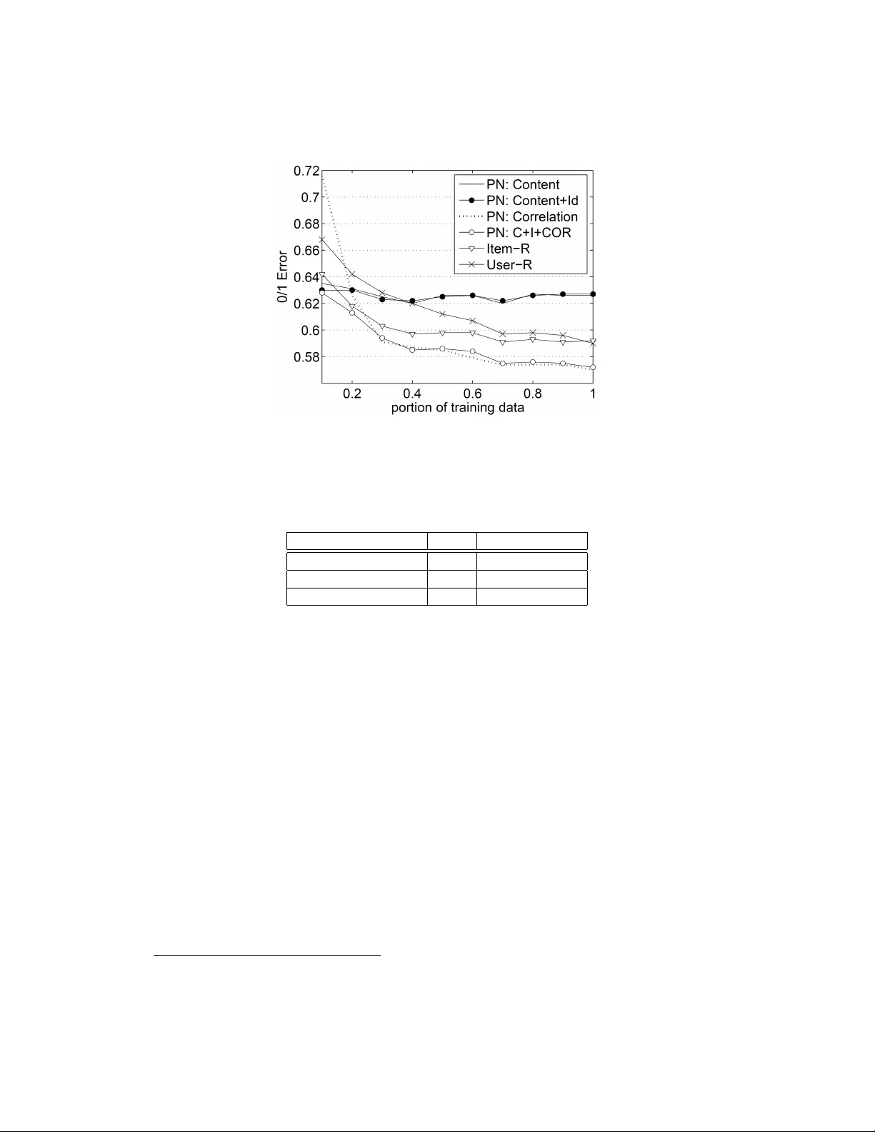
Preference Networks: Probabilistic Models for Recommendation Systems T ran The T ruyen, Dinh Q. Phung and Svetha V enkatesh Department of Computing, Curtin Uni versity of T echnology GPO Box U 1987, Perth, W A, Australia Abstract Recommender systems are important to help users select relev ant and personalised informa- tion ov er massiv e amounts of data av ailable. W e propose an unified framework called Preference Network (PN) that jointly models various types of domain knowledge for the task of recommen- dation. The PN is a probabilistic model that systematically combines both content-based filtering and collaborativ e filtering into a single conditional Markov random field. Once estimated, it serves as a probabilistic database that supports various useful queries such as rating prediction and top- N recommendation. T o handle the challenging problem of learning large networks of users and items, we employ a simple but ef fectiv e pseudo-likelihood with regularisation. Experi- ments on the movie rating data demonstrate the merits of the PN. K eywor ds: Hybrid Recommender Systems, Collaborativ e Filtering, Preference Networks, Condi- tional Markov Netw orks, Movie Rating. 1 Intr oduction W ith the explosi ve growth of the Internet, users are currently overloaded by massive amount of media, data and services. Thus selecti ve deliv ery that matches personal needs is very critical. Au- tomated recommender systems ha ve been designed for this purpose, and the y are deployed in major online stores such as Amazon [http://www .amazon.com], Netflix [http://www .netfix.com] and new services such as Google News [http://ne ws.google.com]. T wo most common tasks in recommender systems are predicting the score the user might give for a product (the rating pr ediction task ), and recommending a ranked list of most relev ant items (the top- N r ecommendation task ). The recommendations are made on the basis of the content of products and services ( content-based ), or based on collecti ve preferences of the cro wd ( collaborative filtering ), or both ( hybrid methods ). T ypically , content-based methods work by matching product attributes to user-profiles using classification techniques. Collaborative filtering, on the other hand, relies on preferences ov er a set products that a gi ven user and others have expressed. From the preferences, typically in term of numerical ratings, corr elation-based methods measure similarities between users (Resnick et al., 1994) (user-based methods) and products (Sarwar et al., 2001) (item- based methods). As content and preferences are complementary , hybrid methods often work best when both types of information is av ailable (Balabanovi ´ c and Shoham, 1997; Basu et al., 1998; Pazzani, 1999; Schein et al., 2002; Basilico and Hofmann, 2004). 1 Pr obabilistic modeling (Breese et al., 1998; Heckerman et al., 2001; Hofmann, 2004; Mar - lin, 2004) has been applied to the recommendation problem to some degree and their success has been mixed. Generally , they build probabilistic models that explain data. Earlier methods include Bayesian networks and dependency networks (Breese et al., 1998; Heckerman et al., 2001) have yet to prov e competitiv e against well-known correlation-based counterparts. The more recent work attempts to perform clustering. Some representativ e techniques are mixture models, probabilistic latent semantic analysis (pLSA) (Hofmann, 2004) and latent Dirichlet allocation (LD A) (Marlin, 2004). These methods are generative in the sense that it assumes some hidden process that gener- ates observed data such as items, users and ratings. The generati ve assumption is often made for algorithmic con venience and b ut it does not necessarily reflect the true process of the real data. Machine learning techniques (Billsus and Pazzani, 1998; Basu et al., 1998; Basilico and Hof- mann, 2004) address the rating prediction directly without making the generative assumption. Rather , they map the recommendation into a classification problem that existing classifiers can solve (Basu et al., 1998; Zhang and Iyengar, 2002). The map typically considers each user or each item as an independent problem, and ratings are training instances. Howe ver , the assumption that training in- stances are independently generated does not hold in collaborativ e filtering. Rather all the ratings are interconnected directly or indirectly through common users and items. T o sum up, it is desirable to b uild a recommendation system that can seamlessly integrate content and correlation information in a disciplined manner . At the same time, the system should address the prediction and recommendation tasks directly without replying on strong prior assumptions such as generativ e process and independence. T o that end, we propose a probabilistic graphical formula- tion called Preference Network (PN) that has these desirable properties. The PN is a graph whose verte xes represent ratings (or preferences) and edges represent dependencies between ratings. The networked ratings are treated as random variables of conditional Markov random fields (Lafferty et al., 2001). Thus the PN is a formal and e xpressiv e formulation that supports learning from existing data and various inference tasks to make future prediction and recommendation. The probabilistic dependencies between ratings capture the correlations between co-rating users (as used in (Resnick et al., 1994)) and between co-rated items (as used in (Sarwar et al., 2001)). Different from pre vious probabilistic models, the PN does not make any generativ e assumption. Rather , prediction of preferences is addressed directly based on the content and prior ratings av ail- able in the database. It also av oids the independence assumption made in the standard machine learning approach by supporting collective classification of preferences. The nature of graphical modeling enables PN to support missing ratings and joint predictions for a set of items and users. It provides some measure of confidence in each prediction made, making it easy to assess the na- ture of recommendation and rank results. More importantly , our experiments show that the PNs are competitiv e against the well-kno wn user-based method (Resnick et al., 1994) and the item-based method (Sarwar et al., 2001). 2 Recommender Systems This section provides some background on recommender systems and we refer readers to (Adomavi- cius and T uzhilin, 2005) for a more comprehensiv e survey . Let us start with some notations. Let U = { u 1 , . . . , u M } be the set of M users (e.g. service subscribers, movie vie wers, W ebsite visitors or product buyers), and I = { i 1 , . . . , i L } be the set of L products or items (e.g. services, movies, W ebpages or books) that the user can select from. Let us further denote M = { r ui } the prefer ence matrix where u is the user inde x, i is the item inde x, and r ui is the preference or the numerical rating 4 3 5 5 4 5 3 4 3 2 3 5 1 4 2 3 4 5 1 2 3 4 5 6 7 8 item user 1 2 3 4 5 6 7 8 5 4 5 3 4 3 5 4 5 4 5 4 5 Figure 1: Preference matrix. Entries are numerical rating (or preference) and empty cells are to be filled by the recommender system. of user u ov er item i (see Figure 1 for an illustration). In this paper , we assume that ratings have been appropriately transformed into integers, i.e. r ui ∈ { 1 , 2 , ..., S } . T ypically , a user usually rates only a small number of items and thus making the preference matrix M extremely sparse. For e xample, in the MovieLens dataset that we use in our experiments (Section 4), only about 6.3% entries in the M matrix are filled, and in large e-commerce sites, the sparsity can be as small as 0.001%. The rating prediction task in recommender systems can be considered as filling the empty cells in the preference matrix. Of course, due to the data sparsity , filling all the cells is impractical and often unnecessary because each user will be interested in a very small set of items. Rather , it is only appropriate for a limited set of entries in each ro w (corresponding to a user). Identifying the most relev ant entries and ranking them are the goal of top- N recommendation. Recommender techniques often fall into three groups: content-based , collabor ative filtering , and hybrid methods that combines the former two groups. Content-based methods rely on the content of items that match a user’ s profile to make recommen- dation using some classification techniques (e.g. see (Mooney and Roy, 2000)). The content of an item is often referred to the set of attrib utes that characterise it. For example, in movie recommenda- tion, item attributes include movie genres, release date, leading actor/actress, director , ratings by crit- ics, financial aspects, movie description and revie ws. Similarly , user attributes include static infor- mation such as age 1 , sex, location, language, occupation and marriage status and dynamic informa- tion such as watching time (day/night/late night), context of use (e.g. home/theater/family/dating/group/company), and in case of on-demand videos, what other TV channels are showing, what the person has been watching in the past hours, days or weeks. Collaborative filtering takes a dif ferent approach in that recommendation is based not only on 1 Strictly speaking, age is not truly static, but it changes really slo wly as long as selling is concerned. 8 7 5 4 5 3 4 3 5 4 5 4 5 4 5 4 3 5 5 4 5 3 4 3 2 3 5 1 4 2 3 4 5 1 2 3 4 5 6 7 8 item user 1 2 3 4 5 6 4 3 5 5 4 5 3 4 3 2 3 5 1 4 2 3 4 5 1 2 3 4 5 6 7 8 item user 1 2 3 4 5 6 7 8 5 4 5 3 4 3 5 4 5 4 5 4 5 (a) (b) Figure 2: User -based correlation (a) and Item-based correlation (b). the usage history of the user but also on experience and wisdom of related people in the user-item network. Most existing algorithms taking some measure of correlation between co-rating users or co-rated items. One family , known as user -based (sometimes memory-based) methods (Resnick et al., 1994), predicts a new rating of an item based on existing ratings on the same item by other users: r ui = ¯ r u + P v ∈ U ( i ) s ( u, v )( r ui − ¯ r v ) P v ∈ U ( i ) | s ( u, v ) | where s ( u, v ) is the similarity between user u and user v , U ( i ) is the set of all users who rate item i , and ¯ r u is the av erage rating by user u . The similarity s ( u, v ) is typically measured using Pearson’ s correlation: P i ∈ I ( u,v ) ( r ui − ¯ r u )( r v i − ¯ r v ) h P i ∈ I ( u,v ) ( r ui − ¯ r u ) 2 i 1 2 h P j ∈ I ( u,v ) ( r v j − ¯ r v ) 2 i 1 2 where I ( u, v ) is the set of all items co-rated by users u and v . See Figure 2a for illustration. This similarity is computed offline for e very pair of users who co-rate at least one common item. The main drawback of user-based methods is in its lack of ef ficiency at prediction time because each prediction require searching and summing over all users who rate the current item. The set of such users is often very large for popular items, sometimes including all users in the database. In contrast, each user typically rates only a very limited number of items. Item-based methods (Sarwar et al., 2001) exploit that fact by simply exchanging the role of user and item in the user- based approach. Similarity between items s ( i, j ) can be computed in se veral ways including the (adjusted) cosine between two item vectors, and the Pearson correlation. For example, the adjusted cosine similarity is computed as P u ∈ U ( i,j ) ( r ui − ¯ r u )( r uj − ¯ r u ) h P u ∈ U ( i,j ) ( r ui − ¯ r u ) 2 i 1 2 h P v ∈ U ( i,j ) ( r v j − ¯ r v ) 2 i 1 2 where U ( i, j ) is the set of all users who co-rate both items i and j . See Figure 2b for illustration. The new rating is predicted as r ui = ¯ r i + P j ∈ I ( u ) s ( i, j )( r uj − ¯ r j ) P j ∈ I ( u ) | s ( i, j ) | where I ( u ) is the set of items rated by user u . Many other methods attempt to build a model of training data that then use the model to per- form prediction on unseen data. One class of methods employ probabilistic graphical models such as Bayesian networks (Breese et al., 1998), dependency networks (Heckerman et al., 2001), and restricted Boltzmann machines (Salakhutdinov et al., 2007). Our proposed method using Markov networks f all under the cate gory of undirected graphical models. It resembles dependenc y networks in the way that pseudo-likelihood (Besag, 1974) learning is employed, but dependency networks are generally inconsistent probabilistic models. In (Salakhutdinov et al., 2007), the authors build a generativ e Boltzmann machine for each user with hidden variables, while our method constructs a single discriminativ e Markov netw ork for the whole database of all ratings. Much of other probabilistic work attempts to perform clustering. This is an important technique for reducing the dimensionality and noise, dealing with data sparsity and more significantly , dis- cov ering latent structures. Here the latent structures are either communities of users with similar tastes or cate gories of items with similar features. Some representativ e techniques are mixture mod- els, probabilistic latent semantic analysis (pLSA) (Hofmann, 2004) and latent Dirichlet allocation (LD A) (Marlin, 2004). These methods try to uncover some hidden process which is assumed to generate items, users and ratings. In our approach, no such generation is assumed and ratings are modeled conditionally giv en items and users and prior knowledge. Statistical machine learning techniques (Billsus and Pazzani, 1998; Basu et al., 1998; Zhang and Iyengar, 2002; Basilico and Hofmann, 2004; Zitnick and Kanade, 2004) have also been used to some extent. One of the ke y observations made is that there is some similarity between text classification and rating prediction (Zhang and Iyengar, 2002). Howe ver , the main dif ficulty is that the features in collaborati ve filtering are not rich and the nature of prediction is different. There are two ways to conv ert collaborative filtering into a classification problem (Billsus and Pazzani, 1998). The first is to build a model for each item, and ratings by different users are treated as training instances. The other builds a model for each user, and ratings on dif ferent items by this user are considered as training instances (Breese et al., 1998). These treatments, howe ver , are complementary , and thus, there should be a better way to systematically unify them (Basu et al., 1998; Basilico and Hofmann, 2004). That is, the pairs (user ,item) are now as independent training instances. Our approach, on the other hand, considers the pair as just a node in the network, thus relaxing the independence assump- tion. Hybrid methods exploit the fact that content-based and collaborative filtering methods are com- plementary (Balabanovi ´ c and Shoham, 1997; Basu et al., 1998; Pazzani, 1999; Schein et al., 2002; Basilico and Hofmann, 2004). For example, the content-based methods do not suffer from the so- called cold-start problem (Schein et al., 2002) in standard collaborative filtering. The situation is when new user and new item are introduced to the database, as no previous ratings are av ailable, purely correlation-based methods cannot work. On the other hand, content information av ailable is sometimes very limited to basic attributes that are shared by many items or users. Prediction by pure content-based methods in that case cannot be personalised and may be inaccurate. Some work approaches the problem by making independent predictions separately using a content-based method and a collaborative filtering method and then combining the results (Claypool et al., 1999). Others (e.g. (Basilico and Hofmann, 2004)) create joint representation of content and collaborativ e features. W e follow the latter approach. 3 Pr eference Networks f or Hybrid Recommendation 3.1 Model Description Let us start with the preference matrix M = { r ui } discussed pre viously (cf. Sec. 2), where we treat each entry r ui in M as a random variable, and thus ideally we would be interested in a single joint model over K M variables for both the learning phase and the prediction/recommendation phase. Howe ver , in practice, K M is extremely large (e.g., 10 6 × 10 6 ) making computation intractable. In addition, such a modeling is unncessary , because, as we have mentioned earlier in Section 2, a user is often interested in a moderate number of items. As a result, we adopt a two-step strategy . During the learning phase, we limit to model the joint distribution over existing ratings. And then during the prediction/recommendation phase, we extend the model to incoporate to-be-predicted entries. Figure 3: A fragment of the Preference Network. W e b uild the model by first representing the ratings and their relations using an undirected graph and then defining a joint distrib ution ov er the graph. Denote by G = ( V , E ) an undirected graph that has a set of vertex es V and a set of edges E . Each verte x in V in this case represents a rating r ui of user u over item i and each edge in E capture a relation between two ratings. The set E defines a topological structure for the network, and specify ho w ratings are related. W e define the edges as follows. There is an edge between any two ratings by the same user , and an edge between two ratings on the same item. As a result, a verte x of r ui will be connected with U ( i ) + I ( u ) − 2 other vertices. Thus, for each user , there is a fully connected subnetwork of all ratings she has made, plus connections to ratings by other users on these items. Likewise, for each item, there is a fully connected subnetwork of all ratings by different users on this item, plus connections to ratings on other items by these users. The resulting network G is typically very densely connected because U ( i ) can be potentially very lar ge (e.g. 10 6 ). Let us now specify the probabilistic modeling of the ratings and their relations that respect the graph G . Denote t = ( u, i ) and let T = { t } be the set of a pair inde x (user , item), which corresponds to entries used in each phase. For notation conv enience let X = { r ui | ( u, i ) ∈ T } denote the joint set of all variables, and the term ‘preference’ and ‘rating’ will be used exchangeably . When there is no confusion, we use r u to denote ratings related to user u and r i denotes ratings related to item i . In our approach to the hybrid recommendation task, we consider attributes of items { a i } L i =1 , and attributes of users { a u } M i = u . Let o = {{ a i } L i =1 , { a u } M i = u } , we are interested in modeling the conditional distribution P ( X | o ) of all user ratings X giv en o . W e employ the conditional Marko v random field (Lafferty et al., 2001) as the underlying inference machinery . As X collectiv ely repre- sents users’ preferences, we refer this model as Pr efer ence Network . Preference Network (PN) is thus a conditional Markov random field that defines a distribution P ( X | o ) o ver the graph G : P ( X | o ) = 1 Z ( o ) Ψ( X, o ) , where Ψ( X, o ) = Y t ∈V ψ t ( r t , o ) Y ( t,t 0 ) ∈E ψ t,t 0 ( r t , r t 0 , o ) (1) where Z ( o ) is the normalisation constant to ensure that P X P ( X | o ) = 1 , and ψ ( . ) is a positiv e function, often known as potential . More specifically , ψ t ( r t , o ) encodes the content information associated with the rating r t including the attributes of the user and the item. On the other hand, ψ t,t 0 ( r t , r t 0 , o ) captures the correlations between two ratings r t and r t 0 . Essentially , when there are no correlation potentials, the model is purely content-based, and when there are no content poten- tials, the model is purely collborative-filtering. Thus the PN integrates both types of recommendation in a seamlessly unified framew ork. The contrib ution of content and correlation potentials to the joint distribution will be adjusted by weighting parameters associated with them. Specifically , the parameters are encoded in potentials as follows ψ t ( r t , o ) = exp  w > v f v ( r t , o )  (2) ψ t,t 0 ( r t , r t 0 , o ) = exp  w > e f e ( r t , r t 0 , o )  (3) where f ( . ) is the feature vector and w is the corresponding weight vector . Thus together with their weights, the features realise the contribution of the content and the strength of correlations between items and users. The design of features will be elaborated further in Section 3.2. Parameter estimation is described in Section 3.3. 3.2 F eature Design and Selection Corresponding to the potentials in Equations 2 and 3, there are attribute-based features and correlation- based features. Attrib ute-based features include user/item identities and contents. Identity Featur es . Assume that the ratings are integer , ranging from 1 to S . W e know from the database the av erage rating ¯ r i of item i which roughly indicates the general quality of the item with respect to those who hav e rated it. Similarly , the a verage rating ¯ r u by user u over items she has rated roughly indicates the user-specific scale of the rating because the same rating of 4 may mean ‘OK’ for a regular user , but may mean ‘excellent’ for a critic. W e use two features item-specific f i ( r ui , i ) and user-specific f u ( r ui , u ) : f i ( r ui , i ) = g ( | r ui − ¯ r i | ) , f u ( r ui , u ) = g ( | r ui − ¯ r u | ) where g ( α ) = 1 − α/ ( S − 1) is used to ensure that the feature values is normalized to [0 , 1] , and when α plays the role of rating de viation, g ( α ) = 1 for α = 0 . Content Featur es . For each rating by user u on item i , we hav e a set of item attributes a i and set of user attrib utes a u . Mapping from item attributes to user preference can be carried out through the following feature f u ( r ui ) = a i g ( | r ui − ¯ r u | ) Similarly , we are also interested in seeing the classes of users who like a given item through the following mapping f i ( r ui ) = a u g ( | r ui − ¯ r i | ) Correlation F eatures . W e design two features to capture correlations between items or users. Specifically , the item-item f i,j ( · ) features capture the fact that if a user rates two items then after offsetting the goodness of each item, the ratings may be similar f i,j ( r ui , r uj ) = g ( | ( r ui − ¯ r i ) − ( r uj − ¯ r j ) | ) Like wise, the user -user f u,v ( · ) features capture the idea that if two users rate the same item then the ratings, after offset by user’ s own scale, should be similar: f u,v ( r ui , r v i ) = g ( | ( r ui − ¯ r u ) − ( r v i − ¯ r v ) | ) Since the number of correlation features can be large, making model estimation less rob ust, we select only item-item features with positiv e correlation (giv en in Equation 1), and user-user features with positiv e correlations (giv en in Equation 1). 3.3 Parameter Estimation Since the network is densely connected, learning methods based on the standard log-likelihood log P ( X | o ) are not applicable. This is because underlying inference for computing the log-likelihood and its gradient is only tractable for simple networks with simple chain or tree structures (Pearl, 1988). As a result, we resort to the simple but effecti ve pseudo-likelihood learning method (Besag, 1974). Specifically , we replace the log likelihood by the regularised sum of log local likelihoods L ( w ) = X ( u,i ) ∈T log P ( r ui |N ( u, i ) , o ) − 1 2 ¯ w > ¯ w (4) where, N ( u, i ) is the set of neighbour ratings that are connected to r ui . As we mentioned earlier , the size of the neighbourhood is |N ( u, i ) | = U ( i ) + I ( u ) − 2 . In the second term in the RHS, ¯ w = w / σ (element-wise division, regularised by a prior diagonal Gaussian of mean 0 and standard deviation vector σ ). Finally , the parameters are estimated by maximising the pseudo-likelihood ˆ w = arg max w L ( w ) (5) Not only is this regularised pseudo-likelihood simple to implement, it makes sense since the local conditional distribution P ( r ui |N ( u, i ) , o ) is used in prediction (Equation 7). W e limit ourselves to supervised learning in that all the ratings { r ui } in the training data are known. Thus, L ( w ) is a concav e function of w , and thus has a unique maximum. T o optimise the parameters, we use a simple stochastic gradient ascent procedure that updates the parameters after passing through a set of ratings by each user: w u ← w u + λ ∇L ( w u ) (6) where w u is the subset of parameters that are associated with ratings by user u , and λ > 0 is the learning rate. T ypically , 2-3 passes through the entire data are often enough in our experiments. Further details of the computation are included in Appendix A. 3.4 Prefer ence Prediction Recall from Section 3.1 that we employ a two-step modeling. In the learning phase (Section 3.3), the model includes all previous ratings. Once the model has been estimated, we extend the graph structure to include new ratings that need to be predicted or recommended. Since the number of ratings newly added is typically small compared to the size of existing ratings, it can be assumed that the model parameters do not change. The prediction of the rating r ui for user u ov er item i is giv en as ˆ r ui = arg max r ui P ( r ui | N ( u, i ) , o ) (7) The probability P ( ˆ r ui |N ( r ui ) , o ) is the measure of the confidence or ranking level in making this prediction. This can be useful in practical situations when we need high precision, that is, only ratings with the confidence abov e a certain threshold are presented to the users. W e can jointly infer the ratings r u of giv en user u on a subset of items i = ( i 1 , i 2 , .. ) as follo ws ˆ r u = arg max r u P ( r u | N ( u ) , o ) (8) where N ( u ) is the set of all existing ratings that share the common cliques with ratings by user u . In another scenario, we may want to recommend a relativ ely new item i to a set of promising users, we can make joint predictions r i as follows ˆ r i = arg max r i P ( r i | N ( i ) , o ) (9) where N ( i ) is the set of all existing ratings that share the common cliques with ratings of item i . It may appear non-obvious that a prediction may depend on unknown ratings (other predictions to be made) but this is the advantage of the Markov networks. Howe ver , joint predictions for a user are only possible if the subset of items is small (e.g. less than 20) because we have a completely connected subnetwork for this user . This is ev en worse for joint prediction of an item because the target set of users is usually v ery large. 3.5 T op- N recommendation In order to provide a list of top- N items to a gi ven user, the first step is usually to identify a candidate set of C promising items, where C ≥ N . Then in the second step, we rank and choose the best N items from this candidate set according to some measure of relev ance. Identifying the candicate set . This step should be as efficient as possible and C should be relatively small compared to the num- ber of items in the database. There are two common techniques used in user-based and item-based methods, respectively . In the user-based technique, first we idenfify a set of K most similar users, and then take the union of all items co-rated by these K users. Then we remove items that the user has pre viously rated. In the item-based technique (Deshpande and Karypis, 2004), for each item the user has rated, we select the K best similar items that the user has not rated. Then we take the union of all of these similar items. Indeed, if K → ∞ , or equi valently , we use all similar users and items in the database, then the item sets returned by the item-based and user-based techniques are identical . T o see why , we show that every candidate j returned by the item-based technique is also the candidate by the user-based techqnique, and vice versa. Recall that a pair of items is said to be similar if they are jointly rated by the same user . Let I ( u ) be the set of items rated by the current user u . So for each item j / ∈ I ( u ) similar to item i ∈ I ( u ) , there must exist a user v 6 = u so that i, j ∈ I ( v ) . Since u and v jointly rate i , they are similar users, which mean that j is also in the candidate set of the user -based method. Analogously , for each candidate j rated by user v , who is similar to u , and j / ∈ I ( u ) , there must be an item i 6 = j jointly rated by both u and v . Thus i, j ∈ I ( v ) , and therefore they are similar . This means that j must be a candidate by the item-based technique. In our Preference Networks, the similarity measure is replaced by the correlation between users or between items. The correlation is in turn captured by the corresponding correlation parameters. Thus, we can use either the user -user correlation or item-item correlation to identify the candicate set. Furthermore, we can also use both the correlation types and take the union of the two candidate sets. Ranking the candidate set . The second step in the top- N recommendation is to rank these C candicates according to some scoring methods. Ranking in the user-based methods is often based on item popularity , i.e. the number of users in the neighbourhood who hav e rated the item. Ranking in the item-based methods (Deshpande and Karypis, 2004) is computed by considering not only the number of raters but the similarity between the items being ranked and the set of items already rated by the user . Under our Preference Networks formulation, we propose to compute the change in system en- ergy and use it as ranking measure. Our PN can be thought as a stochastic physical system whose energy is related to the conditional distrib ution as follows P ( X | o ) = 1 Z ( o ) exp( − E ( X , o )) (10) where E ( X, o ) = − log Ψ( X, o ) is the system energy . Thus the lower energy the system state X has, the more probable the system is in that state. Let t = ( u, i ) , from Equations 2 and 3, we can see that the system energy is the sum of node-based ener gy and interaction energy E ( X , o ) = X t ∈V E ( r t , o ) + X ( t,t 0 ) ∈E E ( r t , r t 0 o ) where E ( r t , o ) = − w > v f v ( r t , o ) (11) E ( r t , r t 0 , o ) = − w > e f e ( r t , r t 0 , o ) (12) Recommending a new item i to a giv en user u is equi valent to extending the system by adding new rating node r ui . The change in system energy is therefore the sum of node-based energy of the new node, and the interation ener gy between the node and its neighbours. ∆ E ( r t , o ) = E ( r t , o ) + X t 0 ∈N ( t ) E ( r t , r t 0 , o ) For simplicity , we assume that the state of the existing system does not change after node addition. T ypically , we want the extended system to be in the most probable state, or equiv alently the system state with lo west energy . This means that the node that causes the most reduction of system energy will be prefered. Since we do not kno w the correct state r t of the ne w node t , we may guess by predicting ˆ r t using Equation 7. Let us call the energy reduction by this method the maximal ener gy change . Alternatively , we may compute the expected ener gy change to account for the uncertainty in the preference prediction E [∆ E ( r t , o )] = X r t P ( r t |N ( t ) , o )∆ E ( r t , o ) (13) 4 Experiments In this section, we ev aluate our Preference Network against well-established correlation methods on the movie recommendation tasks, which include rate prediction and top- N item recommendation. 4.1 Data and Experimental Setup W e use the MovieLens data 2 , collected by the GroupLens Research Project at the University of Minnesota from September 19th, 1997 through April 22nd, 1998. W e use the dataset of 100,000 ratings in the 1-5 scale. This has 943 users and 1682 movies. The data is divided into a training set of 80,000 ratings, and the test set of 20,000 ratings. The training data accounts for 852,848 and 411,546 user-based item-based correlation features. W e transform the content attributes into a v ector of binary indicators. Some attrib utes such as se x are categorical and thus are dimensions in the vector . Age requires some segmentation into intervals: under 18, 18-24, 25-34, 35-44, 45-49, 50-55, and 56+. W e limit user attributes to age, sex and 20 job categories 3 , and item attributes to 19 film genres 4 . Much richer movie content can be obtained from the Internet Movie Database (IMDB) 5 . 4.2 Accuracy of Rating Prediction In the training phrase, we set the learning rate λ = 0 . 001 and the regularisation term σ = 1 . W e compare our method with well-known user-based (Resnick et al., 1994) and item-based (Sarwar et al., 2001) techniques (see Section 2). T wo metrics are used: the mean absolute error (MAE) X ( u,i ) ∈T 0 | ˆ r ui − r ui | / ( |T 0 | ) (14) 2 http://www .grouplens.org 3 Job list: administrator, artist, doctor , educator , engineer , entertainment, executi ve, healthcare, homemaker , la wyer, librar- ian, marketing, none, other , programmer , retired, salesman, scientist, student, technician, writer . 4 Film genres: unknown, action, adventure, animation, children, comedy , crime, documentary , drama, fantasy , film-noir , horror , musical, mystery , romance, sci-fi, thriller , war , western. 5 http://us.imdb .com where T 0 is the set of rating index es in the test data, and the mean 0/1 error X ( u,i ) ∈T 0 δ ( ˆ r ui 6 = r ui ) / ( |T 0 | ) (15) In general, the MAE is more desirable than the 0/1 error because making exact prediction may not be required and making ‘closed enough’ predictions is still helpful. As item-based and user-used algorithms output real ratings, we round the numbers before computing the errors. Results sho wn in Figure 4 demonstrate that the PN outperforms both the item-based and user-based methods. Sensitivity to Data Sparsity . T o ev aluate methods against data sparsity , we randomly subsample the training set, but fix the test set. W e report the performance of different methods using the MAE metric in Figure 5 and using the mean 0/1 errors in Figure 6. As e xpected, the purely content-based method deals with the sparsity in the user-item rating matrix very well, i.e. when the training data is limited. Howe ver , as the content we use here is limited to a basic set of attributes, more data does not help the content-based method further . The correlation-based method (purely collaborati ve filtering), on the other hand, suffers sev erely from the sparsity , but outperforms all other methods when the data is sufficient. Finally , the hybrid method, which combines all the content, identity and correlation features, improv es the performance of all the component methods, both when data is sparse, and when it is sufficient. Figure 4: The mean absolute error of recommendation methods (Item: item-based method, and Item-R: item-based method with rounding). 4.3 T op- N Recommendation W e produce a ranked list of items for each user in the test set so that these items do not appear in the training set. When a recommended item is in the test set of a user, we call it is a hit. For ev aluation, we employ two measures. The first is the expected utility of the ranked list (Breese et al., 1998), and the second is the MAE computed ov er the hits. The expected utility takes into account of the Figure 5: The mean absolute error (MAE) of recommendation methods with respect to training size of the MovieLens data. (Item: item-based method, and Item-R: item-based method with rounding, User: user-based method, User-R: user-based method with rounding, Content: PNs with content- based features, C+I+CORR: PNs with content, identity and correlation features). position j of the hit in the list for each user u R u = X j 1 2 ( j − 1) / ( α − 1) (16) where α is the vie wing halflife. Follo wing (Breese et al., 1998), we set α = 5 . Finally , the expected utility for all users in the test set is giv en as R = 100 P u R u P u R max u (17) where R max u is computed as R max u = X j ∈ I 0 ( u ) 1 2 ( j − 1) / ( α − 1) (18) where I 0 ( u ) is the set of items of user u in the test set. For comparison, we implement a user-based recommendation in that for each user , we choose 100 best (positi vely) correlated users and then rank the item based on the number of times it is rated by them. T able 1 reports results of Preference Network with ranking measure of maximal energy change and expected ener gy change in producing the top 20 item recommendations. W e vary the rate of recall by varying the v alue of N , i.e. the recall rate typically improves as N increases. W e are interested in how the e xpected utility and the MAE changes as a function of recall. The expected energy change is used as the ranking criteria for the Preference Network. Figure 7 shows that the utility increases as a function of recall rate and reaches a saturation lev el at some point. Figure 8 exhibits a similar trend. It supports the argument that when the recall rate is smaller (i.e. N is small), we ha ve more confidence on the recommendation. For both measures, it is e vident that the Preference Network has an adv antage over the user -based method. Figure 6: The mean 0/1 error of recommendation methods with respect to training size of the Movie- Lens data. (Item: item-based method, and Item-R: item-based method with rounding, User: user- based method, User-R: user-based method with rounding, Content: PNs with content-based features, C+I+CORR: Ns with content, identity and correlation features). Method MAE Expected Utility User-based 0.669 46.61 PN (maximal energy) 0.603 47.43 PN (expected ener gy) 0.607 48.49 T able 1: Performance of top-20 recommendation. PN = Preference Network. 5 Discussion and Conclusions W e hav e presented a novel hybrid recommendation framew ork called Preference Networks that in- tegrates different sources of content (content-based filtering) and user’ s preferences (collaborativ e filtering) into a single network, combining advantages of both approaches, whilst ov ercoming short- comings of individual approaches such as the cold-start problem of the collaborati ve filtering. Our framew ork, based on the conditional Marko v random fields, are formal to characterise and amenable to inference. Our experiments show that PNs are competitiv e against both the well-known item- based and user-based collaborati ve filtering methods in the rating prediction task, and against the user-based method in the top- N recommendation task. Once learned, the PN is a probabilistic database that allo ws interesting queries. For example, the set of most influential items for a particular demographic user group can be identified based on the corresponding energies. Moreover , the conditional nature of the PN supports fusion of v arieties of information into the model through weighted feature functions. For example, the features can capture the assertion that if two people are friends, they are more likely to hav e similar tastes ev en though they ha ve not explicitly pro vided any common preferences 6 . 6 Friends are a influential factor of consumer behaviour via the ‘w ord-of-mouth’ process Figure 7: Expected utility as a function of recall. The larger utility , the better . PN = Preference Network. Finally , one main drawback the PNs inherit from the user-based methods is that it may be ex- pensiv e at prediction time, because it takes into account all users who are related to the current one. On-going work will in vestigate clustering techniques to reduce the number of pair -wise connections between users. A Marko v Property and Lear ning Log-linear Models This paper e xploits an important aspect of Markov networks known as Markov property that greatly simplifies the computation. Basically , the property ensures the conditional independence of a v ari- able r t with respect to other variables in the netw ork giv en its neighbourhood P ( r t | x \ r t , o ) = P ( r t |N ( t ) , o ) (19) where N ( t ) is the neighbourhood of r t . This explains why we just need to include the neighbour- hood in the Equation 7. This is important because P ( r t |N ( t ) , o ) can be easily ev aluated P ( r t |N ( t ) , o ) = 1 Z t ψ t ( r t , o ) Y t 0 ∈N ( t ) ψ t,t 0 ( r t , r t 0 , o ) where Z t = P r t ψ t ( r t , o ) Q t 0 ∈N ( t ) ψ t,t 0 ( r t , r t 0 , o ) . The parameter update rule in Equation 6 requires the computation of the gradient of the reg- ularised log pseudo-likelihood in Equation 4, and thus, the gradient of the log pseudo-likelihood Figure 8: MAE as a function of recall. The smaller MAE, the better . PN = Preference Network. L = log P ( r t |N ( t ) , o ) . Given the log-linear parameterisation in Equations 2 and 3, we ha ve ∂ log L ∂ w v = f v ( r t , o ) − X r 0 t P ( r 0 t |N ( t ) , o ) f v ( r 0 t , o ) ∂ log L ∂ w e = f e ( r t , r 0 t , o ) − X r 0 t P ( r 0 t |N ( t ) , o ) f e ( r 0 t , r t 0 , o ) Refer ences Adomavicius, G. and T uzhilin, A. (2005), ‘T o ward the next generation of recommender systems: a surve y of the state-of-the-art and possible extensions’, Knowledge and Data Engineering, IEEE T r ansactions on 17 (6), 734–749. Balabanovi ´ c, M. and Shoham, Y . (1997), ‘F ab: content-based, collaborativ e recommendation’, Com- munications of the A CM 40 (3), 66–72. Basilico, J. and Hofmann, T . (2004), ‘Unifying collaborativ e and content-based filtering’, Pr oceed- ings of the twenty-first international confer ence on Machine learning . Basu, C., Hirsh, H. and Cohen, W . (1998), ‘Recommendation as classification: Using social and content-based information in recommendation’, Pr oceedings of the Fifteenth National Conference on Artificial Intelligence . Besag, J. (1974), ‘Spatial interaction and the statistical analysis of lattice systems (with discus- sions)’, Journal of the Royal Statistical Society Series B 36 , 192–236. Billsus, D. and Pazzani, M. (1998), ‘Learning collaborative information filters’, Pr oceedings of the F ifteenth International Confer ence on Machine Learning pp. 46–54. Breese, J., Heckerman, D., Kadie, C. et al. (1998), ‘Empirical analysis of predictive algorithms for collaborati ve filtering’, Pr oceedings of the F ourteenth Confer ence on Uncertainty in Artificial Intelligence 461 . Claypool, M., Gokhale, A., Miranda, T ., Murnikov , P ., Netes, D. and Sartin, M. (1999), ‘Combin- ing content-based and collaborativ e filters in an online newspaper’, ACM SIGIR W orkshop on Recommender Systems . Deshpande, M. and Karypis, G. (2004), ‘Item-based top-N recommendation algorithms’, ACM T r ansactions on Information Systems (TOIS) 22 (1), 143–177. Heckerman, D., Chickering, D., Meek, C., Rounthwaite, R. and Kadie, C. (2001), ‘Dependency networks for inference, collaborativ e filtering, and data visualization’, The Journal of Machine Learning Resear ch 1 , 49–75. Hofmann, T . (2004), ‘Latent semantic models for collaborative filtering’, A CM T ransactions on Information Systems (TOIS) 22 (1), 89–115. Lafferty , J., McCallum, A. and Pereira, F . (2001), Conditional Random Fields: Probabilistic Models for Segmenting and Labeling Sequence Data, in ‘ICML ’, pp. 282–289. Marlin, B. (2004), ‘Modeling user rating profiles for collaborative filtering’, Advances in Neural Information Pr ocessing Systems 16 , 627–634. Mooney , R. and Roy , L. (2000), ‘Content-based book recommending using learning for text catego- rization’, Pr oceedings of the fifth A CM confer ence on Digital libraries pp. 195–204. Pazzani, M. (1999), ‘A Framew ork for Collaborative, Content-Based and Demographic Filtering’, Artificial Intelligence Revie w 13 (5), 393–408. Pearl, J. (1988), Pr obabilistic r easoning in intelligent systems: networks of plausible inference , Morgan Kaufmann, San Francisco, CA. Resnick, P ., Iacovou, N., Suchak, M., Bergstorm, P . and Riedl, J. (1994), GroupLens: An Open Architecture for Collaborativ e Filtering of Netne ws, in ‘Proceedings of ACM 1994 Conference on Computer Supported Cooperativ e W ork’, A CM, Chapel Hill, North Carolina, pp. 175–186. Salakhutdinov , R., Mnih, A. and Hinton, G. (2007), Restricted Boltzmann machines for collaborati ve filtering, in ‘ICML ’. Sarwar , B., Karypis, G., Konstan, J. and Reidl, J. (2001), ‘Item-based collaborative filtering rec- ommendation algorithms’, Proceedings of the 10th international confer ence on W orld W ide W eb pp. 285–295. Schein, A., Popescul, A., Ungar , L. and Pennock, D. (2002), ‘Methods and metrics for cold-start recommendations’, Pr oceedings of the 25th annual international ACM SIGIR confer ence on Re- sear ch and development in information r etrie val pp. 253–260. Zhang, T . and Iyengar , V . (2002), ‘Recommender systems using linear classifiers’, Journal of Ma- chine Learning Resear ch 2 (3), 313–334. Zitnick, C. and Kanade, T . (2004), ‘Maximum entropy for collaborative filtering’, Pr oceedings of the 20th confer ence on Uncertainty in artificial intelligence pp. 636–643.