A path-integral approach to Bayesian inference for inverse problems using the semiclassical approximation

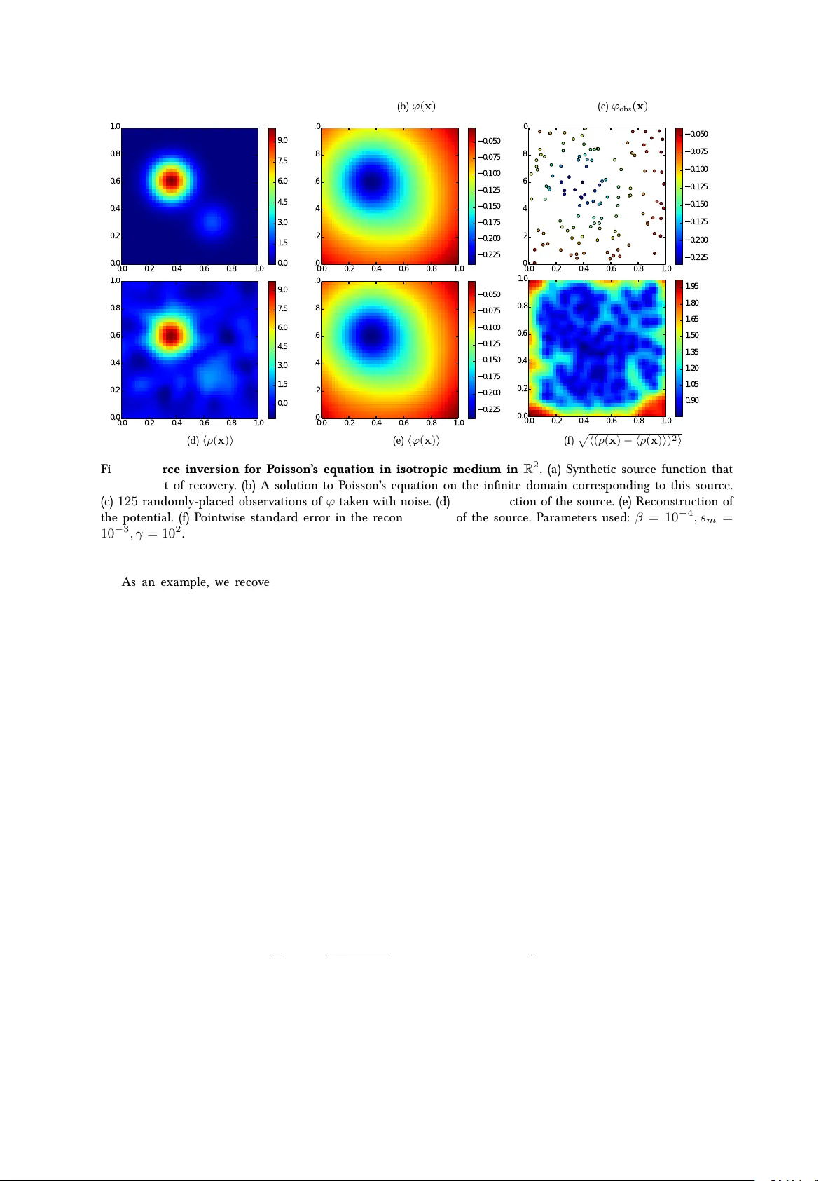
Journal o f Statistical Ph ysics manuscript No. (will be inserted by the editor) A path-int egral approach t o Ba y esian inf er ence f or in verse pr oblems using the semiclassical appr o ximation Joshua C. Chang · V an M. Sa vag e · T om Chou July 23, 2014 Abstract W e demonstrat e how pa th integrals oft en used in problems o f theoretical ph y sics can be adapted to pr o vide a machinery for perf orming Ba yesian inf er ence in f unction spaces. Such inf er ence comes about naturally in the study of in v erse pr oblems of r ecov ering continuous (in fi nite dimensional) coe ffi cient functions f r om ordinary or partial di ff er ential equations (ODE, PDE), a pr oblem which is typically ill-posed. Regularization of these problems using L 2 function spaces (Tikhonov regulariza tion) is equivalent to Ba yesian probabilistic infer ence, using a Gaussian prior . T he Ba y esian interpreta tion of inv erse pr oblem regularization is useful since it allow s one t o quantif y and characterize err or and degr ee of precision in the solution of inv erse pr oblems , as well as examine assumptions made in solving the problem – namely whether the subjective choice of regulariza tion is compatible with prior knowledg e. Using path-int egral formalism, Ba y esian infer ence can be explor ed thr ough various perturbative techniques, such as the semiclassical appro ximation, which we use in this manuscript. P erturbativ e path-int egral approaches, while o ff ering alterna tives to computational appr oaches like Mark ov -Chain-Monte-Carlo (MCMC), also pro vide natural starting points for MCMC methods that can be used t o r e fi ne appr oxima tions. In this manuscript, w e illustrat e a path-int egral formula tion for inv erse problems and demonstrat e it on an inv erse pr oblem in membrane biophysics as well as inv erse pr oblems in potential theories in volving the P oisson equation. K eywor ds Inv erse pr oblems · Ba y esian infer ence · F ield theor y · Path integral · P otential theory · Semiclassical appr oximation 1 Intr oduction One of the main conceptual challenges in solving inv erse pr oblems results from the fact that most int eresting inv erse pr oblems are not w ell-posed. One oft en chooses a solution that is “useful," or that optimizes some regularity criteria. Such a task is commonly kno wn as regular ization, of which there ar e many variants. One of the most commonly used methods is Tikhonov Regularization , or L 2 -penalized regularization [8, 9, 20, 32, 44]. Her e we fi rst demonstra te the concept behind Tikhono v regularization using one of the sim plest inv erse problems, the interpolation pr oblem. Tikhonov r egularization, when applied to interpolation, solv es the inv erse problem of J.C. Chang Mathematical Biosciences Institute,The Ohio State Univ ersity Jennings Hall, 3rd Floor, 1735 Neil A venue, Columbus , Ohio 43210 E-mail: chang.1166@mbi.osu.edu T . Chou UCLA Departments of Biomathematics and Mathema tics BO X 951766, Room 5309 Life Sciences, Los Angeles, C A 90095-1766 E-mail: tomchou@ucla.edu V .M. Sav age Santa F e Institute, Santa F e, NM 87501 UCLA Department of Biomathematics and Department of E cology and Ev olutionar y Biology BO X 951766, Room 5205 Life Sciences, Los Angeles, C A 90095-1766 E-mail: vsa vag e@ucla.edu constructing a continuous function ϕ : R d → R from point-wise measurements ϕ obs at positions { x m } by seeking minima with respect to a cost f unctional of the f orm H [ ϕ ] = 1 2 M X m =1 1 s 2 m ( ϕ ( x m ) − ϕ obs ( x m )) 2 | {z } H obs [ ϕ ] + 1 2 X α γ α Z | D α ϕ | 2 d x | {z } H reg [ ϕ ] , (1) wher e the constants 1 /s 2 m , γ α > 0 are w eighting parameters, and D α = Q d j =1 ( − i∂ x j ) α j is a di ff er ential operat or of order α = ( α 1 , . . . , α d ) . Assuming D α is isotropic and integ er -order ed, it is possible to inv oke integra tion-by -parts to writ e H [ ϕ ] in the quadratic form H [ ϕ ] = 1 2 M X m =1 1 s 2 m ( ϕ ( x m ) − ϕ obs ( x m )) 2 + 1 2 Z ϕ ( x ) P ( − ∆ ) ϕ ( x ) d x , (2) wher e P ( · ) is a polynomial of possibly in fi nite order , ∆ is the Laplacian operator , and we ha ve assumed that boundary terms vanish. In the r emainder of this wor k , we will focus on energy f unctionals of this form. This expr ession is known in previous litera ture as the Infor mation Hamiltonian [11]. Using this form of regularization ser v es two primar y pur poses. First, it selects smooth solutions to the inv erse pr oblem, with the amount of smoothness controlled by H reg . F or example, if only H obs is used, the solution can be any function that connects the obser vations ϕ obs at the measur ed points x j , such as a piecewise a ffi ne solution. Y et, such solutions ma y be phy sically unr easonable (not smooth). Second, it transforms the original inv erse pr oblem into a conv ex optimization problem that possesses an unique solution [3, 10]. If all of the coe ffi cients of P are non-nega tive, then the pseudo-di ff er ential-operat or P ( − ∆ ) is positiv e-de fi nite [22], guarant eeing uniqueness. These featur es of Tikhono v regularization make it attractiv e; ho we ver , one needs to mak e certain choices. In practical settings , one will need to chose both the degree of the di ff er ential operat or and value of the parameters γ α . T hese two choices adjust the trade-o ff between data agr eement and r egularity . 1.1 Ba yesian inv erse pr oblems The problem of parameter selection for regularization is well-addr essed in the conte xt of Bayesian infer ence, wher e r egularization paramet ers can be viewed pr obabilistically as prior -knowledg e of the solution. Ba yesian inf erence o v er continuous f unction spaces has been applied to inv erse problems in sev eral conte xts. One of the fi rst applications of Bay esian inf erence to inv erse problems was in the study of quantum inv erse problems [28], wher e it was noted that Gaussian priors could be used t o f ormulate fi eld theories. Subsequently , variants of this methodology hav e been used f or model reduction [29] and applied to many interpolation problems and inv erse pr oblems in fl uid mechanics [6, 19, 43], geology [13, 31, 38], cosmology [11, 34], and biology [18]. There is a wealth of literatur e concerning the computational aspects of Ba yesian inv erse problems. Many of these wor ks on inv erse problems are viewed through the framew ork and languag e of data assimilation through Mark ov Chain Monte Carlo approaches [4, 4, 37, 39, 40]. Appro ximation methods based on sparsity ha ve also been dev eloped [42]. Finally , there is a larg e body of w ork on the theoretical aspects of maximum aposteriori infer ence for Ba yesian inv erse problems including questions of exist ence of solutions and conv erg ence to solutions [7, 25–27, 43] 2 Field-theoretic formulation Ba yesian inf erence on ϕ entails the constr uction of a pr obability density π known as the poster ior distribution π ( ϕ ) which obeys Bayes’ r ule, π ( ϕ ) = likelihood z }| { Pr( ϕ obs | ϕ ) prior z }| { Pr( ϕ ) Z [0] (3) wher e Z [0] is the partition f unction or normalization factor . The posterior density π is a density in a space of functions. T he inv erse problem is then inv estigat ed by computing the statistics of the posterior probability density π ( φ ) thr ough the e valuation of Z [0] . T he solution of the in verse pr oblem corresponds t o the speci fi c ϕ that maximizes π ( φ ) , subject to prior kno wledg e encoded in the prior pr obability density Pr( ϕ ) . T his solution is known as the mean fi eld solution. The variance, or error , of the mean fi eld solution is f ound by computing the variance of the posterior distribution about the mean fi eld solution. 2 This view of in verse problems also leads naturally t o the use of functional integration and perturbation methods common in theoretical phy sics [24, 45]. Use of the pr obabilistic viewpoint allows for exploration of inv erse problems bey ond mean fi eld, with the chief advantag e of pro viding a method for uncertainty quanti fi cation. As shown in [13, 28], Tikhonov regulariza tion has the probabilistic interpr etation of Ba yesian infer ence with a Gaussian prior distribution. That is, the r egularization t erm in Eq 2 combines with the data term to specify a posterior distribution of the f orm π ( ϕ | ϕ obs ) = 1 Z [0] e − H [ ϕ ] = 1 Z [0] exp ( − M X m =1 1 s 2 m ( ϕ ( x m ) − ϕ obs ( x m )) 2 ) | {z } likelihood (exp {− H obs } ) exp  − 1 2 Z ϕ ( x ) P ( − ∆ ) ϕ ( x ) d x  | {z } prior (exp {− H reg } ) (4) wher e the partition function Z [0] = Z D ϕe − H [ ϕ ] = Z D ϕe − H reg [ ϕ ] | {z } d W [ ϕ ] e − H obs [ ϕ ] (5) is a sum ov er the contributions of all functions in the separable Hilbert space { ϕ : H reg [ ϕ ] < ∞} . This sum is expr essed as a path integral , which is an integral ov er a f unction space. The f ormalism for this type of integral came about fi rst from high-ener gy theoretical ph ysics [14], and then found application in nearly all ar eas of phy sics as well as in the repr esentation of both Mark ovian [5, 15, 35], and non-Mark ovian [16, 36] stochastic processes. In the case of Eq. 5, wher e the fi eld theor y is real-v alued and the operator P ( − ∆ ) is self-adjoint, a type of functional integral based on abstract W iener measure may be used [23]. The abstract W iener measure d W [ ϕ ] used for Eq. 5 subsumes the prior term H reg , and it is helpful t o think of it as a Gaussian measure ov er lattice points taken to the continuum limit. When the functional integral of the exponentiat ed energy f unctional can be written in the form Z [0] = Z D ϕ exp  − 1 2 Z Z ϕ ( x ) A ( x , x 0 ) ϕ ( x 0 ) d x d x 0 + Z b ( x ) ϕ ( x ) d x  , (6) then the probability density is Gaussian in function-space and the functional integral of Eq. 6 has the solution [45] Z [0] = exp  1 2 Z Z b ( x ) A − 1 ( x , x 0 ) b ( x 0 ) d x d x 0 − 1 2 log det A  . (7) The operat ors A ( x , x 0 ) and A − 1 ( x , x 0 ) are relat ed throug h the relationship Z A ( x , x 0 ) A − 1 ( x 0 , x 00 ) d x 0 = δ ( x − x 00 ) . (8) Upon neglecting H obs , the f unctional integral of Eq. 5 can be expressed in the form of Eq. 6 with A ( x , x 0 ) = P ( − ∆ ) δ ( x − x 0 ) . T he pseudo-di ff er ential-operator P ( − ∆ ) acts as an in fi nite-dimensional v ersion of the inv erse of a covariance matrix. It encodes the a-priori spatial correla tion, implying that values of the function ϕ are spatially corr elat ed according to a corr elation function (Gr een’ s function) A − 1 ( x , y ) = G ( x , y ) : R d × R d → R thr ough the r elationship implied by Eq. 8, P ( − ∆ ) G ( x , y ) = δ ( x − y ) so that G ( x , y ) =  1 2 π  d R R d e − i k · ( y − x ) 1 P ( | k | 2 ) d k where P ( | k | 2 ) is the symbol of the pseudo-di ff er ential-operat or P ( − ∆ ) . It is evident that w hen performing Tikhono v r eg- ularization, one should chose regulariza tion that is re fl ectiv e of prior know ledge of correlations, whenev er a vailable. 2.1 Mean fi eld inv erse problems W e turn now to the more-g eneral pr oblem, w her e one seeks r ecovery of a scalar function ξ given measur ements of a coupled scalar function ϕ ov er interior points x i , and the relationship between the measured and desired functions is given by a partial di ff er ential equation F ( ϕ ( x ) , ξ ( x )) = 0 x ∈ Ω \ ∂ Ω . (9) 3 As befor e, we regularize ξ using knowledg e of its spatial corr elation, and write a posterior probability density π [ ϕ, ξ | ϕ obs ] = δ ( F ( ϕ, ξ )) Z [0] exp ( − 1 2 Z M X m =1 δ ( x − x m ) ( ϕ ( x ) − ϕ obs ( x )) 2 s 2 m d x − 1 2 Z ξ ( x ) P ( − ∆ ) ξ ( x ) d x ) , wher e w e ha ve used the Dirac-delta function δ t o specify that our observations are taken with noise s 2 m at certain po- sitions x m , and an in fi nite-dimensional delta functional δ to specify that F ( ϕ, ξ ) = 0 ev erywhere. Using the inv erse F ourier -transformation, one can repr esent δ in path-integral form as δ ( F ( ϕ, ξ )) = R D λe − i R λ ( x ) F ( ϕ ( x ) ,ξ ( x )) d x , wher e λ ( x ) , is a F ourier wa ve vector . The reason for this notation will soon be clear . W e now ha ve a posterior pr obability distribution of three functions ϕ, ξ , λ of the form π [ ϕ, ξ , λ ( x ) | ϕ obs ] = 1 Z [0] exp {− H [ ϕ, ξ , λ ] } , (10) wher e the par tition f unctional is Z [0] = Z Z Z D ϕ D ξ D λ exp {− H [ ϕ, ξ , λ ] } , (11) and the Hamiltonian H [ ϕ, ξ , λ ; ϕ obs ] = 1 2 Z M X m =1 δ ( x − x m ) ( ϕ ( x ) − ϕ obs ( x )) 2 s 2 m d x + 1 2 Z ξ ( x ) P ( − ∆ ) ξ ( x ) d x + i Z λ ( x ) F ( ϕ, ξ ) d x , (12) is a f unctional of ϕ, ξ , and the F ourier wa v e vect or λ ( x ) . Similar Hamiltonians, pro viding a pr obabilistic model for data in the context of inv erse problems, hav e appeared in pre vious literatur e [11, 28, 43], w her e they ha v e been r eferr ed t o as Infor mation Hamiltonians . Maximization of the post erior pr obability distribution, also known as Ba y esian maximum a posteriori estima tion (MAP) infer ence, is performed by minimization of the corresponding energy functional (Eq. 12) with respect to the functions ϕ, ξ , λ . One ma y perform this infer ence by solving the associat ed Euler -Lagrange equations P ( − ∆ ) ξ + δ δ ξ ( x ) Z λ ( x ) F ( ϕ, ξ ) d x = 0 , (13) M X n =1 δ ( x − x n )( ϕ ( x ) − ϕ obs ( x )) + δ δ ϕ ( x ) Z λ ( x ) F ( ϕ, ξ ) d x = 0 (14) F ( ϕ, ξ ) = 0 , (15) wher e λ ( x ) here ser v es the r ole of a Lagrang e multiplier. Solving this system of partial di ff erential equations simul- taneously allows one to arrive at the solution to the original Tikhonov -regularized inv erse problem. Now , suppose one is interest ed in estimating the precision of the given solution. T he fi eld-theor etic formula tion of in verse problems pr ovides a wa y of doing so. 2.2 Bey ond mean- fi eld – semiclassical appr o ximation The functions ϕ, ξ , λ : R d → R each constitut e scalar fi elds 1 . Field theor y is the study of statistical properties of such fi elds throug h evalua tion of an associated path integ ral (functional integral). Field theor y applied to Ba yesian infer ence has appear ed in prior literatur e under the names Bay esian Field theor y [13, 28, 43], and Information Field Theor y [11]. In general, fi eld theor y deals with functional int egrals of the form Z [ J ] = Z D ϕ exp ( −  1 2 Z Z ϕ ( x ) A ( x , x 0 ) ϕ ( x 0 ) d x d x 0 + Z V [ ϕ ( x )] d x  | {z } H [ ϕ ] + Z J ( x ) ϕ ( x ) d x ) , (16) 1 W e will use Gr eek letters to denote fi elds 4 wher e the Hamilt onian of inter est is reco ver ed when the source J = 0 , and the potential f unction V is nonlinear in ϕ . Assuming that after non-dimensionalization, V [ ϕ ] is rela tively small in comparison to the other terms, one is then able to expand the last term in formal T a ylor series so that after completing the Gaussian part of the integral as in Eq. 7, Z [ J ] = Z D ϕ ( exp  − 1 2 Z Z ϕ ( x ) A ( x , x 0 ) ϕ ( x 0 ) d x d x 0 + Z J ( x ) ϕ ( x ) d x  | {z } Gaussian ×  1 − Z V [ ϕ ] d x + . . .  ) ∝ exp  − V  δ δ J  exp  1 2 Z Z J ( x ) A − 1 ( x , x 0 ) J ( x 0 ) d x d x 0  . (17) In this wa y , Z [ J ] can be expr essed in series form as moments of a Gaussian distribution. The integral is of inter est because one can use it to reco ver moments of the desir ed fi eld throug h functional di ff er entiation, * Y k ϕ ( x k ) + = 1 Z [0] Y k δ δ J ( x k ) Z [ J ]      J =0 . (18) This appr oach is known as the w eak -coupling approach [45]. F or this expansion to hold, how ev er, the ext ernal pot ential V must be small in size compar ed to the quadratic term. T his assumption is not generally valid during Tikhonov r egularization, as common rules of thumb dictate that the data fi delity and the regulariza tion term should be of similar order of magnitude [2, 41]. Another perturbativ e approach – the one that we will tak e in this manuscript – is to expand the Hamiltonian in a f unctional T a ylor series H [ ϕ ] = H [ ϕ ? ] + 1 2 Z Z δ 2 H [ ϕ ? ] δ ϕ ( x ) ϕ ( x 0 ) ( ϕ ( x ) − ϕ ? ( x ))( ϕ ( x 0 ) − ϕ ? ( x 0 )) d x d x 0 + . . . (19) about its extremal point ϕ ? . T o the second or der (as shown), the expansion is known as the semiclassical approxima- tion [17] which pro vides an appro ximat e Gaussian density for the fi eld ϕ . Corr ections to the semiclassical expansion can be ev aluated by continuing this expansion to higher orders, wher e evaluation of the f unctional integral can be aided by the use of F eynman diagrams [14]. 2.3 Monte-Car lo for re fi nement of appro ximations The Gaussian appr oxima tion is useful because Gaussian densities ar e easy t o sample. One ma y sam ple a random fi eld ϕ ( x ) f r om a Gaussian distribution with inv erse-cov ariance A ( x , x 0 ) by solving the stochastic di ff erential equation 1 2 Z A ( x , x 0 ) ϕ ( x 0 ) d x 0 = η ( x ) , (20) wher e η is the unit white noise process which has mean h η ( x ) i = 0 , and spatial corr elation  η ( x ) η ( x 0 )  = δ ( x − x 0 ) . W ith the ability t o sample f r om the appro ximating Gaussian distribution of Eq. 19, one ma y use Monte-Car lo simulation to sample from the tr ue distribution by weig hting the samples obtained from the Gaussian distribution. Such an approach is known as importance sampling [30], w her e samples ϕ i ar e given importance w eigh ts w i accor ding to the ratio w i = exp ( − H appro x + H true ) / P j w j . Statistics of ϕ ma y then be calculated using the w eight ed samples; for instance expectations can be appro ximated as h g ( ϕ ( x )) i ≈ P i w i g ( ϕ i ( x )) . Using this method, one can re fi ne the original estimates of the statistics of ϕ . 3 Examples 3.1 Interpolation of the height of a rigid membrane or plat e W e fi rst demonstrate the fi eld theor y for inv erse problems on an interpolation problem wher e one is able to determine the regularizing di ff er ential operator based on prior knowledg e. This example corresponds to the interpolation ex- ample mentioned in the Intr oduction. Consider the problem w here one is attempting t o identify in thr ee-dimensions 5 the position of a membrane. F or simplicity , we assume that one is inter ested in obtaining the position of the mem- brane only over a restrict ed spatial domain, wher e one can use the Monge paramet erization to r educe the problem to two-dimensions and de fi ne the heigh t of the membrane ϕ : R 2 → R . Suppose one is able t o measur e the membrane in certain spatial locations { x m } , but one seeks t o also interpolate the membrane in regions that are not observable. Phy sically , models for fl uctuations in membranes are w ell known, for instance the Helfrich free-energy [12] sugg ests that one should use a r egularizing di ff er ential operat or P ( − ∆ ) = β ( κ∆ 2 − σ ∆ ) β , σ, κ > 0 , (21) wher e σ and κ are the membrane tension and bending rigidity , respectiv ely . T he Hamiltonian associated with the Helfrich operat or is H [ ϕ ; ϕ obs ] = 1 2 Z M X m =1 δ ( x − x m ) s 2 m ( ϕ ( x ) − ϕ obs ( x )) 2 d x + 1 2 Z ϕ ( x ) P ( − ∆ ) ϕ ( x ) d x , (22) and the mean- fi eld solution f or ϕ corr esponds to the extremal point of the Hamiltonian, which is the solution of the corr esponding Euler -Lagrange equation δ H δ ϕ = M X m =1 δ ( x − x m ) s 2 m ( ϕ ( x ) − ϕ obs ( x )) + P ( − ∆ ) ϕ ( x ) = 0 . (23) T o g o bey ond mean- fi eld, one ma y compute statistics of the probability distribution Pr( ϕ ) ∝ e − H [ ϕ ] , using the g enerating functional which is expr essed as a functional integral Z [ J ] ∝ Z D ϕ exp ( − 1 2 Z Z ϕ ( x ) " δ ( x − x 0 ) M X m =1 δ ( x 0 − x m ) s 2 m + P ( − ∆ ) δ ( x − x 0 ) # | {z } A ( x , x 0 ) ϕ ( x 0 ) d x d x 0 + Z " M X m =1 ϕ obs ( x ) δ ( x − x m ) s 2 m + J ( x ) # ϕ ( x ) d x ) , (24) wher e w e ha ve completed the squar e. According to Eq. 7, Eq. 24 has the solution Z [ J ] ∝ exp ( 1 2 Z Z J ( x ) A − 1 ( x , x 0 ) J ( x 0 ) d x 0 d x + Z J ( x ) M X m =1 ϕ obs ( x m ) A − 1 ( x , x m ) s 2 m d x ) . (25) Throug h functional di ff er entiation of Eq. 25, Eq. 18 implies that the mean- fi eld solution is h ϕ ( x ) i = M X m =1 ϕ obs ( x m ) A − 1 ( x , x m ) s 2 m , (26) and variance in the solution is D ϕ ( x ) − h ϕ ( x ) i , ϕ ( x 0 ) −  ϕ ( x 0 )  E = A − 1 ( x , x 0 ) . (27) T o solv e for these quantities , we compute the operat or A − 1 , which accor ding to Eq. 8, satis fi es the partial di ff er ential equation M X m =1 δ ( x m − x ) s 2 m A − 1 ( x , x 00 ) + P ( − ∆ ) A − 1 ( x , x 00 ) = δ ( x − x 00 ) . (28) Using the Green ’ s function for P ( − ∆ ) , G ( x , x 0 ) = − 1 2 π β σ  log  | x − x 0 |  + K 0  r σ κ | x − x 0 |  , (29) we fi nd 6 A − 1 ( x , x 00 ) = known z }| { G ( x , x 00 ) − M X m =1 known z }| { G ( x , x m ) unknown z }| { A − 1 ( x m , x 00 ) s 2 m . (30) T o calculat e A − 1 ( x , x 0 ) , we need A − 1 ( x m , x 0 ) , for m ∈ { 1 , . . . , M } . Solving for each of these simultaneously yields the equation A − 1 ( x , x 0 ) = G ( x , x 0 ) − G s ( x ) ( I + Λ ) − 1 G ( x 0 ) , (31) wher e G s ( x ) ≡ h G ( x , x 1 ) s 2 1 , G ( x , x 2 ) s 2 2 , . . . , G ( x , x M ) s 2 M i , G ( x ) ≡ [ G ( x , x 1 ) , G ( x , x 2 ) , . . . , G ( x , x M )] , and Λ ij ≡ G ( x i , x j ) /s 2 i . 0 . 0 0 . 5 1 . 0 1 . 5 2 . 0 2 . 5 0 . 0 0 . 5 1 . 0 1 . 5 2 . 0 2 . 5 − 6 − 5 − 4 − 3 − 2 − 1 0 1 2 3 (a) ϕ ( x ) 0 . 0 0 . 5 1 . 0 1 . 5 2 . 0 2 . 5 0 . 0 0 . 5 1 . 0 1 . 5 2 . 0 2 . 5 − 6 − 5 − 4 − 3 − 2 − 1 0 1 2 (b) h ϕ ( x ) i 0 . 0 0 . 5 1 . 0 1 . 5 2 . 0 2 . 5 0 . 0 0 . 5 1 . 0 1 . 5 2 . 0 2 . 5 0 . 0 0 0 . 0 5 0 . 1 0 0 . 1 5 0 . 2 0 (c) p h ( ϕ ( x ) − h ϕ ( x ) i ) 2 i Fig. 1: Interpolation o f a membrane. (a) A simulat ed membrane underg oing thermal fl uctuations is the object of r econstruction. (b) Mean- fi eld reconstruction o f the membrane using 100 randomly-placed measurements with noise. (c) P ointwise standard error in the reconstruction of the membrane. P arameters used: σ = 10 − 2 , β = 10 3 , κ = 10 − 4 , s m = 10 − 2 . Fig. 1 shows an example of the use of the Helfrich free energy for int erpolation. A sample of a membrane under - g oing thermal fl uctuations was taken as the object of reco very . U niformly , 100 randomly-placed, noisy obser va tions of the height of the membrane wer e taken. The mean- fi eld solution f or the position of the membrane and the standard err or in the solution are present ed. The standard error is not uniform and dips to appro ximately the measurement err or at locations wher e measur ements wer e tak en. 3.2 Source reco very f or the P oisson equation No w consider an example wher e the function to be reco ver ed is not directly measured. This type of inv erse pr oblem oft en arises when considering the P oisson equation in isotr opic medium: ∆ϕ ( x ) = ρ ( x ) . (32) Measur ements of ϕ are taken at points { x m } and the objective is to r ecov er the source function ρ ( x ) . Pr evious r esear chers ha v e explored the use of Tikhono v regularization to solv e this problem [1, 21]; here we quantif y the pr ecision of such solutions. Making the assumption that ρ is corr elated accor ding to the Green ’ s function of the pseudo-di ff er ential-operat or P ( − ∆ ) , we write the Hamiltonian H [ ϕ, ρ, λ ; ϕ obs ] = 1 2 Z M X m =1 δ ( x − x m ) s 2 m ( ϕ ( x ) − ϕ obs ( x )) 2 d x + 1 2 Z ρ ( x ) P ( − ∆ ) ρ ( x ) d x + i Z λ ( x ) ( ∆ϕ ( x ) − ρ ( x )) d x . (33) 7 The e xtremum of H [ ϕ, ρ, λ ; ϕ obs ] occurs at ( ϕ ? , ρ ? ) , which are found throug h the corr esponding Euler -Lagrange equations  δH δϕ = 0 , δH δρ = 0 , δH iδλ = 0  , M X m =1 δ ( x − x m ) s 2 m ( ϕ ? ( x ) − ϕ obs ( x )) + P ( − ∆ ) ∆ 2 ϕ ? ( x ) = 0 , ρ ? = ∆ϕ ? . (34) In addition to the extr emal solution, we can also ev aluate how precisely the source function has been reco ver ed by considering the probability distribution giv en by the exponentia ted Hamilt onian, π ( ρ ( x ) |{ ϕ obs ( x i ) } ) = 1 Z [0] × exp ( − 1 2 Z M X m =1 δ ( x − x m ) s 2 m ( ϕ ( x ) − ϕ obs ( x )) 2 d x − 1 2 Z ∆ϕ ( x ) P ( − ∆ ) ∆ϕ ( x ) d x ) , (35) wher e we ha ve integra ted out the λ and ρ variables by making the substitution ρ = ∆ϕ . T o comput e the statistics of ϕ , we fi rst compute Z [ J ] , the g enerating f unctional w hich by Eq. 7 has the solution Z [ J ] ∝ exp ( 1 2 Z Z ∆J ( x ) A − 1 ( x , x 0 ) ∆ x 0 J ( x 0 ) d x 0 d x + Z J ( x ) ∆ M X m =1 ϕ obs ( x m ) A − 1 ( x , x m ) s 2 m d x ) , (36) wher e A ( x , x 0 ) = ∆ 2 P ( − ∆ ) δ ( x − x 0 ) + δ ( x − x 0 ) M X m =1 δ ( x − x m ) s 2 m (37) and A − 1 is de fi ned as in Eq. 8. The fi rst two moments hav e the explicit solution given by the g enerating f unctional, δ Z [ J ] δ J ( x )     J =0 = M X m =1 ϕ obs ( x m ) ∆A − 1 ( x , x m ) s 2 m ! Z [0] δ 2 Z [ J ] δ J ( x ) δ J ( x 0 )     J =0 = Z [0] " ∆∆ x 0 A − 1 ( x , x 0 ) + M X m =1 ϕ obs ( x m ) ∆A − 1 ( x , x m ) s 2 m ! M X k =1 ϕ obs ( x k ) ∆ x 0 A − 1 ( x 0 , x k ) s 2 k ! # . These formulae imply that our mean- fi eld sour ce has the solution h ρ ( x ) i = M X m =1 ϕ obs ( x m ) ∆A − 1 ( x , x m ) s 2 m , (38) subject to the w eight ed unbiasedness condition P m ϕ ( x m ) /s 2 m = P m ϕ obs ( x m ) /s 2 m , and the variance in the sour ce has the solution D ρ ( x ) − h ρ ( x ) i , ρ ( x 0 ) −  ρ ( x 0 )  E = ∆∆ x 0 A − 1 ( x , x 0 ) . (39) The inv erse operator A − 1 is solv ed in the same wa y as in the pr evious section, yielding for the f undamental solution G satisf ying P ( − ∆ ) ∆ 2 G ( x ) = δ ( x ) , A − 1 ( x , x 0 ) = G ( x , x 0 ) − G s ( x ) ( I + Λ ) − 1 G ( x 0 ) , (40) wher e G , G s and Λ are de fi ned as they ar e in Eq. 31. 8 (a) ρ ( x ) 0 . 0 0 . 2 0 . 4 0 . 6 0 . 8 1 . 0 0 . 0 0 . 2 0 . 4 0 . 6 0 . 8 1 . 0 0 . 0 1 . 5 3 . 0 4 . 5 6 . 0 7 . 5 9 . 0 (b) ϕ ( x ) 0 . 0 0 . 2 0 . 4 0 . 6 0 . 8 1 . 0 0 . 0 0 . 2 0 . 4 0 . 6 0 . 8 1 . 0 − 0 . 2 2 5 − 0 . 2 0 0 − 0 . 1 7 5 − 0 . 1 5 0 − 0 . 1 2 5 − 0 . 1 0 0 − 0 . 0 7 5 − 0 . 0 5 0 (c) ϕ obs ( x ) 0 . 0 0 . 2 0 . 4 0 . 6 0 . 8 1 . 0 0 . 0 0 . 2 0 . 4 0 . 6 0 . 8 1 . 0 − 0 . 2 2 5 − 0 . 2 0 0 − 0 . 1 7 5 − 0 . 1 5 0 − 0 . 1 2 5 − 0 . 1 0 0 − 0 . 0 7 5 − 0 . 0 5 0 0 . 0 0 . 2 0 . 4 0 . 6 0 . 8 1 . 0 0 . 0 0 . 2 0 . 4 0 . 6 0 . 8 1 . 0 0 . 0 1 . 5 3 . 0 4 . 5 6 . 0 7 . 5 9 . 0 (d) h ρ ( x ) i 0 . 0 0 . 2 0 . 4 0 . 6 0 . 8 1 . 0 0 . 0 0 . 2 0 . 4 0 . 6 0 . 8 1 . 0 − 0 . 2 2 5 − 0 . 2 0 0 − 0 . 1 7 5 − 0 . 1 5 0 − 0 . 1 2 5 − 0 . 1 0 0 − 0 . 0 7 5 − 0 . 0 5 0 (e) h ϕ ( x ) i 0 . 0 0 . 2 0 . 4 0 . 6 0 . 8 1 . 0 0 . 0 0 . 2 0 . 4 0 . 6 0 . 8 1 . 0 0 . 9 0 1 . 0 5 1 . 2 0 1 . 3 5 1 . 5 0 1 . 6 5 1 . 8 0 1 . 9 5 (f ) p h ( ρ ( x ) − h ρ ( x ) i ) 2 i Fig. 2: Sour ce inv ersion for P oisson’ s equation in isotr opic medium in R 2 . (a) Synthetic sour ce function that is the object of reco v er y . (b) A solution to P oisson’ s equation on the in fi nite domain corresponding to this sour ce. (c) 125 randomly-placed observations of ϕ tak en with noise. (d) Reconstruction of the sour ce. (e) Reconstr uction of the potential. (f) P ointwise standard error in the reconstruction of the sour ce. Paramet ers used: β = 10 − 4 , s m = 10 − 3 , γ = 10 2 . As an example, w e reco ver the source function in R 2 shown in Fig. 2a. T his source was used along with a uniform unit dielectric coe ffi cient to fi nd the solution f or the P oisson equation that is giv en in Fig. 2b. Noisy samples of the potential fi eld w ere taken at 125 randomly-placed locations (depicted in Fig. 2c). F or r egularization, w e sough t solutions for ρ in the Sobolev space H 2 ( R 2 ) . Such spaces are associated with the Bessel potential operator P ( − ∆ ) = β ( γ − ∆ ) 2 . Using 125 randomly placed obser vations, r econstr uctions of both ϕ and ρ wer e performed. The standard err or of the reconstruction is also giv en. 3.3 Recov er y of a spatially -varying dielectric coe ffi cient fi eld Finally , consider the reco very of a spatially varying dielectric coe ffi cient  ( x ) by inv erting the P oisson equation ∇ · (  ∇ ϕ ) − ρ = 0 , (41) wher e ρ is now known, and ϕ is measur ed. T his pr oblem is more di ffi cult than the pr oblems in the pr evious sections. While Eq. 41 is bilinear in  and ϕ , the associated inv erse problem of the recov er y of  given measurements of ϕ is nonlinear , since  does not rela te linearly to data in ϕ . This situation is also exacerbat ed by the fact that no closed-form solution for  as a f unction of ϕ exists. Assuming that the gradient of the dielectric coe ffi cient is spatially corr elat ed according to the Gaussian process giv en by P ( − ∆ ) , we wor k with the Hamiltonian H [ ϕ, , λ ; ρ, ϕ obs ] = 1 2 M X m =1 Z δ ( x − x m ) s 2 m | ϕ ( x ) − ϕ obs ( x ) | 2 d x − 1 2 Z  ( x ) ∆P ( − ∆ )  ( x ) d x + i Z λ ( x ) [ ∇ · (  ∇ ϕ ) − ρ ] d x , (42) which yields the Euler -Lagrange equations 9 ∇ · (  ∇ ϕ ) − ρ = 0 , (43) − ∆P ( − ∆ )  − ∇ λ · ∇ ϕ = 0 , (44) M X j =1 δ ( x − x j ) s 2 j ( ϕ ( x ) − ϕ obs ( x )) + ∇ · (  ∇ λ ) = 0 . (45) W e ha ve assumed tha t  is su ffi ciently regular such tha t R ∇  ( x ) · P ( − ∆ ) ∇  ( x ) d x < ∞ , ther eby imposing vanishing boundary-conditions at | x | → ∞ . The Lagrange multiplier λ satis fi es the Neumann boundar y conditions ∇ λ = 0 outside of the conv ex hull of the obser v ed points. In order t o r ecov er the optimal  , one must solv e these three PDEs simultaneously . A g eneral iterativ e strategy for solving this system of partial di ff er ential equations is to use Eq. 43 to solve for ϕ , use Eq 44 to solv e for  , and use Eq. 45 to solv e for λ . Given λ and ϕ , the left-hand-side of Eq 44 pr ovides the gradient of the Hamiltonian with respect to  which can be used for gradient descent. Eqs. 43 and 45 ar e simply the P oisson equation. F or quantif ying error in the mean- fi eld reco very , we seek a formula tion of the pr oblem of reco vering  using the path integral method. W e are inter ested in the g enerating f unctional Z [ J ] = RR R D ϕ D  D λ exp ( − H [ ϕ, , λ ] + R J  d x ) . Integra ting in λ and ϕ , yields the marginalized genera ting functional Z [ J ] = Z D  exp  − H [  ; ρ, ϕ obs ] + Z J ( x )  ( x ) d x  = Z D  exp ( − 1 2 M X m =1 Z δ ( x − x m ) s 2 m [ ϕ (  ( x )) − ϕ obs ( x )] 2 d x − 1 2 Z  ( x )( − ∆ ) P ( − ∆ )  ( x ) d x + Z J ( x )  ( x ) d x ) . (46) T o appro ximate this integral, one needs an expression for the ϕ as a f unction of  . T o fi nd such an expression, one can use the product r ule to write P oisson’ s equation as ∆ϕ + ∇  · ∇ ϕ = ρ. Assuming that ∇  is small, one ma y solv e P oisson’ s equation in expansion of pow ers of ∇  by using the Green ’ s function L ( x , x 0 ) of the Laplacian operat or to write ϕ ( x ) = R L ( x , x 0 ) ρ ( x 0 )  ( x 0 ) d x 0 − R L ( x , x 0 ) ∇ x 0 log  ( x 0 ) · ∇ x 0 ϕ ( x 0 ) d x 0 , w hich is a F redholm integral equation of the second kind. T he function ϕ then has the Liouville-Neumann series solution ϕ ( x ) = ∞ X n =0 ϕ n ( x ) (47) ϕ n ( x ) = Z K ( x , y ) ϕ n − 1 ( y ) d y n ≥ 1 (48) ϕ 0 ( x ) = Z L ( x , y ) ρ ( y )  ( y ) d y (49) K ( x , y ) = ∇ y · h L ( x , y ) ∇ y log  ( y ) i , (50) wher e ∇  is assumed t o vanish at the boundary of r econstr uction. T ak en to two t erms in the expansion of ϕ (  ) given in Eqs. 47-50, the second-order term in the T a ylor expansion of Eq. 46 is of the form (see Appendix A) δ 2 H δ  ( x ) δ  ( x 0 ) ∼ − ∆P ( − ∆ ) δ ( x − x 0 ) + M X m =1 a m ( x , x 0 ) . This expr ession, ev aluat ed at the solution of the Euler -Lagrange equations  ? , ϕ ? , pr ovides an an appro ximation of the original probability density f r om which the posterior v ariance   ( x ) −  ? ( x ) ,  ( x 0 ) −  ? ( x 0 )  = A − 1 ( x , x 0 ) can be estimated. T o fi nd this inv erse operat or, we discretize spatially and compute the matrix A − 1 ij = A − 1 ( x i , x j ) , A − 1 = ( I + GA − 1 m ) − 1 G , wher e I is the identity matrix, G is a matrix of values [( − ∆ ) P ( − ∆ ) δ ( x , x 0 )] − 1 , A − 1 m =  δ x P m a m ( x , x 0 )  − 1 , and δ x is the volume of a lattice coordinat e. As an example, w e present the reco v er y of a dielectric coe ffi cient in R 1 ov er the compact interval x ∈ [0 , 1] of a dielectric coe ffi cient shown in Fig. 3a given a known source function ( 10 × 1 x ∈ [0 , 1] ) . A solution to the P oisson equation given Eq. 41 is shown in Fig. 3b. F or regulariza tion, we use the operator P ( − ∆ ) = β ( γ − ∆ ) , and assume 10 (a)  ( x ) ,  ? ( x ) 0 . 0 0 . 2 0 . 4 0 . 6 0 . 8 1 . 0 0 . 9 2 0 . 9 3 0 . 9 4 0 . 9 5 0 . 9 6 0 . 9 7 0 . 9 8 0 . 9 9 1 . 0 0 1 . 0 1 (b) ϕ ( x ) , ϕ obs ( x ) , ϕ ? ( x ) 0 . 0 0 . 2 0 . 4 0 . 6 0 . 8 1 . 0 − 1 0 1 2 3 4 5 6 (c) p h (  ( x ) −  ? ( x )) 2 i appro x 0 . 0 0 . 2 0 . 4 0 . 6 0 . 8 1 . 0 0 . 0 0 0 . 0 1 0 . 0 2 0 . 0 3 0 . 0 4 0 . 0 5 0 . 0 6 0 . 0 7 0 . 0 8 0 . 0 0 . 2 0 . 4 0 . 6 0 . 8 1 . 0 0 . 0 0 . 2 0 . 4 0 . 6 0 . 8 1 . 0 0 . 0 0 0 0 0 . 0 0 0 8 0 . 0 0 1 6 0 . 0 0 2 4 0 . 0 0 3 2 0 . 0 0 4 0 0 . 0 0 4 8 0 . 0 0 5 6 (d) h ( δ  ( x ) , δ  ( x 0 ) i appro x 0 . 0 0 . 2 0 . 4 0 . 6 0 . 8 1 . 0 0 . 0 0 . 2 0 . 4 0 . 6 0 . 8 1 . 0 0 . 0 0 0 0 0 0 . 0 0 0 0 2 0 . 0 0 0 0 4 0 . 0 0 0 0 6 0 . 0 0 0 0 8 0 . 0 0 0 1 0 0 . 0 0 0 1 2 0 . 0 0 0 1 4 (e) h ( δ  ( x ) , δ  ( x 0 ) i MC 0 . 0 0 . 2 0 . 4 0 . 6 0 . 8 1 . 0 0 . 0 0 0 0 . 0 0 2 0 . 0 0 4 0 . 0 0 6 0 . 0 0 8 0 . 0 1 0 0 . 0 1 2 0 . 0 1 4 (f ) p h (  ( x ) −  ? ( x )) 2 i MC Fig. 3: Dielectric inv ersion for P oisson’ s equation in R 1 . (a) (blue) Spatially -var ying dielectric coe ffi cient  that is the object of reco very , and the mean fi eld reco v er y  ? (gr een). (b) A solution ϕ (blue) to P oisson’ s equation given a known step-sour ce supported on [0 , 1] and the spatially-v ar ying dielectric coe ffi cient, 50 randomly placed samples of the solution taken with err or , and the mean fi eld r ecov er y of the potential f unction ϕ ? (gr een). (c) Standar d error in the mean- fi eld recov er y of the dielectric fi eld. (d) Appr oxima te posterior variance in the reco very of the dielectric fi eld. ( δ  =  −  ? ) . (e) Monte-Car lo correct ed cov ariance fi eld estimat e (f) Monte-Carlo correct ed point-wise error estimat e. P arameters used: s m = 0 . 2 , β = 2 . 5 , γ = 100 . that ∇  → 0 at the boundaries of the reco very , which are outside of the locations wher e measurements are taken. F or this reason, we tak e the Green ’ s function G of the di ff er ential operator − d 2 dx 2 P ( − d 2 dx 2 ) = − d 2 dx 2 β ( γ − d 2 dx 2 ) to vanish along with its fi rst tw o derivativ es at the boundary of reco very . The point-wise standard error and the posterior covariance are shown in Figs. 3c and 3d, respectiv ely . Monte- Carlo correct ed estimat es are also shown. Not e that appro ximate point-wise errors are much larg er than the Monte- Carlo point-wise errors. This fact is due in-part to inaccuracy in using the series solution for the P oisson equation giv en in Eq 47, which relies on ∇  to be small. While the appro ximat e errors wer e inaccurate, the appro ximation was still useful in providing a sampling density f or use in importance sampling. 4 Discussion In this paper w e hav e pr esented a general method for r egularizing ill-posed in verse problems based on the Ba yesian interpr etation of Tikhono v regulariza tion, which we inv estigat ed throug h the use of fi eld-theoretic approaches. W e demonstrat ed the approach by considering tw o linear problems – interpolation (Sec. 3.1) and source inv ersion (Sec. 3.2), and a non-linear problem – dielectric in v ersion (Sec. 3.3). F or linear problems Tikhono v r egularization yields Gaussian functional integrals, where the moments are av ailable in closed-form. F or non-linear problems, we demonstrat ed a perturbativ e technique based on f unctional T a ylor series expansions, for appro ximate local density estimation near the maximum a-posteriori solution of the inv erse problem. W e also discussed how such appro xima- tions can be impr ov ed based on Monte-Carlo sampling (Sec. 2.3). Our fi rst example pr oblem was that of membrane or plat e interpolation. In this pr oblem the r egularization term is known based on a priori knowledg e of the physics of membranes with bending rigidity . The Helf rich f r ee energy describes the thermal fl uctua tions that ar e expect ed of rigid membranes , and provided us with the di ff er ential operat or to use for Tikhonov regulariza tion. Using the path integral, we w er e able to calculate an analytical expr ession for the error in the reconstruction of the membrane surface. It is apparent that the error in the r ecov ery depends on both the error of the measurements and the distance to the nearest measurements. Surprisingly , the reconstruction err or did not explicitly depend on the mis fi t error . 11 The second example problem was the reconstruction of the source term in the P oisson equation giv en measure- ments of the fi eld. In this problem, the regularization is not known from ph ysical constraints and w e demonstrated the use of a regularizer chosen from a general family of regularizers. T his type of r egularization is equivalent to the notion of weak solutions in Sobolev spaces. Since the source in version problem is linear , we wer e able to analytically calculat e the solution as well as the error of the solution. A gain, the reconstruction error did not explicitly depend on the mis fi t err or. The last e xample pr oblem w as the inv ersion of the dielectric coe ffi cient of P oisson’ s equation f r om pot ential mea- sur ements. T his problem was nonlinear , yielding non-Gaussian path-integrals. W e used this pr oblem to demonstrat e the technique of semiclassical appr oxima tion for use in Bay esian inv erse problems. The r eliability of the semiclassical appr oxima tion depends on how rapidly the post erior distribution falls o ff from the extr emum or mean fi eld solution. Applying the semiclassical appro ximation to the Information Hamiltonian (Eq 12), one sees that the regularization only contribut es to t erms up to second or der . Higher -order terms in the expansion r ely only on the lik elihood term in the Hamiltonian. Since the data error is assumed to be normally distributed with variance s 2 m , one e xpects each squar ed r esidual ( ϕ ( x m ) − ϕ obs ( x m )) 2 to be O ( s 2 m ) . F or this r eason, each obser va tion contributes a term of O (1) to the Hamiltonian. As a result, there is an implicit larg e pr efactor of O ( M ) in the Hamiltonian, wher e M is de fi ned as bef ore as the number of observations. The fi rst order corr ection to the semiclassical method is then expect ed to be O (1 / M ) . 4.1 F uture directions By putting in verse problems into a Bay esian f ramewor k , one gains access to a lar ge toolbo x of methodology that can be used to construct and verify models. In particular , Bay esian model comparison [33] methods can be used for identifying the r egularization terms to be used when one does not ha ve prior inf ormation a vailable about the solution. Such methods can also be used when one has some knowledg e of the object of reco v er y , modulo the know ledge of some parameters. F or instance, one ma y seek t o r ecover the heig ht of a plat e or membrane but not know the surface tension or elasticity . Then, Ba yesian methods can be used to recov er probability distributions for the regulariza tion parameters along with the object of reco very . Finally , Tikhonov r egularization wor ks naturally in the path integral framew ork because it in volv es quadratic pe- nalization terms which yield Gaussian path integrals. It would be inter esting t o examine other forms of r egularization ov er function spaces within the path integral formulation, such as L 1 r egularization. 5 Ackno wledg ements This material is based upon work supported by the National Science F oundation under A gr eement No. 0635561. JC and TC also acknow ledge support from the National Science F oundation through grant DMS-1021818, and from the Army Resear ch O ffi ce thr ough grant 58386MA . V S acknow ledges support from UCLA startup f unds. A F unctional T a ylor appro ximations for the dielectric fi eld problem W e wish to expand the Hamiltonian H [  ; ρ, ϕ obs ] = 1 2 M X m =1 Z δ ( x − x m ) s 2 m " ∞ X n =0 ϕ n (  ( x )) − ϕ obs ( x ) # 2 d x + 1 2 Z  ( x )( − ∆ ) P ( − ∆ )  ( x ) d x (51) about its extr ema  ∗ . W e tak e v ariations with respect to  ( x ) to calculate its fi rst functional deriv ativ e, Z ∂ H ∂  ( x ) φ ( x ) d x = Z ( − ∆ ) P ( − ∆ )  ( x ) φ ( x ) d x + lim h → 0 d d h 1 2 M X m =1 Z δ ( x − x m ) s 2 m " ∞ X n =0 ϕ n (  ( x ) + hφ ( x )) − ϕ obs ( x ) # 2 d x = Z ( − ∆ ) P ( − ∆ ) φ d x + lim h → 0 M X m =1 Z δ ( x − x m ) s 2 m ( ϕ ( x ) − ϕ obs ( x )) d d h ϕ 0 (  ( x ) + hφ ( x )) d x + lim h → 0 M X m =1 Z δ ( x − x m ) s 2 m ( ϕ ( x ) − ϕ obs ( x )) d d h ϕ 1 (  ( x ) + hφ ( x )) d x + lim h → 0 M X m =1 Z δ ( x − x m ) s 2 m ( ϕ ( x ) − ϕ obs ( x )) ∞ X n =2 d d h ϕ n (  ( x ) + hφ ( x )) d x | {z } I 1 (52) 12 Let us de fi ne the quantities ˜ K ( y , z ) = ∇ z ·  L ( y , z ) ∇ z  φ ( z )  ( z )  ˜ ϕ 0 ( x ) = − Z L ( x , y ) ρ ( y ) φ ( y )  2 ( y ) d y Ψ ( x ) = M X m =1 δ ( x − x m ) s 2 m ( ϕ ( x ) − ϕ obs ( x )) . Throug h direct di ff erentia tion we fi nd that I 1 = ∞ X n =2 Z Ψ ( x ) K ( x , y n )   n − 1 Y j =1 K ( y j +1 , y j )   ˜ ϕ 0 ( y 1 ) d x n Y k =1 d y k + ∞ X n =2 Z Ψ ( x ) ˜ K ( x , y n )   n − 1 Y j =1 K ( y j +1 , y j )   ϕ 0 ( y 1 ) d x n Y k =1 d y k + ∞ X n =2 Z Ψ ( x ) K ( x , y n ) n − 1 X k =0     ˜ K ( y k +1 , y k ) n − 1 Y j =1 j 6 = k K ( y j +1 , y j )     ϕ 0 ( y 1 ) d x n Y k =1 d y k . Integra ting in x : I 1 = ∞ X n =2 M X m =1 ϕ ( x m ) − ϕ obs ( x m ) s 2 m Z K ( x m , y n )   n − 1 Y j =1 K ( y j +1 , y j )   ˜ ϕ 0 ( y 1 ) n Y k =1 d y k + ∞ X n =2 M X m =1 ϕ ( x m ) − ϕ obs ( x m ) s 2 m Z ˜ K ( x m , y n )   n − 1 Y j =1 K ( y j +1 , y j )   ϕ 0 ( y 1 ) n Y k =1 d y k + ∞ X n =2 M X m =1 ϕ ( x m ) − ϕ obs ( x m ) s 2 m Z K ( x m , y n ) n − 1 X k =1     ˜ K ( y k +1 , y k ) n − 1 Y j =1 j 6 = k K ( y j +1 , y j )     ϕ 0 ( y 1 ) n Y k =1 d y k . W e shift φ ( · ) → φ ( x ) , and integrat e-by-parts to fi nd I 1 = − ∞ X n =2 M X m =1 ϕ ( x m ) − ϕ obs ( x m ) s 2 m Z K ( x m , y n )   n − 1 Y j =1 K ( y j +1 , y j )   L ( y 1 , x ) ρ ( x )  2 ( x ) φ ( x ) d x n Y k =1 d y k + ∞ X n =2 M X m =1 ϕ ( x m ) − ϕ obs ( x m ) s 2 m Z φ ( x )  ( x ) ∇ · [ L ( x m , x ) ∇ ( K ( x , y n − 1 ))]   n − 2 Y j =1 K ( y j +1 , y j )   ϕ 0 ( y 1 ) d x n Y k =1 d y k + ∞ X n =2 M X m =1 ϕ ( x m ) − ϕ obs ( x m ) s 2 m Z K ( x m , y n ) n − 1 X k =1     φ ( x )  ( x ) ∇ · [ L ( y k +1 , x ) ∇ K ( x , y k − 1 )] n − 2 Y j =1 j 6 = k K ( y j +1 , y j )     ϕ 0 ( y 1 ) d x n Y k =1 d y k . Not e that all boundar y terms disappear since we can tak e φ to disappear on the boundary . W ith I 1 computed, we fi nd δ H δ  ( x ) = ( − ∆ ) P ( − ∆ )  ( x ) − M X m =1 ϕ ( x m ) − ϕ obs ( x m ) s 2 m  L ( x m , x ) ρ ( x )  2 ( x )  + M X m =1 ϕ ( x m ) − ϕ obs ( x m ) s 2 m  ( x ) ∇ · [ L ( x m , x ) ∇ ϕ 0 ( x )] − M X m =1 ϕ ( x m ) − ϕ obs ( x m ) s 2 m  ρ ( x )  2 ( x )  Z K ( x m , y 1 ) L ( x , y 1 ) d y 1 − ∞ X n =2 M X m =1 ϕ ( x m ) − ϕ obs ( x m ) s 2 m Z K ( x m , y n )   n − 1 Y j =1 K ( y j +1 , y j )   L ( y 1 , x ) ρ ( x )  2 ( x ) n Y k =1 d y k + ∞ X n =2 M X m =1 ϕ ( x m ) − ϕ obs ( x m ) s 2 m  ( x ) Z ∇ · [ L ( x m , x ) ∇ ( K ( x , y n − 1 ))]   n − 2 Y j =1 K ( y j +1 , y j )   ϕ 0 ( y 1 ) n Y k =1 d y k + ∞ X n =2 M X m =1 ϕ ( x m ) − ϕ obs ( x m ) s 2 m  ( x ) Z K ( x m , y n ) n − 1 X k =1     ∇ · [ L ( y k +1 , x ) ∇ K ( x , y k − 1 )] n − 2 Y j =1 j 6 = k K ( y j +1 , y j )     ϕ 0 ( y 1 ) n Y k =1 d y k . (53) 13 T ak en to tw o terms in the series expansion f or ϕ , the fi rst variation is δ H δ  ( x ) ∼ ( − ∆ ) P ( − ∆ )  ( x ) + M X m =1 ϕ ( x m ) − ϕ obs ( x m ) s 2 m  ( x )  ∇ L ( x , x m ) · ∇ ϕ 0 ( x ) − ρ ( x )  ( x ) Z K ( x m , y 1 ) L ( x , y 1 ) d y 1  . (54) T o calculate the second-order term in the T a ylor -expansion, we take another varia tion. T runcat ed at tw o terms in the expansion for ϕ : δ 2 H δ  ( x ) δ  ( x 0 ) = ( − ∆ ) P ( − ∆ ) δ ( x − x 0 ) + M X m =1 a m ( x , x 0 ) , (55) wher e after canceling like terms, a m ( x , x 0 ) = δ ( x − x 0 ) ϕ ( x m ) − ϕ obs ( x m ) s 2 m  2 ( x 0 )  2 ρ ( x 0 )  ( x 0 ) Z K ( x m , y 1 ) L ( x 0 , y 1 ) d y 1 − ∇ x 0 L ( x 0 , x m ) · ∇ x 0 ϕ 0 ( x 0 ) − L ( x m , x 0 ) ρ ( x 0 )  ( x 0 )  − ϕ ( x m ) − ϕ obs ( x m ) s 2 m  ∇ L ( x , x m ) · ∇ x 0 L ( x , x 0 ) ρ ( x 0 )  ( x )  2 ( x 0 ) + ρ ( x )  2 ( x )  ( x 0 ) ∇ L ( x , x 0 ) · ∇ x 0 L ( x m , x 0 )  +  ∇ L ( x , x m ) · ∇ ϕ 0 ( x ) − ρ ( x )  ( x ) Z K ( x m , y 1 ) L ( x , y 1 ) d y 1  × 1 s 2 m  ( x )  ( x 0 )  ∇ x 0 L ( x 0 , x m ) · ∇ x 0 ϕ 0 ( x 0 ) − ρ ( x 0 )  ( x 0 ) Z K ( x m , y 1 ) L ( x 0 , y 1 ) d y 1  . It is using this expr ession that we can construct an appr o ximat e probability density for our fi eld  . Ref erences 1. Alv es C, Colaço M, Leitão V , Martins N, Orlande H, Roberty N (2008) Recov ering the source t erm in a linear di ff usion problem by the method of fundamental solutions. Inverse Pr oblems in Science and Engineering 16(8):1005–1021 2. Anzengruber SW , Ramlau R (2010) Mor ozov’ s discrepancy principle for tikhonov-type functionals with nonlinear operators. Inv erse Pr oblems 26(2):025,001 3. Berter o M, De Mol C, V iano G (1980) The stability of inv erse pr oblems. In: In verse scattering problems in optics , Springer , pp 161–214 4. Bui- Thanh T , Ghattas O, Martin J, Stadler G (2013) A computational f ramework for in fi nite-dimensional ba yesian inv erse pr oblems part i: The linearized case, with application to g lobal seismic inversion. SIAM Journal on Scienti fi c Computing 35(6):A2494–A2523 5. Chow CC, Buice MA (2010) Pa th integral methods f or stochastic di ff er ential equations. arXiv pr eprint arXiv:10095966 6. Cotter S, Dashti M, Robinson J, Stuart A (2009) Ba yesian inverse problems for f unctions and applications t o fl uid mechanics. Inverse Pr oblems 25:115,008 7. Dashti M, La w KJ, Stuart AM, V oss J (2013) Map estimators and their consistency in ba yesian nonparametric inv erse pr oblems. Inverse Pr oblems 29(9):095,017 8. Engl H, K unisch K, Neubauer A (1999) Conv erg ence rat es f or Tikhonov regularisation of non-linear ill-posed pr oblems. In verse problems 5(4):523 9. Engl H, Flamm C, Küg ler P , Lu J, Müller S, Schuster P (2009) Inv erse pr oblems in systems biology. In verse Problems 25(12):123,014 10. Engl HW , Kunisch K, Neubauer A (1989) Conv ergence rates for tikhonov regularisation of non-linear ill-posed problems. Inv erse problems 5(4):523 11. Enßlin T A , F rommert M, Kitaura FS (2009) Information fi eld theor y for cosmological perturbation reconstruction and nonlinear signal analysis. Phy sical Review D 80(10):105,005 12. E vans A , T urner M, Sens P (2003) Interactions betw een pr oteins bound t o biomembranes. Physical Review E 67(4):041,907 13. F armer C (2007) Ba y esian fi eld theor y applied to scatter ed data interpolation and inv erse problems. Alg orithms for Appro ximation pp 147–166 14. F eynman RP , Hibbs AR (2012) Quantum mechanics and path integrals: Emended edition. DoverPublica tions. com 15. Graham R (1977) Path integral formulation of general di ff usion processes. Zeitschrift für Phy sik B Condensed Matt er 26(3):281–290 16. Hänggi P (1989) Path integral solutions f or non-mark ovian processes. Zeitschrift für Physik B Condensed Matter 75(2):275–281 17. Heller EJ (1981) F rozen gaussians: A very simple semiclassical appro ximation. The Journal of Chemical Ph ysics 75:2923 18. Heuett WJ, Miller III BV , Racette SB, Holloszy JO, Chow CC, P eriwal V (2012) Bay esian f unctional integral method for inferring continuous data from discr ete measurements. Biophy sical journal 102(3):399–406 19. Hoang VH, Law KJ, Stuart AM (2013) Determining white noise for cing fr om eulerian observations in the navier stok es equation. arXiv preprint arXiv:13034677 20. Hohage T , Pricop M (2008) Nonlinear Tikhono v regularization in Hilbert scales for inverse boundary value problems with random noise. Inverse Pr oblems and Imaging 2:271–290 21. Hon Y , Li M, Melniko v Y (2010) Inv erse source identi fi cation by Green ’ s function. Engineering Analysis with Boundar y Elements 34(4):352–358 22. Hörmander L (2007) T he analysis of linear partial di ff er ential operat ors III: pseudo-di ff er ential operators, vol 274. Spring er 23. Itô K (1961) Wiener integral and feynman integral. In: Pr oceedings of the 4th Berk e ley Symposium on Mathema tical Statistics and Pr obability , vol 2, pp 227–238 24. Kardar M (2007) Statistical physics of fi elds. Cambridg e Univ ersity P ress 25. Lasanen S (2007) Measurements and in fi nite-dimensional statistical inv erse theor y . P AMM 7(1):1080,101–1080,102 26. Lasanen S (2012) Non-gaussian statistical in verse pr oblems. part i: P osterior distributions. Inv erse Pr oblems & Imaging 6(2) 27. Lasanen S (2012) Non-g aussian statistical inv erse problems. part ii: P osterior con verg ence for appro ximat ed unknowns. Inv erse Pr ob- lems & Imaging 6(2) 14 28. Lemm JC (1999) Ba yesian fi eld theory: Nonparametric approaches to density estimation, regr ession, classi fi cation, and inv erse quantum problems. arXiv preprint physics/9912005 29. Lieberman C, W illcox K, Ghattas O (2010) Paramet er and state model reduction for larg e-scale statistical inv erse problems. SIAM Journal on Scienti fi c Computing 32(5):2523–2542 30. Liu JS (2008) Monte Car lo strategies in scienti fi c computing. springer 31. Martin J, W ilcox LC, Burstedde C, Ghattas O (2012) A stochastic newton mcmc method for larg e-scale statistical in verse problems with application t o seismic inv ersion. SIAM Journal on Scienti fi c Computing 34(3):A1460–A1487 32. Neubauer A (1999) Tikhono v regularisation for non-linear ill-posed pr oblems: optimal conv erg ence rates and fi nite-dimensional appro ximation. Inv erse problems 5(4):541 33. O’Hagan A , F orster J, K endall MG (2004) Bay esian inf erence. Arnold London 34. Oppermann N, Robbers G, Enßlin T A (2011) Reconstructing signals from noisy data with unknown signal and noise covariance. Phy sical Review E 84(4):041,118 35. P eliti L (1985) Path integral approach to birth-death pr ocesses on a lattice. Journal de Phy sique 46(9):1469–1483 36. P esquera L, Rodriguez M, Santos E (1983) Pa th integrals for non-mark ovian processes. Physics Letters A 94(6):287–289 37. P etra N, Martin J, Stadler G, Ghattas O (2013) A computational framework for in fi nite-dimensional bay esian inverse problems: Part ii. stochastic newton mcmc with application to ice sheet fl ow in verse problems. arXiv pr eprint arXiv:13086221 38. P otsepaev R, F armer C (2010) Application of stochastic partial di ff er ential equations to reservoir property modelling. In: 12th European Confer ence on the Mathema tics of Oil Reco very 39. Quinn JC, Abarbanel HD (2010) State and parameter estimation using monte carlo ev aluation of pa th int egrals. Quarterly Journal of the Royal Meteor ological Society 136(652):1855–1867 40. Quinn JC, Abarbanel HD (2011) Data assimilation using a gpu accelerat ed path integral monte carlo approach. Journal of Computa- tional Physics 230(22):8168–8178 41. Scherzer O (1993) The use of morozov’ s discrepancy principle for tikhonov regularization for solving nonlinear ill-posed problems. Computing 51(1):45–60 42. Schwab C, Stuart AM (2012) Sparse deterministic appr o ximation of ba yesian inv erse problems. Inv erse P roblems 28(4):045,003 43. Stuart A (2010) Inverse problems: a Bay esian perspectiv e. Acta Numerica 19(1):451–559 44. Tikhono v AN (1943) On the stability of inv erse pr oblems. In: Dokl. Akad. Nauk SSSR, v ol 39, pp 195–198 45. Zee A (2005) Q uantum fi eld theor y in a nutshell. Univ ersities P ress 15