The Italian primary school-size distribution and the city-size: a complex nexus
We characterize the statistical law according to which Italian primary school-size distributes. We find that the school-size can be approximated by a log-normal distribution, with a fat lower tail that collects a large number of very small schools. T…
Authors: Aless, ro Belmonte, Riccardo Di Clemente
The Italian primary sc ho ol-size distribution and the cit y-size: a complex nexus Alessandro Belmon te 1 , Riccardo Di Clemen te 1 , 2 & Sergey V. Buldyrev 3 ∗ 1 IMT Institute for A dvanc e d Studies Luc c a, Piazza S. Ponziano 6, 55100, Luc c a, Italy 2 Istituto dei Sistemi Complessi - CNR, Via dei T aurini 19, 00185 R ome, Italy 3 Dep artment of Physics, Y eshiva University, New Y ork, NY 10033 USA Published 23-June-2014 on Scien tific Rep orts 4, 5301 DOI: 10.1038/srep05301 (2014) Abstract W e characterize the statistical la w according to which Italian primary sc ho ol-size distributes. W e find that the sc ho ol-size can b e appro ximated b y a log-normal distribution, with a fat low er tail that collects a large num b er of v ery small schools. The upper tail of the sc ho ol-size distribution decreases exp onen tially and the growth rates are distributed with a Laplace PDF. These distributions are similar to those observed for firms and are consistent with a Bose-Einstein preferen tial attachmen t pro cess. The b ody of the distribution features a bimo dal shape suggesting some source of heterogeneity in the school organization that we uncov er by an in-depth analysis of the relation b et ween sc ho ols-size and city-size. W e prop ose a nov el cluster metho dology and a new spatial interaction approac h among schools whic h outline the v ariet y of p olicies implemented in Italy . Differen t regional p olicies are also discussed shedding lights on the relation betw een p olicy and geographical features. In tro duction There is a growing literature that now ada ys s heds light on complexity features of so cial systems. Notable examples are firms and cities [1, 2, 3, 4], but many others ha ve b een proposed [5, 6]. These systems are perp etually out of balance, where anything can happ en within well-defined statistical la ws [7, 8]. Italian schools system seems to not escap e from the same characterization and destiny . Despite several attempts of the Italian Ministry of education to reduce the class-size to comply with requirements stated by law [9, 10, 11], no improv emen ts hav e b een made and still heterogeneit y naturally keeps featuring the size distribution of the Italian primary schools. In this pap er w e c haracterize the statistical la w according to whic h the size of the Italian primary schools distributes. Using a database provided by the Italian Ministry of education in 2010 we sho w that the Italian primary school-size appro ximately distributes (in terms of studen ts) as a log-normal distribution, with a fat low er tail that collects a large n umber of very small schools. Similarly to the firm-size [12, 13], we also find the upp er tail to decrease e xponentially . Moreo ver, the distribution of the school growth rates are distributed with a Laplassian PDF. These distributions are consisten t with the Bose-Einstein preferen tial attachmen t pro cess. These results are found b oth at a provincial level and aggregate up to a national level, i.e. they are universal and do not dep end on the geographic area. The bo dy of the distribution features a bimo dal shap e suggesting some source of heterogeneity in the school organization. W e conclude that the bimo dalit y of the Italian primary school-size distribution is v ery likely to b e due to a mixture of t w o laws go verning small schools in the countryside and bigger ones in the cities, resp ectiv ely . The bimodality source is studied in the pap er b y in vestigating the complex link betw een sc ho ols and comuni, the smallest administrative centers in Italy , addressed by the introduction of a new binning metho dology and a new spatial in teraction analysis. Sev eral examples of different regional schooling organizations are analyzed and discussed. W e use GPS co de p ositions for sc ho ols in t wo v ery different Italian Regions: Abruzzo and T uscan y . W e in tro duce a measure of the a verage spatial in teraction in tensity b et ween a sc ho ol and the surrounding ones. W e sho w that in regions lik e Abruzzo, that are mainly countryside, a p olicy fav oring small schools uniformly distributed across small comuni has b een implemented. Abruzzo small sc ho ols are generally lo cated in low densit y p opulated zones, in corresp ondence of very small comuni. They are also very likely to hav e another small school as closest and the median distance b et w een them is 8 k m that ∗ Corresponding author: E-mail addr ess : buldyrev@yu.edu 1 is also the distance betw een small com uni. In T uscany , a flatter region with a v ery densely p opulated zone along the metrop olitan area comp osed b y Florence, Pisa and Livorno, we conv ersely find 1) a higher school density; 2) a stronger interaction b et ween small and big schools; 3) a greater av erage proximit y among schools. W e address these st ylized facts by arguing that the Italian primary school organization is basically the result of a random pro cess in the school choice made by the parents. Primary education is not felt so muc h determinant to driv e housing choice, lik e in US, b ecause of the absence of an y territorial constraint in sc hool c hoice. Ev en if there is a certain m obilit y within a comune tow ard the most app ealing schools, primary students generally do not mov e acr oss comuni to attend a school. As a result, school density and school-size are prev alently driven by the p opulation density and then by the geographical features of the territory . This generates a mixture in the sc hooling organization that turns into a bimodal shap e distribution. Results Empirical evidence W e analyze a database on the primary school-size distribution in Italy that provides information on public and priv ate sc ho ols, lo cations, and the num b er of classes and students enrolled. Data are collected, at the beginning of ev ery academic year, b y the Italian Ministry of education to b e used for official notices. Our dataset co vers N = 17187 primary sc ho ols in 2010 of whic h 91 . 31% w ere public. Almost four thousands are lo cated in mountain territories, (whic h represent more than 20%) and 4101 are spread among administrative centers (provincial head-towns). In Italy primary education is compulsory for children aged from six to ten. How ever, the parents are allow ed to c ho ose an y school which they prefer, not necessarily the school closest to their home, [14]. W e define x i the size of the sc ho ol i ∈ [1 , . . . , N ] as the num b er of students enrolled in eac h sc ho ol. Fig. 1(a) sho ws the histogram of the logarithm of the size of all primary schools in Italy . The red solid curve is the log-normal fit to the data P (ln x ) = exp − (ln x − ˆ µ ) 2 2 ˆ σ 2 1 √ 2 π ˆ σ (1) using the estimated parameters ˆ µ = 4 . 77 ( ˆ µ/ ln(10) = 2 . 07), the mean of the ln x of the num b er of students per sc ho ol, and its standard deviation, ˆ σ = 0 . 85 ( ˆ σ / ln(10) = 0 . 37). On a non-logarithmic scale, exp( ˆ µ ) = 118 and exp( ˆ σ ) = 2 . 34 are called the lo cation parameter and the scale parameter, resp ectiv ely [15]. The histogram in Fig. 1(a) suggests that log-normal fits data quite well. How ever, ev en a quick glance reveals that there are to o many schools with a small dimension and m uch less mass in the upp er tail with resp ect to the fit, suggesting that the n umber of students of the largest sc ho ols is smaller than w ould b e the case for a true log-normal. In other words, similarly with firms-size distribution [16], tails seem to distribute differently from the log-normal distribution. Also Fig. 1(a) reveals a bimo dal shap e of the school-size distribution that w e will extensively inv estigate b elow. These findings can b e detected in a more p o werful w ay by plotting the histogram in a double logarithmic scale, comparing the tails of the log-normal distribution with those of the empirical one. W e do this in Fig. 1(b) where y-axes represen ts the logarithm of the n umber of schools in the bins whereas in the x-axes the logarithm of the num b er of studen ts stands. The empirical distribution differs significantly from the theoretical distribution which is a pe rfect parab ola (the red curve), b oth in the tails and in the cen tral bimo dal part. A functional form of the righ t tail of the empirical distribution is revealed in the inset of Fig. 1(b) where we plot the cum ulative distribution P ( X > x ) of school sizes in semi-logarithmic scale. The straight line fit suggests that the right tail decreases exp onen tially P ( X > x ) = exp( − xα ) with a characteristics size α = 1 120 . This in turn means that there are appro ximately 120 studen ts p er school and also that the distribution of large sc ho ols declines exp onentially . The exp onen tial decay of the right tail of size distribution is consistent with Bose-Einstein preferential attac hment pro cess and is observed in the distribution of sizes of universities and firms. Next we inv estigate the gro wth rates of elementary schools. Since temp oral data are not currently av ailable, we lo ok at the single academic y ear, the 2010, and define the growth rate g i as follo ws: g i ≡ x 1 i − x 5 i P 5 j =1 x j i = λ i − µ i , (2) where x j i stands for the n umber of studen ts attending the j -th grade in school i , with j ∈ [1 , 5]; λ i ≡ x 1 i / P 5 j =1 x j i is the fraction of studen ts that hav e b een enrolled in the first grade at six years old in sc ho ol i , whereas µ i ≡ x 5 i / P 5 j =1 x j i is the fraction of students that exit the school after the 5 -th grade. Fig. 2(a) shows the relation b et ween growth rate g i and school-size x i . The num b ers of grades j pro vided by eac h school i , named J i , is defined by the color gradient 2 a) b) Figure 1: Sc ho ol-size distribution. a. Italian primary sc ho ol-size distribution according to the num b er x i of studen t p er school i ∈ [1 , . . . , N ] for the year 2010. The empirical distribution is drawn in blue (each circle is a bin); the red line stands for the Gaussian fit with mean ˆ µ = 4 . 77 ( ˆ µ/ ln(10) = 2 . 07) and standard deviation ˆ σ = 0 . 85 ( ˆ σ / ln(10) = 0 . 37). On a non-logarithmic scale, exp( ˆ µ ) = 118 and exp( ˆ σ ) = 2 . 34. N = 17187. Statistical errors (SE) are dra wn in corresp ondence of each bin, according to √ N bin . SE are bigger in the b ody of the distribution and tinier in the tails. Nevertheless, cen tral bins space from the t wo p eaks, m 1 = 1 . 7 and m 2 = 2 . 3, at least 6 times the SE, equals on av erage to √ 10 3 = 32. In this case the probability to hav e a non bimo dal shap e under our distribution is pretty narro wed and tends to [ 1 6 e − σ 2 / 2 ] 2 ≈ 10 − 17 . b. Italian primary school-size distribution in log-log scale. As exp ected, the theoretical distribution has dra wn as a p erfect parab ola (the red curve), y = ax 2 + bx + c , such that ˆ µ = − b/ 2 a and ˆ σ = − 1 / 2 a . Conv ersely , the empirical distribution do es not plot as a parab ola, at least for what regards to the tails which deviate from the log-normal. The inset figure sho ws a functional form of the right tail of the empirical distribution. W e plot the cumulativ e distribution, P ( X > x i ) = exp( − αx i ), of sc ho ol sizes in semi-logarithmic scale with c haracteristics size α = 0 . 0084. This in turn means that there are approximately 120 studen ts p er school. bar on the right side of the Fig. 2(a). Blue circles identify schools with J i = 1. Such a group collects schools just established only pro viding the 1 -st grade, i.e. with λ i = 1 and µ i = 0, or that are going to close pro viding only the 5 -th grade, i.e. with µ i = 1 and λ i = 0. As so on as more grades are provided (colors switching to the warm side of the bar) schools tend to cluster around a null growth rate. In Fig. 2(b) we inv estigate the gro wth/size relationship in depth. W e demonstrate the applicability of the Gibrat la w that states that the a verage growth rate is indep enden t on the size [17, 18]. W e define the av erage of the sc ho ol size in each bin c as h x i i c . The n um b er of school in each bin n c is represented b y the size of the circle and the a verage num b er of grades h J i i c is depicted according to the color gradient on the right side (the same of Fig. 2(a)). Indep enden tly from the size and the num b er of grades provided, sc ho ols do not grow on av erage. Nev ertheless, we find more v ariabilit y in smaller schools, apart from sc ho ols with x i < 10, namely hospital-based sc ho ols mostly similar to one another, and the standard deviation of the gro wth rate σ g ( h x i i c ) is found to b e decreasing as h x i i − β c with sc ho ol-size b y a rate of β ≈ . 60 (subFig. 2(b) inset). This is consistent with what has b een found for other complex systems like firms or cities [13, 19, 20, 21, 22, 23]. In Fig. 2(c) we study the growth rate distribution, where the probabilit y densit y function P ( g = g i ) of growth rate has b een plotted. The blue line represents the full sample (all the schools) distribution. Black and red colors iden tify the full capacity schools ( J i = 5) and the sc hools with J i < 5, respectively . Regardless of the n umber of grades provided, the growth distribution underlines a Laplace PDF in the central part of the sample [24]. The not- fully cov ered schools show a three p eak b eha vior, where the left p eak represents sc ho ols whic h are going to close, the cen tral p eak gathers schools that provide several grades but still in equilibrium phase, and the right peak is made up b y the growing sc ho ols. Fig. 2(d) rep orts empirical tests for the tails of the PDF of the growth rate of the full sample (the upp er one in blue, and the low er one in black). The asymptotic b eha vior of g can b e well approximated b y p o wer la ws with exp onen ts ζ ≈ 4 (the magenta dashed line), bringing supp ort to the hypothesis of a stable dynamics of the pro cess [20]. All these findings are consisten t with the Bose-Einstein pro cess according to whic h the size distribution has an exp onential right tail, a tent-shaped distributed growth rate g i , with a Laplace cap and p o w er la w tails, the 3 Figure 2: The gro wth rate distribution of the Italian primary schools in 2010. The growth rate g i is defined according to Eq. (2). a. The growth rate and school-size relationship. Colors, according to the vertical bar on the righ t-hand side of the graph, are the num ber of grades J i pro vided by the school i . Smaller schools (in blue) with J i = 1 are b oth the new est one (just created, with λ = 1) and sc ho ols that are going to close (with µ = 1). They can also b e sc ho ols that do not gro w y et providing just one grade (i.e. j = 3). b. The mean growth rate clusters around zero across differen t subsets c that are differently p opulated b y n c sc ho ols according to the size of the circles. The color of the circles stand for the a verage num ber of grades J i (the same gradient color bar of Fig. 2(a) is used here). The v ariabilit y within each cluster c is shown in the inset figure. Apart from schools with x i < 10, namely hospital-based sc ho ols mostly similar to one another, the standard deviation is found to b e decreasing with sc ho ol-size by a rate of β ≈ . 60. c. The probabilit y density function P ( g = g i ) of growth rate has b een plotted underlying a Laplace PDF in the b ody around P ( g ) = 1 and P ( g ) ≈ 10 − 1 . 5 . Blue triangles ( 4 ) stand for the full sample distribution, black circles ( ◦ ) indicate mature schools with J i = 5, and red stars ( ∗ ) schools with J i = 1. d. The plot rep orts empirical tests for the tails parts of the PDF of gro wth rate, the upp er one in blue ( ◦ ), and the low er one in black ( ). The asymptotic b eha vior of g can b e well approximated by p o wer la ws with exp onen ts ζ ≈ 4 (the magen ta dashed line). a verage gro wth rate is independent of the size, and the size-v ariance relationship is gov erned b y the pow er la w behavior with exp onen t β ≈ 0 . 5 [25]. Cit y size and sc ho ol size Fig. 1(a) features the co existence of tw o p eaks, the first p eak corresp onding to log 10 x i ≡ m 1 = 1 . 7 and the second one to log 10 x i ≡ m 2 = 2 . 3, divided by a splitting p oint in corresp ondence of log 10 x i ≡ ¯ m ≈ 2 . 1. The school sizes 4 corresp onding to these features are µ 1 = 10 m 1 = 50, µ 2 = 10 m 2 = 200, and ¯ µ = 10 ¯ m = 128, with ¯ µ approximately equal to the a verage sc ho ol size. 39% of the Italian primary schools distribute on the right of ¯ µ , and more than 60% distribute on the left side. W e test the alternativ e h yp othesis of unimo dalit y by lo oking at the probability that the n umbers of schools in the tw o central bins n 1 , n 2 are not smaller and the num b ers of schools in the next three bins n 3 , n 4 , n 5 are not larger than a certain num b er n ∗ pro vided that the standard deviation of the num ber of sc ho ols in these bins due to small statistics is √ n ∗ . This probabilit y is equal to p ( n ∗ ) = Q i erfc( | n i − n ∗ | / √ 2 n ∗ ) / 2 and it reaches maxim um p max ≈ 4 × 10 − 15 at n ∗ = 980. Accordingly , we establish the bimo dalit y with a v ery high confidence. This is also consistent with the bimo dalit y index that we find to b e equal to δ = ( µ 1 − µ 2 ) /σ = . 45, [26]. In this section we inv estigate the source of this heterogeneity that w e find to b e related to geographical and p olitical features of the country and remark ably on the size of the comuni, the smallest administrative centers in Italy (information on comuni are provided b y the Italian statistical institute, IST A T), also here referred interc hangeably as cities regardless of the size, p k . In 2010, K = 8092 comuni hav e b een counted in Italy , the 40% of whic h lo cated in the mountains M . Each cit y k ∈ [1 , . . . , K ] has n k ≥ 0 schools (more than 15% of the cities ha ve no schools) and p opulation p k , which distributes appro ximately as a log-normal PDF (see Fig. 3(a)), except for the right tail that is distributed according to a Zipf la w, i.e. p k ∼ r ( p k ) − ξ with slop e ξ ≈ 1 [2, 3, 27, 28, 29]. In Fig. 3(b) we find ξ ≈ . 80, in Italy , that is exactly the slop e of the p o wer law p k ∼ r ( n k ) − ζ whic h links the p opulation p k with the rank of this city in terms of num b er of schools n k (blue circles in Fig. 3b), i.e. ζ = ξ ≈ . 80. This means that the first city , Rome, has almost the double num b er of sc ho ols than Milan, and triple of Naples, while Rome has almost the double of inhabitants of Milan, and the triple of Naples. This amoun ts to say that n k is a go o d proxy for the city-size. W e use the num b er of schools to assign comuni to different clusters h ∈ [1 , . . . , H ], according to h = {∀ k ∈ [1 , . . . , K ] : 2 h − 1 ≤ n k < 2 h } . (3) Accordingly , the first bin h = 1 gathers all the comuni with only one school; the second one collects all the comuni with n k = [2 , 3], and so on. Though we find the a verage p opulation h p i h to increase across different city-clusters h , less comuni K h lie in more p opulated clusters (the magen ta and black lines in Fig. 3(c)). Interestingly , we find the in teraction term K h h p i h , the green line in Fig. 3(c), to distribute uniformly across differen t com uni-clusters, meaning that in small comuni with n k = 1 liv e the same p opulation than in bigger ones with muc h more schools. Nev ertheless, population is differently composed across city-clusters and a smaller fraction of young people is found in smaller comuni. T o see that we also introduce a clusterization of comuni according to p opulation. Eac h comune is assigned to a cluster c ∈ [1 , . . . , C ] comp osed b y all the comuni k with p opulation p k ranging from ψ c − 1 to ψ c , i.e. c = {∀ k ∈ [1 , . . . , K ] : ψ c − 1 < p k ≤ ψ c } . (4) Setting the parameter ψ = 2 yields C = 23 clusters. Although the first sev en sets are empty b ecause no comuni in Italy has less than 128 inhabitants, the first (non-empty) cluster, c = 8, collects very small comuni with p k ∈ (128 , 256]. The last one, c = 23, con versely , is comp osed b y the biggest cities with p k ∈ (2 22 , 2 23 ]. In Fig. 3(d) w e plot the a verage num b er of schools h n i c (magen ta line) and the av erage school-size h x i c (the blue line) against the com uni size p c for each non-empty cluster c . W e find that the av erage num b er of sc ho ols increases as a p o wer law with co efficien t β = 0 . 88. This is consistent with the literature [2, 3, 27, 28, 29] that has stressed the emergence of scale-in v arian t la ws that c haracterize the cit y-size distribution. The a verage school-size increases with the population of the cit y reac hing an asymptotic v alue at h x i c ' 230 students p er school in the large cities. As exp ected, the interaction term, represen ting the av erage num b er of school-aged p opulation in com uni b elonging to cluster c , ˜ s c = h x i c ∗ h n i c , b eha ves linearly with the comuni size except for small comuni with p c < 10 3 , for which the school-aged p opulation constitutes a smaller fraction of the total p opulation than in large cities. In Fig. 4 we inv estigate the school-size distribution according to the comuni features. T o this end, Fig. 4(a) draws the distributions of log 10 x i conditionally on the num b er of sc ho ols, n k , in the com une k . It yields 8 curves, one for eac h cluster h defined in Eq. 3. The first cluster is dra wn in blue distributing all the sc ho ols lo cated in comuni where only one school is provided. The blac k line distributes all the schools provided in com uni with tw o or three schools (i.e. h = 2); and so on. The interesting p oin t of Fig. 4(a) is that only the school-size distribution of the smallest com uni (with n k = 1) features a unimo dal shap e. The reason for that relies on the fact that comuni with only one sc ho ol are geographically similar: they are the 57% of the total, with little more than 2000 inhabitants, the 81% of whic h are lo cated in mountain territories. The relationship betw een sc ho ol-size and altitude is in vestigated in Fig. 4(b), where comuni are assigned to differen t bins according to the altitude. It yields 5 bins: the first bin (drawn as a blue line) gathers all the com uni whose altitude is low er than 125 meters ab o ve the see level (lab eled 125 in Fig. 4(b)). Com uni with an altitude b etw een 125 and 250 5 d) a) b) c) Figure 3: P opulation and cit ies features. a. The Italian city-size distribution for K = 8092 observ ations. Blue circles stand for eac h cit y-bin whereas the red solid line dra ws the log-normal fit of the data. Conv ersely to the school-size distribution depicted in Fig. 1(a), the city-size PDF features single-p eak edness, but similarly it has a p o w er-law deca y in the upp er tail. b. Zipf plot for Italian cities according to the size p k and the num b er of schools n k . The black line dra ws the classical Zipf plot p k ∼ r ( p k ) − ξ , with cities rank ed according to p opulation p k . Blue circles instead depict the Zipf plot p k ∼ r ( n k ) − ζ , with cities ranked according to the num b er of schools n k . Consequently , the sample reduces to M = 6726 o ver N = 8092 since more of the 15% of the cities hav e no sc ho ols. c. Each com une is assigned to 8 clusters, according to Eq. 3, and scattered against p opulation, the magenta line ( ◦ ) and the num b er of cities K h , the black line ( ). The interaction term, K h ∗ h p i h , the green line ( 4 ), represen ts the total p opulation living in eac h cit y-cluster h . d. According to Eq. 14 K cities are assigned to C = 16 clusters. In the x-axis the n umber of inhabitants in cluster c = { 7 , 22 } is scattered against the av erage n umber of schools (magenta line ( 4 )) and the av erage school-size h x i c (the black line ( )). The interaction term ( ◦ ), represen ting the typical num b er of sc ho oling-aged p opulation in cluster c , ˜ s c = h x i c ∗ h n i c distributes as a p o wer law with coefficient β ≈ 1 for cities bigger than 10 3 inhabitan ts, and it is drawn in green. F or smaller com uni, instead, the line drops meaning that a smaller fraction of young p eople features them. meters abov e the see lev el comp osed the second bin (the green line). These t wo distributions cluster around the second mo de m 2 . How ev er, the greater the altitude of the comuni the more the school-size distributions of the different bins mo ve left, mostly contributing to the first mo de m 1 . Suc h a shift lo cation effect is evident considering the com uni with an altitude b et w een 250 and 500 meters ab ov e the see lev el (the red line), whose sc ho ol-size distribute with roughly the same mean of the distribution in Fig. 1(a). Higher com uni (the cyan and purple lines for comuni higher than 500 6 a ) c) b) Figure 4: Sc ho ol-size distribution conditional on comuni features. a. Sc ho ol-size distribution for different cit y-samples clustered according to the num b er of schools, i.e. to Eq. 3. Only comuni with n k = 1 show a single p eak sc ho ol-size distribution, clustered around m 1 (the blue line on the top). They ha v e an av erage population of 2000 inhabitan ts and the 81% are lo cated in mountain territories. b. School-size distribution for differen t cit y-samples clustered according to the altitude. The altitude of the comune shift the school-size distribution (shift lo cation effect) as higher comuni are generally smaller schools. c. School-size distribution in the six biggest Italian cities. Except in Rome, the h yp othesis of unimodality may not b e reject none of the biggest cities, and find geography to drive the size of the schools. In particular, flatter cities, suc h as Milano and T orino, mostly contribute to second mo de m 2 , whereas in Genov a, Italian city built up on mountains that steeply ended on the see, all the sc ho ol-size distribution stands on the left side. and 1000 meters resp ectively) clusterize around m 1 . Ev en the largest cities are v ery differen t from each other in terms of their sc ho ol size distribution. This heterogeneity is v ery likely to b e driven by geographical features. W e argue this p oin t in Fig. 4(c), where we restrict our interest on the largest Italian cities b elonging to cluster h = 8 (and to the first t wo bins in terms of altitude in Fig. 4(b)). These cities pro vide a num b er of schools n k within 127 and 255, whose size distribution ov erall sho ws a three-p eak shap e (the b ottom blue line in Fig. 4(a)). By plotting the distribution by city we sho w that all the traces of bimo dality disapp ear. In particular flatter cities, such as Milano and T orino, mostly con tribute to second mo de m 2 , whereas in Geno v a, an Italian cit y built upon moun tains that steeply slope to wards the sea, the school-size distribution is unimo dal contributing mostly to the first mo de m 1 . Another w ay to lo ok at the effect of geograph y on the com unal sc ho ol-size is to compute the fraction of large sc ho ols on the total within each comune k : P k ( x i > ¯ µ |∀ i ∈ k ) ≡ n k ( x i > ¯ µ ) n k ∀ i ∈ k , (5) where n k ( x i > ¯ µ ) stands for the n um b er of schools that, in each comune k , are larger than the minimum ¯ µ of the sc ho ol-size distribution shown in Fig. 1(a). It can also b e interpreted as the contribution rate of a com une k to the second mo de m 2 . The upp er panel of Fig. 5(a) diagrammatically explains how P k ( · ) is computed. W e firstly study the relationship b et ween P k ( · ) and population, then lo oking at the spatial distribution across the Italy . In Fig. 5(a), w e clusterize com uni according to Eq. 3, and for eac h bin h we compute the av erage h P k ( x i > ¯ µ |∀ i ∈ k ) i h and population h p k i h . In terestingly , the scatter shows how P k ( · ) does not increase monotonically with population, showing the existence of tw o cit y-patterns. More precisely , cities with less than 10 4 inhabitan ts follow a pattern according to which the fraction of big sc ho ols, with x i > ¯ µ , increases, on av erage, with p opulation at a rate of β 1 ≈ . 22; in cities with more than 10 5 w e find the effec t of p opulation to b e smaller, corresponding to β 2 ≈ . 15. Cities with p opulation in b etw een, i.e. 10 4 ≤ p k ≤ 10 5 , lie in a critical state suggesting that exogenous sho c ks might lead a city to either patterns, make it more or less likely to con tribute to the second mo de m 2 . Ov erall, the distribution of P k ( x i > ¯ µ |∀ i ∈ k ) is strongy correlated with the geographical features of the comuni territory . The map in Fig. 5(b) clarifies this p oin t; all the mountain territories, Ap ennines that represent the spine of the peninsula and the Alps on the northern side, turns to be com uni with small sc ho ols, since the share of small sc ho ols in mountain comuni is equal to P ( x i ≤ ¯ µ | k ∈ M ) = 0 . 72. As so on as the probability to con tribute to m 2 increases the colors get warmer; but this is very unlik ely to b e in moun tain territories, b ecause less than 30% of moun tain comuni con tribute to the antimode. Some regional patterns are also shown in the insets. The first upp er panel depicts the area around Milan, which is surrounded by warm colors that mostly dye the Pianura Padana around. On the south 7 a) b) Figure 5: F raction of large sc ho ols in com une k . a. The panel ab o ve shows the pro cess according to which each com une, with p opulation p k defined b y the size of the the black circles, is assigned to either patterns on the basis of the size of the schools provided in there (the small blue circles). The panel b elo w sho ws that more p opulated clusters of cities are, on av erage, more lik ely to ha ve schools sized around m 2 . The relationship, depicted in blue, is how ev er non monotonic. In corresp ondence of each bin h , the standard deviations has b een computed, underlining the outstanding v ariabilit y in v ery small cities (the green line). b. Spatial distribution of cities according to P k ( x i > ¯ µ |∀ i ∈ k ). W armer territories stand for cities more likely of having sc ho ols distributed around m 2 . The t wo figure inset underline the region around Milan (in the North), on the top, and the regions of Basilicata (mostly moun tain, at the left side) and of Apulia (mostly flat, at the right side), on the b ottom. Maps generated with Matlab. side, App ennines approch and colors get blue with a lot of comuni with no schools (depicted in white). This pattern is more evident in the low er panel, which maps the region of Apulia, flat and mostly red, and the Basilicata on the left side, mountainous and mostly blue colored. Coun tryside versus dense regions In this last section, w e bring more evidence on the effect of geography and comuni organization on the school-size b y restricting our attention at tw o Italian regions: Abruzzo and T uscany . But same results stand by lo oking at regions with the same geographical features. The tw o regions hav e v ery p eculiar and representativ e geographical and administrativ e c haracteristics. Abruzzo is a mostly mountain region with a little flat seaside; it has four main head to wns divided from each other b y mountains. Conv ersely , T uscan y has man y flat zones in the center and the moun tain areas shap e the region boundaries. Remark ably , it has a very high densely p opulated zone along the metropolitan area comp osed by Florence, Pisa and Liv orno. They also differ in terms of administrative organizations, Abruzzo fav oring the establishment of comuni with a smaller size due to the presence of moun tains. As Fig. 6(a) makes clear, com uni distribute approximately as a log- normal p df in b oth regions, i.e. as a parab ola in a log-log scale (the blue line stands for Abruzzo p df, the black for T uscany). Nevertheless, T uscany has bigger cities. The former region instead collects a larger num b er of small comuni that mostly do not provide schools. W e clusterize com uni using the algorithm in Eq. 14. The first bin collects comuni with a bit more than 100 inhabitants. They are 7 in Abruzzo (none in T uscany), none of them providing any school services. The second bin gathers ten comuni in Abruzzo with 300 inhabitants (none in T uscany), of which only one has a school. Com uni with ab out 600 inhabitants are 40 in Abruzzo and only 7 in T uscany . Only the 30% of them has one sc ho ol in Abruzzo, the 80% in the latter region. Overall, there are 53 comuni in Abruzzo without schools; only 3 8 d) c) a) b) Figure 6: Regional analysis. a. The figure distributes the city-size in Abruzzo (blue) and T uscan y (blac k) b y plotting the num b er of com uni, K c , against the num b er of inhabitan ts, p c . Also shown is the a v erage n umber of sc ho ols in a comune in Abruzzo and T uscany , b elonging to a bin c defined by Eq. 14, by the circled- and triangled-connected lines respectively . b. School-size distribution in Abruzzo (blue) and T uscan y (black). Both p df are appro ximately lognormal and bimo dal with splitting p oin t equal to 128 and 151 students p er school respectively . c. Av erage fraction of big sc hools in eac h com uni bin, defined b y Eq. 3, in Abruzzo (blue ◦ ) and T uscan y (blac k 4 ). The plot sho ws that more p opulated com uni are, on a verage, more likely to ha ve sc ho ols sized around m 2 , in b oth regions. Y et, in mountain regions, such as Abruzzo, smaller com uni hav e also smaller schools on av erage. d. The conditional probabilit y is plotted in the y-axis, for an arbitrary school size x ∗ , as function of x ∗ against the cumulativ e probability P ( x i ≤ x ∗ ). The conditional probability is equal to the cumulativ e in corresp ondence of the red dashed line. Along these p oin ts, there is no attraction b et ween schools of the same size. This is not the case in b oth the t wo regions. in T uscan y . Suc h a differences reflects on the sc ho ol-size distribution, depicted in Fig. 6(b). Although primary sc ho ols distribute in b oth regions in terms of size with t wo p eaks, b oth Abruzzo m 1 and m 2 are shifted on the left w.r.t. the T uscany ones. The av erage school-size is smaller in Abruzzo ( ˆ µ AB R = 4 . 56 ( ˆ µ AB R / ln(10) = 1 . 98) v ersus ˆ µ T OS = 4 . 91 ( ˆ µ T OS / ln(10) = 2 . 13)), and, remark ably , the low er tail is fatter in the former region. The cutoff for splitting the mixed distributions amounts to 128 in Abruzzo and 151 in T uscany , and 31% of the schools are clustered in the second p eak in the former region; P ( x i > ¯ µ T OS |∀ i ∈ T O S ) = 0 . 38 in the latter. In Fig. 6(c) we show, following the same clustering tec hnique used in Fig. 5(a), that the fraction of big sc ho ols within the comune k , P k ( x i > ¯ µ |∀ i ∈ k ), increases with respect to the num b er of inhabitan ts in both regions, at 9 least monotonically in comuni with a p opulation smaller that 20 thousands. In this in terv al, a comparison with Italy figures, plotted in Fig. 5(a), reveals that b oth regions follo w the same national pattern. Y et, mountain regions, suc h as Abruzzo, hav e a significantly smaller concentration of big schools. In particular, ab out 1 / 10 comuni with just one sc ho ol, gathered in the first bin on the left side, with an av erage p opulation of roughly 2000, hav e a school with more than 125 students in Abruzzo. In T uscany , they are the 25%, ab out the same as national ratio. In larger comuni, with an a verage p opulation of 5000 and tw o sc ho ols pro vided (the second bin), the probability of ha ving big schools raises to 0 . 2 in Abruzzo, still smaller than T uscany where h P k ( x i > ¯ µ |∀ i ∈ k ) i h =2 = 0 . 3. Small sc ho ols are mainly lo cated in the coun tryside, and for that reason they are closer to each other in Abruzzo. W e in vestigate this p oin t in Fig. 6(d), where w e compute, and plot on the x-axis, the cumulativ e probability P ( x i ≤ x ∗ ), for an arbitrary school size x ∗ , as function of x ∗ , and the corresp onden t conditional probability P ( x t ≤ x ∗ | x i ≤ x ∗ ), on the y-axis, which is the fraction of smaller (than x ∗ ) schools among the closest sc ho ols to a sc ho ol of the same kind. This quantit y is equal to 74% and 65% for x ∗ ≡ ¯ µ reg in Abruzzo and T uscany resp ectiv ely , meaning that there is a greater probability that a small sc ho ol matches with another of the same kind in the former region. If the conditional probabilit y were equal to the cumulativ e, as indicated b y the red dashed line in Fig. 6(d), the sizes of neighboring sc ho ols would b e indep enden t. This is not the case in either the t wo regions. The probabilit y that a small school has a smaller nearest neighbor is larger than the probability that any school is smaller than a given one. Indeed, the t wo curves (blue for Abruzzo and black for T uscany) are significantly ab ov e the 45 degree line for P ( x i < x ∗ ) < 0 . 6 in T uscan y and for P ( x i < x ∗ ) < 0 . 7 in Abruzzo. These probability v alues roughly corresp ond to the probabilities P ( x i < ¯ µ ) in resp ectively T uscany and Abruzzo, indicating that in b oth regions small schools are likely to b elong to the small mountainous comuni, whose nearest neighbors are of the same class. a) b) Figure 7: Regional spatial analysis. a. h ρ m i i has b een plotted, based on Eq. 6, and 7, for the region of Abruzzo ( ) and T uscany ( 4 ). The red line draws the tra jectory av eraging among al l the schools in Italy . Green and blue lines stand for small sc ho ols, i.e. x i ≤ ¯ µ , called S 1 , and big sc ho ols, i.e. x i > ¯ µ , called S 2 , respectively . b. The a verage distance, in km, b et ween the closest schools, h d ( x i , x t ) i l , is plotted in Abruzzo (blue ◦ ) and T uscany (black 4 ) with respect to the av erage size, h x i i l . Eac h cluster l has b een obtained b y aggregating sc ho ols with near size according to Eq. 8. In T uscany , the schools provided in small islands, at least 20 k m far from the coast, hav e been remo ved in order to eliminate any artificial bias from the spatial analysis, whereas the 18% of the schools, with no address provided in the MIUR dataset, hav e b een geo coded in T uscany according to the GPS lo calization of the city hall of the comune in which they stand. The av erage distance b et ween the closest schools decreases in b oth regions with resp ect to the av erage size meaning that, in general, small schools are more sparse than large schools that are more lik ely to b e lo cated in v ery dense zones, like cities. W e further study the attraction intensit y among small schools b y disen tangling the effect b et ween the coun tryside and dense zones. T o this end, we analyze the GPS lo cation of the schools in the tw o regions and, for each school i , w e compute the num b er of sc ho ols n i m b elonging within a circle of radius r m cen tered at each school j . W e exclude from n i m all the schools which do not b elong to T uscany or Abruzzo, resp ectiv ely . T o eliminate the effect of region’s 10 b oundaries, w e also c ompute areas D j m as the areas of the intersections of these circles with a giv en region (Abruzzo or T uscany). Thus D i m ≤ π ( r i m ) 2 , b ecause these areas do not include the seaside and administrativ e territories of other regions. The difference b et w een tw o subsequent circles yields the area of the annulus A i m = D i m − D i m − 1 . The densit y of sc ho ols in the area A i m is then defined as: ρ i m = n i m − n i m − 1 A i m , (6) and the av erage density of schools as function of a distance to a randomly selected school is h ρ m i i = P N n i i − P N n i m − 1 P N A i m . (7) In Fig. 7(a) red lines represent the av erage school-density around al l the schools in T uscany and Abruzzo, which are 472 in the former and 1037 in the latter region. Green lines describ e the av erage school densit y around a small sc ho ol with x i ≤ ¯ µ , named S 1 , whereas the blue lines describ e the densit y around large schools, S 2 . 64% of the schools in Abruzzo b elong to the S 1 group, 53% in T uscany . Fig. 7(a) collects evidence ab out the fact that small schools S 1 are lo cated in low sc ho ol densit y zones and, accordingly , hav e a smaller probabilit y to b e surrounded by comp etitor sc ho ols than large schools ( S 2 ) lo cated in densely p opulated areas. In both regions, in fact, the green line go es under the blue one, for at least first 50 k m . In particular, within this distance, in Abruzzo the densit y sta ys almost constant at appro ximately 0 . 053 meaning that 1 school is provided every 20 k m 2 . In T uscany , this figure goes up to 0 . 07, b ecause of a generally higher p opulation densit y , but yet small. Fig. 7 (b) confirms this pattern by sho wing that small schools hav e on av erage more distant nearest schools. W e lo ok at the size of eac h school in b oth regions, and we define the geo detic euclidean distance betw een the school i and the nearest t as d ( x i , x t ). A first lo ok to the correlation co efficien ts reveals that the sc ho ol size and this distance, d ( x i , x t ), are negative correlated in b oth regions, but the magnitude is quite differen t, equal to 0 . 34 in Abruzzo, that is 1 . 7 times greater than in T uscany (0 . 20). T o reduce the noise, w e pro ceed by clusterizing schools according to their size. The binning algorithm used is to base 2: l = {∀ i ∈ [1 , . . . , N ] : 2 l − 1 ≤ x i < 2 l } . (8) This clusterization yields 8 bins, with different av erage sizes plotted on the x-axis of Fig. 7(b). On the y-axis, we plot the av erage distance b etw een the school i , that b elongs to the bin l , and his nearest, i.e. h d ( x i , x t ) i l . Eac h school-bin l is depicted b y blue circles for Abruzzo and black squares for T uscany . The a verage distance betw een the closest sc ho ols decreases in both regions with respect to the a v erage size meaning that, in general, small schools are more sparse than large s c ho ols that are more likely to b e lo cated in v ery dense zones, like cities. In T uscany , the presence of sc ho ols within the hospitals plays an imp ortant role in k eeping h d ( x i , x t ) i l b elo w 2 k m , for very small schools with less than 10 students, whereas the sc ho ols provided in small islands, at least 20 k m far from the coast, hav e b een remo ved in order to eliminate an y artificial bias from the spatial analysis. The three first black bins are all b elo w the blue ones, confirming, in accordance with the geographical features of the tw o regions, that in Abruzzo small sch o ols are more sparse and more lik ely to b e lo cated in the countryside where the sc hool densit y is low (see Fig. 7(a)). Moreov er, small schools on av erage hav e a distance to the nearest neighbor of 4 − 5 km which is the a verage distance b et w een a small com une and a more school-dense one (see the Metho ds section). The tw o regions then outline v ery different patterns of the school system in the coun tryside. In Abruzzo small sc ho ols are uniformly distributed across small comuni, as a result of a p olicy fav oring the disaggregation of the com uni and sc ho ol organization, due to a tight geographical constrain t. In T uscany , instead, a different system has been implemen ted, according to geographic features and a higher p opulation density , where small comuni are larger and do not necessarily hav e small schools, esp ecially if they stand on very p opulated zones. Discussion W e ha v e studied the main features of the size distribution of the Italian primary sc hools, including the sources of the bimo dalit y , and we hav e inv estigated the relation with the Italian cities c haracteristics. The fat left tail of the distribution is the consequences of p olitical decisions to pro vide small schools also in small (mostly countryside) com uni, instead of increasing the efficiency of public transportations. This is most probably caused by the top ographical features of the hilly terrain making transp ortation of students dangerous and costly . The evidence of this conclusions is that hilly cities like Palermo, Nap oli, an, abov e all, Genoa, with steep moun tains that end up into the see, ha ve higher fraction of small schools than mainly flat cities like T orino and Milano. 11 The analysis of schools gro wth rates highligh ts that the sc ho ols dynamics follo ws the Gibrat law, and b oth the gro wth rate distribution and the size distribution are consistent with a Bose-Einstein pro cess. Alternatively , the exp onen tial deca y of the upp er tail can b e explained by a constraint by the size of the building or a tra veling distance and transp ortation cost. Despite our results are conducted using data on Italian primary sc ho ols, they predict that schooling organization w ould b e different in another country with different geographical features. Flat territory would lead to op en schools in the main villages allo wing the c hildren residing in the smallest ones to tra v el daily . This result is additionally supp orted by the fact that no territorial constraint has b een imp osed to the schooling choice. Despite paren ts can enroll children in the most preferred school, primary students generally do not mov e acr oss comuni to attend a sc ho ol. Accordingly , we find that school density and school-size are prev alently driven by the p opulation densit y and then b y the geographical features of the territory , as a result of a random pro cess in the sc ho ol choice made by the parents. This go es in the opp osite direction with what has b een found in other countries such as USA where sch o ol choices influence residential preferences of parents and drive the real estate prices in townships dep ending on the quality of their sc ho ols [30]. The a v ailabilit y of new longitudinal sc ho ol data will b e relev ant to a more in-depth analysis and further discussions. Moreo ver, the a v ailability of data for other similar countries w ould fav or comparison and would b e useful to assert our theory . W e believe that this study , and future research, can lead to a higher level of understanding of these phenomena and can b e useful for a more effective p olicy making. Metho ds a) b) Figure 8: Spatial analysis. a. Graphical example for a small comune in Abruzzo of the algorithm used in Fig. 8(b), based on the Eq. 11, 12, and 13. Differen t comuni are colored according to the annulus in which they b elong. b. h ρ m i k has b een plotted for a radius r k m of length 10 3 across Italy . The red line draws the tra jectory av eraging among al l the cities in Italy . Green and blue lines stand for cities with probability P k ( x i > ¯ µ |∀ i ∈ k ) ≤ 1 / 2, lab eled M 1, and P k ( x i > ¯ µ |∀ i ∈ k ) > 1 / 2, lab eled M 2, resp ectiv ely . Maps generated with Matlab. In this section w e prop ose a no v el algorithm for the analysis of spatial distribution of primary schools in entire Italy . This algorithm is needed if the exact co ordinates of individual schools are not a v ailable, but instead, the centers and the territories of all the comm uni are known. F or eac h commune k , we define a gravit y center g k of its territory corresp onding to the GPS location of its city hall, and t k as the area of the com une administration. In Italy the cit y hall is lo cated in the center of the densely p opulated part of the administrative division, in order to be easily reac hable by the ma jorit y of inhabitants. W e develop a no vel spatial-geographical approac h consisting of a sequence 12 of geographic regions b ounded by tw o concentric circles, that we exemplified in Fig. 8(a) for a comune in Abruzzo. First we define a set Z k m of comuni whose city halls are within a circle of radius r k m and the center at the cit y hall of com une k . F ormally , Z k m = {∀ j ∈ [1 , .., K ] : d ( g k , g i ) ≤ r k m } . (9) Next w e compute the num b er of schools pro vided by the comuni which are members of set Z k m that is defined by n k m = X j ∈ Z k m n j (10) and their area D k m = X j ∈ Z k m t j , (11) where t j is the area of comuni j . Next we compute the area asso ciated with all the comuni in the m -th concentric ann ulus surrounding comune k as the difference b et w een the area asso ciated with the larger circle m of radius r k m and the area asso ciated with the smaller circle m − 1 of radius r k m − 1 , i.e. A k m = D k m − D k m − 1 . In Fig. 8(a), each com une territory is colored with different colors according to the annulus in which they b elong. The densit y of schools in the area A k m is then defined as: ρ k m = n k m − n k m − 1 A k m (12) Then w e compute the av erage density of schools around any school in Italy as: h ρ m i k = P K n k m − P K n k m − 1 P K A k m (13) In Fig. 8(b), we plot h ρ m i k a veraged ov er all the K = 8092 Italian comuni as a function of the radius r m that go es up to 10 3 Km across the en tire Italy . The red line represents the a verage school-density among al l the cities in Italy . On av erage, Italian comuni stand within v ery dense zones providing almost 1 sc ho ol p er 10 k m 2 . The dense zones generally last for 10 km and, after that, a smoothed depletion zone is exp erienced. Ho w ever, the a verage distance b et w een a comune k and a very large city with many schools is ab out 100 k m , accordingly we see a second p eak in the a verage school density at distance 100 k m . The full sample analysis basically av erages heterogeneous characteristics that feature differen t t yp es of com uni. The interaction among schools can b e b etter understo od by splitting the sample according to P k ( x i > ¯ µ |∀ i ∈ k ). In Fig. 8(b), comuni with P k ( x i > ¯ µ |∀ i ∈ k ) ≤ 1 / 2, i.e. with predominantly small sc ho ols, are named M 1. The others, with predominan tly big schools, are called M 2. • M 2-comuni, the blue line, are (on av erage) more likely to b e surrounded by school-dense cities. They are cities lo cated in densely p opulated areas (depicted in red in Fig. 4(d)) where the school density is large (1.3 schools stand on av erage within 10 k m 2 ). As far as the distance increases mountainous areas (and hence M 1-comuni) are encoun tered and, as a result, the densit y of schools is found to dramatically decrease. • The green line describ es instead cities lab eled M 1 where a smaller school density is found. Within 10 km , in fact, almost 1 sc ho ol ev ery 20 k m 2 are encoun tered on av erage, ab out the half of what we find for the M 2-comuni. This is b ecause M 1-comuni mainly stand along the coun tryside (those depicted in blue in Fig. 4(d)) where school densit y slo wly increases with distance and reac h a maximum at appro ximately 40 k m , whic h can b e in terpreted as a typical distance to a densely p opulated area in a neighboring mountain v alley . After this distance the density of sc ho ols around M 1 and M 2 comuni b eha ve approximately in the same wa y . Supplemen tary Italian priv ate primary schools versus public primary sc ho ols: a comparison. In the pap er we addressed the source of the bimo dalit y by considering all the Italian primary schools. Here we fo cus on the p otential effect of school type on the sc ho ol-size distribution. Our dataset collects N = 17 , 187 primary schools in Italy . The fraction of priv ate schools was alwa ys low during the past century . In Italy only the 9% of the total of primary sc ho ol are priv ate. 13 The main source of primary school priv atization within the country is religion. Most of the priv ate schools are v enues where education is strictly connected with the Catholic confession. Among the priv ate sc ho ols more than 73% are of Catholic inspiration. Straightforw ard historical ro ots are exp ected to explain the lo cation of the Italian Catholic priv ate schools and only marginal are the geographical reasons: priv ate sc ho ols are in fact only the 6 . 54% of the moun tain schools. W e define M the set of comuni k that are in mountains that, according to the Law n. 991/1952, are those that ha ve at least the 80% of their territories ab ov e the 600 meters ab o v e the sea and an altitude gap b et ween the higher and the low er p oin t not least than 600 meters. Each comune k has n k sc ho ols and a fraction of priv ate schools in this com une defined as P ( i ∈ P |∀ i ∈ k ) ≡ η k , where i is the school ID. W e also define the school-size of a priv ate sc ho ol i that resides in a mountain comune as x i ∈P , M . Analogously , x i ∈ ¯ P , ¯ M stands for the size of a public school residing in a non-moun tain comune. 10 0 10 1 10 2 10 3 0 0.05 0.1 0.15 0.2 0.25 0.3 Sc ho o l - s i z e x i Den s i t y P ( x P , M ) P ( x P , ¯ M ) P ( x ¯ P , M ) P ( x ¯ P , ¯ M ) 10 0 10 1 10 2 10 3 0 200 400 600 800 1000 1200 1400 Sc ho o l - s i z e x i Nu m b e r o f s c h o o l s x i x i | i ∈ P x i | i ∈ ¯ P a) b) Figure 9: a. Italian primary school-size distribution disentangled by school type (priv ate, P , v ersus public, ¯ P ) and geography (moun tain, M , v ersus non-mountain, ¯ M ). b. Italian primary school-size distribution by school-type. The blue pattern replicates Fig. 1a in the main text. Figure 9(a) sho ws that neither priv ate moun tain schools ( P , M ) nor priv ate schools that reside in flat territories ( P , ¯ M ) seem to contribute significantly to the left tail of the school-size distribution. Both the ( ◦ ) blue and the ( ) blac k lines, resp ectiv ely , depict t wo relatively narrow sc ho ol-size distributions around 100 studen ts per sc ho ol, the (+) green ( ¯ P , ¯ M ) and the ( ) red lines ( ¯ P , M ). In accordance with the results sho wn in the main text, moun tain public schools mostly contribute to the left tail of the distribution. Finally , the distributions of priv ate schools b oth for moun tain and flat regions are almost iden tical even though there are only 449 moun tain priv ate schools and one migh t exp ect large statistical uncertaint y . Figure 9(b) draws the school-size distribution without considering geography but only distinguishing with resp ect to the school-type. F requencies are then shown for priv ate (red 4 ) and public (green ) schools and compared with the distribution of all the Italian primary schools (in blu ◦ ) that replicates Figure 1a in the main text. It confirms that priv ate schools play only a slight role in generating the left p eak that yet remains ev en conditioning b y school t yp e. Figure 10(a) plots the fraction of priv ate sc ho ols in eac h bin c of comuni with giv en altitude, η k , against their altitude ab o v e the sea level, χ k . In order to reduce the noise, we binned comuni according to the altimetry: c = {∀ k ∈ [1 , . . . , K ] : 2 c − 1 < χ k ≤ 2 c } . (14) It yields 11 bins, c ∈ [1 , . . . , 11], eac h of them collecting comuni according to the meters ab o ve the sea level. Overall, the figure provides evidence of negativ e correlation b et w een the fraction of priv ate schools and the altitude ab o ve the sea of that comune (in ∗ blue), in con trast with the fraction of schools (both priv ate and public) in the bin whic h follo ws an hill shaped relationship (in magen ta). Therefore, w e conclude that there are relativ ely more priv ate sc ho ols in the flat zones with resp ect to mountains. Finally , using the same binning algorithm in Eq. 4, Figure 10(b) shows strong p ositiv e correlation b et ween the fraction of priv ate sc ho ols in the bin c , η c , and the num b er of inhabitan ts in that bin, p c (in ∗ blue), confirming that the 14 10 0 10 1 10 2 10 3 10 4 0 0.05 0.1 0.15 0.2 0.25 Al ti m e tr y χ c Den s i t y η c n c /N 10 3 10 4 10 5 10 6 10 7 0 0.05 0.1 0.15 0.2 0.25 0.3 0.35 p c Den s i t y η c n c /N a) b) Figure 10: a . Correlation b etw een the fraction of priv ate schools in the bin c , P ( i ∈ P |∀ i ∈ c ) = η c (in ∗ blue), and the altitude ab o ve the sea of that bin, χ c . The same relation is depicted in ( ) magenta for the fraction of schools (b oth priv ate and public), n c / N . b . Correlation b et ween the fraction of priv ate schools in the bin c , P ( i ∈ P |∀ i ∈ c ) = η c , drawn in ( ∗ ) blue, and the num b er of inhabitants in that bin, p c . As a robust chec k we also plot in ( ) magenta the fraction of sc ho ols (b oth priv ate and public) in eac h bin c, n c / N , versus the p opulation. lo cation of the Italian Catholic priv ate schools mainly ro ots in the more p opulated comuni. As a robust chec k we also plot in ( ) magenta the fraction of schools (b oth priv ate and public) in each bin c , n c / N , that, consistently with the analysis run in Fig 3 in the main pap er, approximates the Italian p opulation distribution with a slight skew ed shap e. The t wo lines differ remark ably . In very small comuni ( p c < 10 4 ), where a greater quan tity of schools is provided, we coun t a tiny fraction of priv ate ones. Conv ersely , in the biggest comuni data show that the relation go es the other w ay around with a definite bigger fraction of priv ate schools provided (e.g. in Rome η k ≈ 0 . 30). Big flat com uni are then v ery lik ely to be the places where mostly priv ate Italian primary sc ho ols are located around the country . W e conclude that priv atization has b een driven across the y ears for religious confessional purposes rather than follo wing the unmatched education demand in the coun tryside due to the lack of the public system. T esting unimo dalit y in the sc ho ol-size distributions of flat comuni. In this section w e address concerns on bimo dalit y on the sc ho ol-size distribution of flat com uni. In the main text w e hav e demonstrated that geography is the main source of bimo dality in the school-size p df showing that moun tain sc ho ols clusterize around m 1 . Y et there might b e other confounding factors that might keep a second p eak, i.e. m 1 , in the school-size p df of the sc ho ols that reside in flat comuni. In Fig. 4b we distribute schools according to the nu mber of students, x i , conditional on the altimetry of comuni. As we discuss in the main text (see Section City-size and the scho ol-size ) this exercise giv es fiv e distributions that translate according to the height (lo cation effect). The p dfs of mountain schools stand on the left and on the righ t w e hav e flat schools. The ( ◦ ) green line sho ws the school-size distribution for N 250 m = 3 , 033 schools that reside in com uni with around 250 meters from the sea level. Despite the p df does not show a clear kinky distribution that con verges to m 2 , that potentially migh t sho w bimodality , here w e demonstrate that statistic al ly the hypothesis in fa vor of unimo dalit y can not b e rejected. T o see that w e use the complementary error function to estimate the probabilit y that the num b er of schools in the cen tral bin n 1 is not significantly smaller than and the num b er of schools in the next tw o bins n 2 , n 3 are not significan tly larger than a certain num ber n ∗ pro vided that the standard deviation of the num b er of schools in these bins due to small statistics is √ n ∗ : p ( n ∗ ) = 1 2 Π i erfc | n i − n ∗ | √ 2 n ∗ (15) This is equiv alent to test the hypothesis that the distribution is unimo dal. In the school-size distribution for sc ho ols that reside in comuni with around 250 meters ab o ve the sea, the central bin collects n 1 = 639 sc ho ols. On either sides 15 there are tw o other bins that collect n 2 = 670 and n 3 = 646 resp ectiv ely . The probabilit y that the distribution is not bimo dal is maximum for n ∗ = 646 where it is equal to p max ( n ∗ = 646) = 0 . 15. Fixing a lev el of confidence of 0 . 10 therefore w e cannot reject the hypothesis of unimo dalit y . References [1] Gabaix, X., P ow er Laws in Economics and Finance., Annu. R ev. Ec on. 1 , 255–93, (2009). [2] Gabaix, X., Zipf ’s La w for Cities: An Explanation., Q J E c on. 114 , 739–67, (1999). [3] Allen, P .M., Cities and r e gions as self-or ganizing systems: mo dels of c omplexity , (Routledge, 1997). [4] Amaral, L. A. N., et al., Po w er Law Scaling for a System of Interacting Units with Complex Internal Structure., Phys. R ev. L ett.. 80 , 1385–1388 (1998). [5] Byrne, D., Complexity the ory and the so cial scienc es: an intr o duction , (Routledge, 2002). [6] Cav es, R. E., Industrial Organization and New Findings on the T urnov er and Mobility of Firms., J Ec on Lit. 36 , 1947–82, (1998). [7] Bak, P ., How natur e works , (Oxford Universit y Press, 1997). [8] Kauffman, S., At Home in the Universe: The Se ar ch for the L aws of Self-Or ganization and Complexity: The Se ar ch for the L aws of Self-Or ganization and Complexity. , (Oxford Universit y Press, 1996). [9] Gazzetta Ufficiale, De cr eto del Pr esidente del la R epubblic a del 20 marzo 2009 n. 81 , (2 luglio 2009). [10] Disp osizioni concernenti la riorganizzazione della rete scolastica, la formazione delle classi e la determinazione degli organici del p ersonale della scuola., De cr eto Ministeriale 331 , (24 luglio 1998). [11] Belmonte, A. & P ennisi, A., Education reforms and teachers needs: a longterm territorial analysis., IJRS. 12 , 87-114 (2013). [12] De Wit, G., Firm Size Distributions: An Overview of Steady-State Distributions Resulting form Firm Dynamics Mo dels., Int J Ind Or gan. 23 , 423–50 (2005). [13] F u, D. et al., The growth of business firms: Theoretical framework and empirical evidence., Pr o c Natl A c ad Sci USA. 102 , 18801–18806 (2005). [14] Gazzetta Ufficiale, De cr eto del Pr esidente del la R epubblic a del l’8 marzo 1999 n. 275 , (10 Agosto 1999). [15] Pitman, E. J. G., The estimation of the lo cation and scale parameters of a contin uous p opulation of any given form., Biometrika 30 , 391–421 (1939). [16] Stanley , M. H. R. et al., Zipf plots and the size distribution of firms., Ec on L ett. 49 , 453–457 (1995). [17] Gibrat R., L es In´ egalit ´ es ´ ec onomiques , (Recueil Sirey 1931). [18] Sutton, J., Gibrat’s Legacy ., J Ec on Lit. 35 , 40–59 (1997). [19] F u, D. et al., A Generalized Preferential Attac hmen t Mo del for Business Firms Growth Rates-I. Empirical Evi- dence., Eur Phys J B. 57 , 127–130 (2007). [20] Pammolli, F. et al., A generalized preferen tial attac hment mo del for business firms gro wth rates: I I. Mathematical treatmen t., Eur Phys J B. 57 , 131–138 (2007). [21] Axtell, R. L., Zipf Distribution of U.S. Firm Sizes., Scienc e 293 , 1818–20 (2001). [22] Growiec, J., Pammolli, F., Riccab oni, M. & Stanley , H.E., On the Size Distribution of Business Firms., Ec on L ett. 98 , 207–12 (2007). [23] Stanley , M. H. R., et al., Scaling b ehaviour in the gro wth of companies., Natur e 379 , 804–6 (1996). [24] Ayebo, A. & Kozub o wski, T.J., An asymmetric generalization of Gaussian and Laplace laws., J. Pr ob ab. Stat. Sci. 1 , 187–210 (2003). 16 [25] Buldyrev, S. V., Pammolli, F., Riccab oni, M., & Stanley , H. E., The Rise and F al l of Business Firms , T o be Published (2014). [26] W ang, J., W en, S., Symmans, W. F., Pusztai, L. & Co om b es, K. R., The bimo dalit y index: a criterion for disco vering and ranking bimo dal signatures from cancer gene expression profiling data., Canc er Inform 7 , 199–216 (2009). [27] Clauset, A., Shalizi, C. R. & Newman, M. E. J., Po w er-law distributions in empirical data., SIAM r eview. 51 , 661–703 (2009). [28] Eeckhout, J., Gibrat’s La w for (All) Cities., Am Ec on R ev. 94 , 1429–51 (2004). [29] Reed, W. J., The Pareto, Zipf and Other Po wer Laws., Ec on L ett. 74 , 15–9 (2001). [30] Black, S. E., Do b etter schools matter? Paren tal v aluation of elementary education., Q J Ec on. 114 , 577-599 (1999). Ac kno wledgemen ts W e ac knowledge Stefano Sebastio for many interesting and imp ortant discussions. W e are also grateful to all the participan ts at the LIME seminars in IMTLucca. Author con tributions A.B. & R.D.C. analyzed the data. R.D.C. created the maps. A.B., R.C.D. & S.B. devised the research, wrote and revised the main manuscript text. Additional Information Comp eting financial interests: The authors declare no comp eting financial interests. 17
Original Paper
Loading high-quality paper...
Comments & Academic Discussion
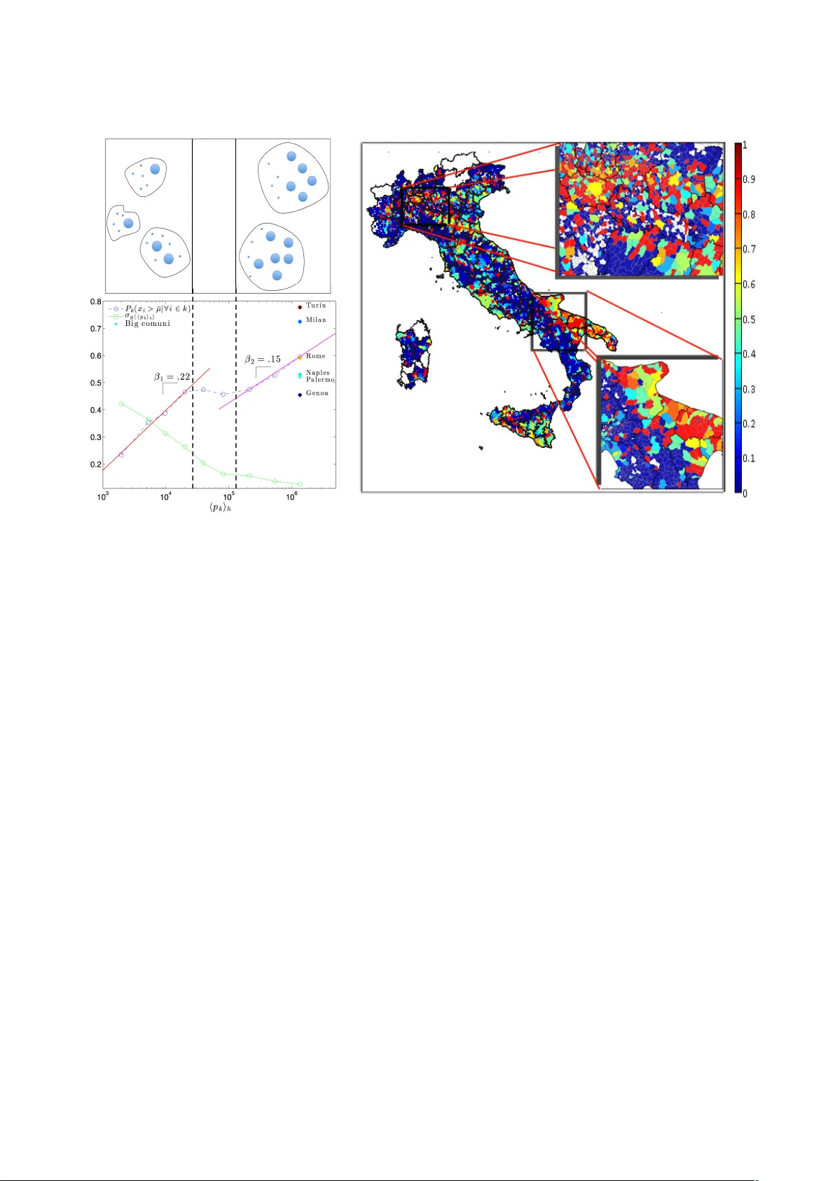
Loading comments...
Leave a Comment