Rapid and deterministic estimation of probability densities using scale-free field theories

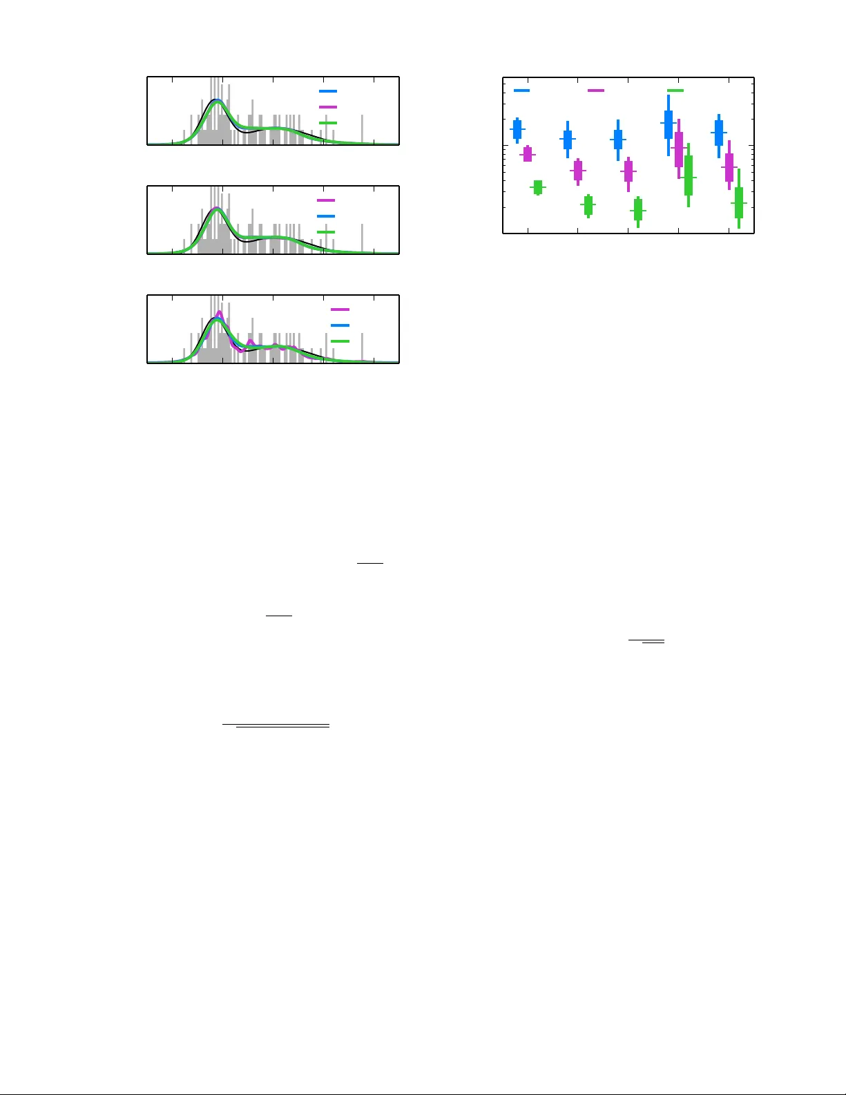
Rapid and deterministic estimation of probabilit y densities using scale-free field theories Justin B. Kinney ∗ Simons Center for Quantitative Biolo gy, Cold Spring Harb or L ab or atory, Cold Spring Harb or, NY, 11724, USA (Dated: 18 April 2014) The question of how b est to estimate a con tinuous probability density from finite data is an in triguing op en problem at the in terface of statistics and physics. Previous w ork has argued that this problem can be addressed in a natural wa y using metho ds from statistical field theory . Here I describ e new results that allo w this field-theoretic approach to be rapidly and deterministically com- puted in low dimensions, making it practical for use in da y-to-day data analysis. Imp ortantly , this approac h does not impose a privileged length scale for smoothness of the inferred probabilit y density , but rather learns a natural length scale from the data due to the tradeoff betw een goo dness-of-fit and an Occam factor. Op en source soft w are implementing this metho d in one and tw o dimensions is pro vided. Supp ose w e are giv en N data p oints, x 1 , x 2 , . . . , x N , eac h of which is a D -dimensional v ector dra wn from a smo oth probabilit y densit y Q true ( x ). How migh t w e esti- mate Q true from these data? This classic statistics prob- lem is known as “density estimation” [1] and is routinely encoun tered in nearly all fields of science. Ideally , one w ould first sp ecify a Bay esian prior p ( Q ) that w eights eac h density Q ( x ) according to some sensible measure of smo othness. One w ould then compute a Bay esian p osterior p ( Q | data) iden tifying which densities are most consisten t with b oth the data and the prior. Ho wev er, a practical implemen tation of this straight-forw ard ap- proac h has yet to be dev elop ed, ev en in low dimensions. This pap er discusses one such strategy , the main the- oretical asp ects of which were w orked out by Bialek et al. in 1996 [2]. One first assumes a sp ecific smo othness length scale ` . A prior p ( Q | ` ) that strongly penalizes fluc- tuations in Q below this length scale is then formulated in terms of a scalar field theory . The maximum a p os- teriori (MAP) density Q ` , whic h maximizes p ( Q | `, data) and serv es as an estimate of Q true , is then computed as the solution to a nonlinear differential equation. This approac h has b een implemented and further elab orated b y others [3–10]; a connection to previous literature on “maxim um p enalized lik eliho o d” [1] should also b e noted. Left lingering is the question of ho w to choose the length scale ` . Bialek et al. argued, how ev er, that the data themselves will t ypically select a natural length scale due to the balancing effects of go o dness-of-fit (i.e. the p osterior probability of Q ` ) and an Occam factor (re- flecting the entrop y of mo del space [11]). Specifically , if one adopts a “scale-free” prior p ( Q ), defined as a lin- ear com bination of scale-dep enden t priors p ( Q | ` ), then the p osterior distribution ov er length scales, p ( ` | data), will b ecome sharply peaked in the large data limit. This imp ortan t insight was confirmed computationally by Ne- menman and Bialek [3] and provides a comp elling alter- nativ e to cross-v alidation, the standard method of select- ing length scales in statistical smoothing problems [1]. Ho wev er computing p ( ` | data) requires first computing Q ` at every relev ant length scale, i.e. solving an infinite comp endium of nonlinear differential equations. Nemen- man and Bialek [3] approac hed this problem b y com- puting Q ` at a finite, pre-selected set of length scales. Although this strategy yielded imp ortant results, it also has significan t limitations. First, it is unclear how to c ho ose the set of length scales needed to estimate Q true to a sp ecified accuracy . Second, as w as noted [3], this strategy is very computationally demanding. Indeed, no implemen tation of this approac h has since b een devel- op ed for general use, and p erformance comparisons to more standard densit y estimation metho ds ha v e y et to b e rep orted. Here I describ e a rapid and deterministic homotopy metho d for computing Q ` to a sp ecified accuracy at all relev ant length scales. This makes low-dimensional den- sit y estimation using scale-free field-theoretic priors prac- tical for use in da y-to-day data analysis. The open source “Densit y Estimation using Field Theory” (DEFT) soft- w are pack age, av ailable at github.com/jbkinney/13_ deft , provides a Python implementation of this algo- rithm for 1D and 2D problems. Simulation tests show fa vorable performance relative to standard Gaussian mix- ture model (GMM) and k ernel densit y estimation (KDE) approac hes [1]. F ollowing [2, 3] we begin by defining p ( Q ) as a linear com bination of scale-dep endent priors p ( Q | ` ): p ( Q ) = Z ∞ 0 d` p ( Q | ` ) p ( ` ) . (1) Adopting the Jeffreys prior p ( ` ) ∼ ` − 1 renders p ( Q ) co- v ariant under a rescaling of x [11]. Our ultimate goal will b e to compute the resulting posterior, p ( Q | data) = Z ∞ 0 d` p ( Q | `, data) p ( ` | data) . (2) As in [3], we limit our attention to a D -dimensional cub e ha ving volume V = L D . W e further assume p erio dic b oundary conditions on Q , and imp ose G D grid p oin ts ( G in each dimension) at which Q will b e computed. 2  4  2 0 2 4 x Q (a)  4  2 0 2 4 x 10  1 10 0 10 1 ` (b) 10  1 10 0 10 1 `  100  80  60  40  20 0 ln p ( ` | data ) (c)  4  2 0 2 4 x Q (d) FIG. 1. (Color) Illustration DEFT in one dimension. (a) An example density Q true ( x ) (black) along with a normal- ized histogram of N = 100 sampled data p oints (gra y). (b) Heat map showing all of the MAP densities Q ` ( x ) computed using α = 2, G = 100, and the data from panel (a); lighter shading corresponds to higher probabilit y . (c) Log posterior probabilit y for eac h length scale ` sho wn in panel (b); the y- axis is shifted so that ln p ( ` ∗ | data) = 0. (d) The MAP densit y Q ∗ ( x ) (blue) along with 20 densities (orange) sampled from p ( Q | data) using Eq. 10. Length scales ` corresp onding to the MAP and sampled densities are shown in panel (c). T o guaran tee that each density is p ositiv e and normal- ized, w e define Q in terms of a real scalar field φ as Q ( x ) = e − φ ( x ) R d D x 0 e − φ ( x 0 ) . (3) Eac h Q corresponds to multiple different φ , but there is a one-to-one corresp ondence with fields φ nc that hav e no constan t F ourier comp onen t. Using this fact, we adopt the standard path integral measure D φ nc as the measure on Q -space, and define the prior p ( Q | ` ) in terms of a field theory on φ nc . In this pap er w e consider the sp ecific class of priors discussed b y [2], i.e. p ( φ nc | ` ) = 1 Z 0 ` exp  − Z d D x ` 2 α − D 2 φ nc ∆ φ nc  . (4) Here w e tak e α to b e a positive integer and define the dif- feren tial operator ∆ = ( −∇ 2 ) α . Z 0 ` is the corresp onding normalization factor. This prior effectively constrains the α -order deriv atives of φ nc , strongly dampening F ourier mo des that ha ve wa velength muc h less than ` . Applying Bay es’s rule to this prior yields the follo wing exact expression for the p osterior [12]: p ( φ nc | `, data) = 1 Z N ` Z ∞ −∞ dφ c e − β S N ` [ φ ] , (5) where S N ` [ φ ] = Z d D x  φ ∆ φ 2 + e t Rφ + e t e − φ V  (6) is the “action” describ ed by [2] and explored in later w ork [3, 8 – 10]. Here, R ( x ) = N − 1 P N n =1 δ ( x − x n ) is the raw data densit y , φ ( x ) = φ nc ( x ) + φ c , t = ln( N /` 2 α − D ), β = ` 2 α − D , and Z N ` = Z 0 ` Γ( N )( V / N ) N p (data | ` ). It should b e noted that [2] used Q ( x ) = const × e − φ ( x ) in place of Eq. 3, and enforced normalization using a delta function factor in the prior p ( Q | ` ); Eq. 6 was then deriv ed using a large N saddle point appro ximation. The alternativ e form ulation in Eqs. 3 and 4 renders the action in Eq. 6 exact. The MAP density Q ` corresp onds to the classical path φ ` , i.e. the field that minimizes S N ` . Setting δ S N ` /δ φ = 0 giv es the nonlinear differen tial equation, ∆ φ ` + e t [ R − Q ` ] = 0 , (7) where Q ` ( x ) = e − φ ` ( x ) /V is the probability densit y cor- resp onding to φ ` . The central finding of this pap er is that, instead of computationally solving Eq. 7 at select length scales ` , w e can compute φ ` at all length scales of interest using a con vex homotopy method [13]. First we differentiate Eq. 7 with resp ect to t , yielding [ e − t ∆ + Q ` ] dφ ` dt = Q ` − R. (8) If we know φ ` at any sp ecific length scale ` i , we can determine φ ` at any other length scale ` f – and at all length scales in b etw een – by integrating Eq. 8 from ` i to ` f . Because S N ` [ φ ] is a strictly conv ex function of φ , eac h φ ` so identified will uniquely minimize this action. Moreo ver, b ecause Eq. 6 is exact, each corresp onding Q ` will fit the data optimally even when N is small. And since the matrix representation of e − t ∆ + Q ` is sparse, dφ ` /dt can b e rapidly computed at each successive v alue of t using standard sparse matrix metho ds. T o iden tify a length scale ` i from whic h to initiate in- tegration of Eq. 8, we lo ok to the large length scale limit, where a w eak-field approximation can be used to compute φ ` i . Linearizing Eq. 7 and solving for φ ` giv es, for | k | > 0, ˆ φ ` ( k ) = − V ˆ R ( k ) 1+exp[ τ k − t ] , where hats denote F ourier trans- forms, k ∈ Z D indexes the F ourier mo des of the v olume V , and eac h τ k = ln[(2 π | k | ) 2 α L D − 2 α ] is a log eigen v alue of V ∆. T o guarantee that none of the F ourier mo des of 3  4  2 0 2 4 x Q (a) ↵ =2 , h =0 . 1 L = 10 L = 30 L = 100  4  2 0 2 4 x Q (b) ↵ =2 , L = 10 h =0 . 3 h =0 . 1 h =0 . 03  4  2 0 2 4 x Q (c) L = 10 , h =0 . 1 ↵ =1 ↵ =2 ↵ =3 FIG. 2. (Color) Robustness of DEFT to changes in runtime parameters. Q ∗ ( x ) was computed using the data from Fig. 1 and v arious choices for (a) the length L of the b ounding b ox, (b) the grid spacing h , and (c) the order α of the deriv ativ e constrained by the field theory prior. L = 10 corresponds to the b ounding box sho wn, and h = 0 . 1 is the grid spacing used for the histogram (gray). Q true ( x ) is shown in black. φ ` i are saturated, ` i should corresp ond to a v alue t i that is sufficien tly less than min | k | > 0 τ k , i.e. ` i  N 1 2 α − D L . Similarly , w e terminate the in tegration of Eq. 8 at a length scale ` f b elo w which Nyquist mo des saturate. This yields the criterion ` f  n 1 2 α − D h where h = L/G is the grid spacing and n = N /G D is the num b er of data p oin ts per v o xel. Ha ving computed φ ` at every relev ant length scale, a semiclassical appro ximation giv es p ( ` | data) = const × e − β S N ` [ φ ` ] p β det[∆ + e t Q ` ] × p ( ` ) . (9) The MAP probability , p ( φ ` | `, data), is represen ted b y the exp onen tial term. This is the “go o dness-of-fit”, which steadily increases as ` gets smaller. This is multiplied b y an Occam factor (the in v erse ro oted quantit y), which steadily decreases as ` get smaller due to the increas- ing entrop y of mo del space. As discussed by [2, 3], this tradeoff causes p ( ` | data) to p eak at a nontrivial, data- determined length scale ` ∗ . The length scale prior p ( ` ) must decay faster than ` − 1 in the infrared in order for p ( ` | data) to be normaliz- able. The need for suc h regularization reflects redun- dancy among the priors p ( φ nc | ` ) for ` > ` i that results from the volume V supp orting only a limited num b er of long wa v elength F ourier mo des. Similar concerns hold in the ultraviolet due to our use of a grid. W e therefore set ↵ =1 ↵ =2 ↵ =3 KDE GMM 10  2 10  1 D ( Q true ,Q ⇤ ) N = 100 N = 1000 N = 10000 FIG. 3. (Color) Comparison of densit y estimation metho ds in one dimension. 10 2 densities Q true ( x ) were generated ran- domly , each as the sum of fiv e Gaussians. Data sets of v arious size N were then drawn from each Q true , after whic h estimates Q ∗ w ere computed using DEFT ( G = 100, v arious α ), KDE (using Scott’s rule to set k ernel bandwidth), and GMM (us- ing the Ba yesian information criterion to choose the num b er of components). Accuracy was quantified using the geo desic distance D geo ( Q true , Q ∗ ) shown in Eq. 11. Box plots indicate the median, interquartile range, and 5%-95% quan tile range of these D geo v alues. p ( ` ) = 0 for ` > ` i and ` < ` f . The p osterior densit y p ( Q | data) can b e sampled by first choosing ` ∼ p ( ` | data), then selecting φ ∼ p ( φ | `, data). This latter step simplifies when p ( ` | data) is strongly p eaked about a sp ecific ` ∗ b ecause, in this case, the eigenv alues and eigenfunctions of ∆ + e t Q ` do not dep end strongly on which ` is selected and therefore need to b e computed only once. p ( φ | `, data) can then b e sampled b y c ho osing φ ( x ) = φ ` ( x ) + G D X j =1 η j p β λ j ψ j ( x ) , (10) where each ψ j is an eigenfunction of the op erator ∆ + e t ∗ Q ∗ satisfying R d D x ψ j ( x ) 2 = 1, λ j is the corresp ond- ing eigen v alue, and eac h η j is a normally distributed ran- dom v ariable. Fig. 1 illustrates k ey steps of the DEFT algorithm. First, the user sp ecifies a data set { x n } N n =1 , a b ounding b o x for the data, and the num b er of grid p oin ts to b e used. A histogram of the data is then computed using bins that are cen tered on eac h grid point (Fig. 1a). Next, length scales ` i and ` f are chosen. Eq. 8 is then inte- grated to yield φ ` at a set of length scales b etw een ` i and ` f c hosen automatically by the ODE solver to ac hiev e the desired accuracy . Eq. 9 is then used to compute p ( ` | data) at each of these length scales, after whic h ` ∗ is identified. Finally , a spec ified num b er of densities are sampled from p ( Q | data) using Eq. 10. DEFT is not completely scale-free b ecause b oth the b o x size L and grid spacing h are pre-specified by the user. In practice, how ev er, Q ∗ app ears to b e v ery insen- sitiv e to the sp ecific v alues of L and h as long as the data 4 Q true N = 30 R ↵ =2 ↵ =3 ↵ =4 KDE GMM N = 300 N = 3000 FIG. 4. Example density estimates in tw o dimensions. Shown is a sim ulated density Q true comp osed of t wo Gaussians, data sets of v arious size N display ed using the raw data density R , and the resulting densit y estimates Q ∗ computed using DEFT ( G = 20), KDE, or GMM as in Fig. 3. The gra yscale in all plots is calibrated to Q true . lie well within the b ounding b ox and the grid spacing is muc h smaller than the inherent features of Q true ; see Figs. 2a and 2b. It is interesting to consider how the choice of α af- fects Q ∗ . As Bialek et al. hav e discussed [2], this field- theoretic approac h pro duces ultra violet divergences in φ ` when α < D / 2. Ab ov e this threshold, increasing α typ- ically increases the smoothness of Q ∗ , although not nec- essarily by muc h (see Fig. 2c). How ever, larger v alues of α may necessitate more data b efore the principal F ourier mo des of Q true app ear in Q ∗ . Increasing α also reduces the sparseness of the ∆ matrix, thereby increasing the computational cost of the homotopy metho d. T o assess how well DEFT p erforms in comparison to more standard density estimation metho ds, a large num- b er of data sets were sim ulated, after which the accu- racy of Q ∗ pro duced by v arious estimators was computed. Sp ecifically , the “closeness” of Q true to each estimate Q ∗ w as quan tified using the natural geo desic distance [14], D g eo ( Q true , Q ∗ ) = 2 cos − 1  Z d D x p Q true Q ∗  . (11) As shown in Fig. 3, DEFT performed substan tially b etter when α = 2 or 3 than when α = 1. This lik ely reflects the smo othness of the sim ulated Q true densities. DEFT out- p erformed the KDE metho d tested here and, for α = 2 or 3, p erformed as well or b etter than GMM. This lat- ter observ ation suggests nearly optimal p erformance by DEFT, since each sim ulated Q true w as indeed a mixture of Gaussians. In tw o dimensions, DEFT shows a remark able abil- it y to discern structure from a limited amoun t of data (Fig. 4). As in 1D, larger v alues of α giv e a smo other Q ∗ . How ev er, DEFT requires substan tially more compu- tational p ow er in 2D than in 1D due to the increase in the num ber of grid p oin ts and the decreased sparsity of the ∆ matrix. F or instance, the computation shown in Fig. 1 to ok ab out 0.3 sec, while the DEFT computations sho wn in Fig. 4 to ok about 1-3 sec eac h [15]. Field-theoretic density estimation faces tw o significant c hallenges in higher dimensions. First, the computational approac h describ ed here is impractical for D & 3 due to the enormous num b er of grid p oints that would b e needed. It should b e noted, how ev er, that the 1D field theory discussed by Holy [4] allows Q ` to b e computed without using a grid. It may b e p ossible to extend this approac h to higher dimensions. The “curse of dimensionalit y” presents a more funda- men tal problem. As discussed by Bialek et al. [2], this manifests in the fact that increasing D requires a pro- p ortional increasing in α , i.e. in one’s notion of “smo oth- ness.” This lik ely indicates a fundamen tal problem with using ∆ = ( −∇ 2 ) α to define high dimensional priors. Using a different op erator for ∆, e.g. one with reduced rotational symmetry , might provide a w ay forw ard. I thank Gurinder A tw al, Anne-Florence Bitb ol, Daniel F errante, Daniel Jones, Bud Mishra, Swagatam Mukhopadh ya y , and Bruce Stillman for helpful conv ersa- tions. Supp ort for this work was provided b y the Simons Cen ter for Quantitativ e Biology at Cold Spring Harb or Lab oratory . ∗ Please direct corresp ondence to jkinney@cshl.edu [1] P . P . B. Eggermont and V. N. LaRiccia, Maximum Pe- nalize d Likeliho o d Estimation: V olume 1: Density Esti- mation (Springer, 2001). [2] W. Bialek, C. G. Callan, and S. P . Strong, Phys. Rev. Lett. 77 , 4693 (1996). [3] I. Nemenman and W. Bialek, Phys. Rev. E 65 , 026137 (2002). [4] T. E. Holy , Phys. Rev. Lett. 79 , 3545 (1997). [5] V. Periw al, Phys. Rev. Lett. 78 , 4671 (1997). [6] T. Aida, Physical review letters 83 , 3554 (1999). [7] D. M. Schmidt, Phys. Rev. E 61 , 1052 (2000). [8] J. C. Lemm, Bayesian Field The ory (Johns Hopkins, 2003). [9] I. Nemenman, Neural Comput. 17 , 2006 (2005). [10] T. A. Enßlin, M. F rommert, and F. S. Kitaura, Phys. Rev. D 80 , 105005 (2009). [11] V. Balasubramanian, Neural Comput. 9 , 349 (1997). [12] The iden tity a − N = 1 Γ( N ) R ∞ −∞ du exp  − N u − ae − u  is used here with a = ( N /V ) R d D x e − φ nc ( x ) and u = φ c . [13] E. L. Allgo wer and K. Georg, Numeric al Continuation Metho ds: A n Intr o duction (Springer, 1990). [14] J. Skilling, AIP Conf. Pro c. 954 , 39 (2007). [15] Computation times were assessed on a computer having a 2.8 GHz dual core pro cessor, 16 GB of RAM, and running the Canop y Python distribution (Enthough t).