Counting Markov Blanket Structures

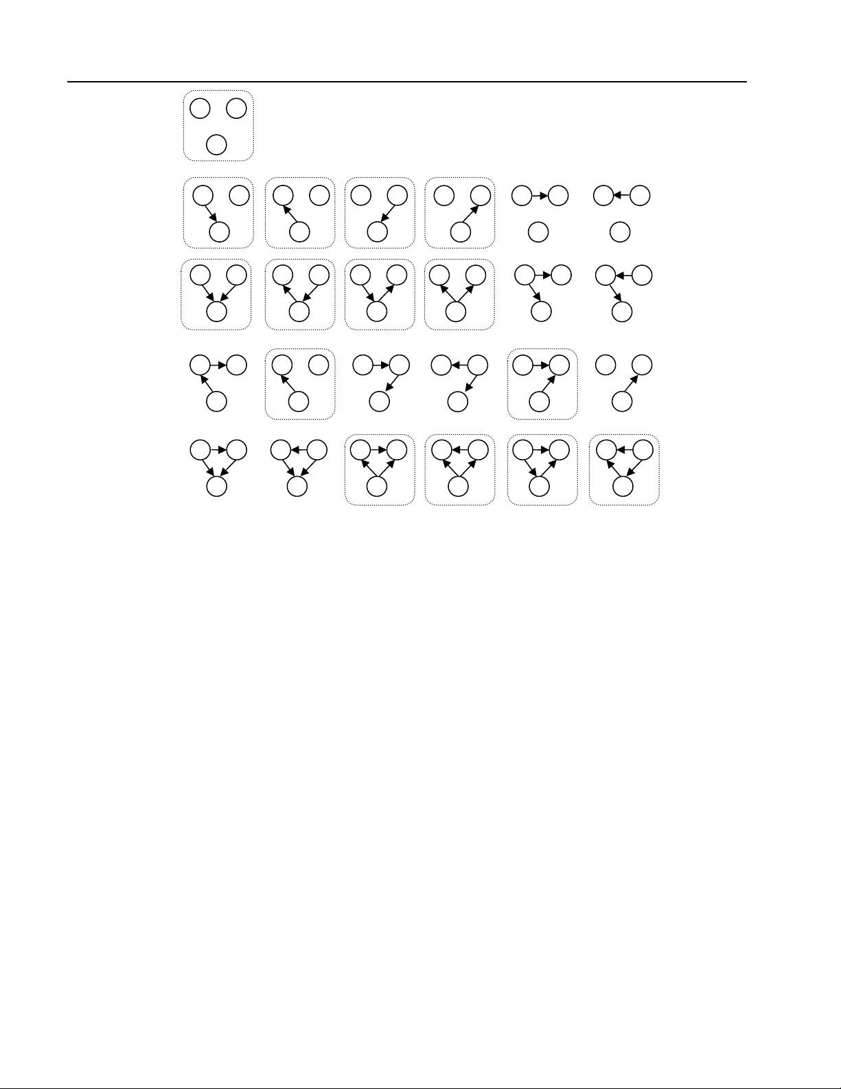
Counting Markov Blanket Struc tur es Shyam Visweswaran, MD, PhD and Gregory F. Cooper, MD, PhD Department of Biomedical Informatics and th e Intelligent Systems Program, University of Pittsburgh School of Medicine, Pittsbu rgh, PA Abstract Learning Markov blanket (MB) structures has proven useful in performing feature selection, learnin g Bayesian networks (BNs), and discovering causal relationships. We present a formul a for efficiently determining the number of MB structures given a target variable and a set of other variables. As expected, the num ber of MB structures grows exponentially. However, we show qu antitatively that there are many fewer MB structures that contain the target variable than there are BN structures that contain it. In particular, the ratio of BN structures to MB structures appears to increase exponential ly in the number of variables. 1. INTRODUCTION An important task i n machine learning an d data mining is to characterize how the target variable is influe nced by other variables in the domain. For example, the goal of a classification or regression algorithm is to learn how the target variable can be best predicted from the other variables. One approach to characterizing the influence on a target variable is to identify a subset of the variables that shields that variable from the influence of other variable s in the domain. Such a subset of variables is called a Markov blanket (MB) of the target variable. As introduced by Pearl (Pearl 1988), the term MB refers to any subset of variables that shield the target variable from the influence of oth er variables in the domain. The minimal Markov blanket or the Markov boundary is a minimal subset of variables that shield the target variable from the influence of other variables in the domain (Pearl 1988). Many authors refer to the minimal Markov b lanket as the Markov blanket, and we follow t his convention. The notion of MB s and the identification of MB s have several uses in machine learning and data mining. The identification of the MB of a variable is useful in the feature (variable) subset selection problem (Koller and Sahami 1996; Ioannis, Constantin et al. 2003). Feature selection is useful in removing irrele vant and redundant variables and in improving the accuracy of classifiers (Dash and Liu 1997) . MB identification can be used for guiding the learning of the graphical structure of a Bayesian network (BN) (Margaritis and Thrun 1999). Identifying MB s is also useful in the discovery of causal structures where the goal is to discover direct causes, direct effects, and common causes of a variable of interest (Mani and Cooper 2004). Several methods of learning BN s f rom data hav e been described in the literature (Cooper and Herskovits 1992; Heckerman, Geiger et al. 1995) . Wh ile the MB of a target variable can be extracted from the BN learned by su ch methods, methods that learn only the MB of a target variable may be more efficient. The general motivati on for searching over the space of MB s is that it is smaller than the space of BN s. Given a set of domain variables, we quantify the size of the MB search space and compare it to the size of the BN search space. W e derive a formula for efficiently determining the number of MB structure s of a target variable given ot her va riables, and we also compute the ratio of BN structures to MB structures for a given number of variables. The remainder of the paper is organized as follows. We review briefly BN s and MB s in Sections 2 and 3. In Section 4, we derive a formula for counting MB s. In Section 5 we compare the number of BN structures and MB structures and in Section 6 we provide a summary of the results. 2. BAYESIAN NETWORKS A Bayesian network is a probabilistic m odel that combines a graphical representation (the BN struct ure) with quantitative information (the BN paramet erization) to represent a joint probability distribution ov er a set of random variables. More specifical ly, a BN representing the set of random variables X i ε X in some domain consists of a pair ( G , Θ G ). The first component G that represents the BN structure is a directed acycl ic graph (DAG) that contains a node for every variable in X and an arc between a pair of nodes if the corresponding variables are directly prob abilistically dependent. Conversely, the absence of an arc between a pair of nodes denotes probabilistic independence between the corresponding variables. Each variable X i is represented by a corresponding node labeled X i in the BN graph, and in the Counting Markov Blanket Structure s this paper we use the terms node and variable interchangeably. The second component Θ G represents the parameterization of the probability distribution over the space of possible instantiations of X and is a set of local probabilist ic models that encode quantitatively the nature of dependence of each node on its parents. For each node X i there is a local probability distribution (that may be discrete or continuous) defined on that node for each state of its parents. The set of all the local pr obability distributions associated with all the nodes comprises a complete parameterizat ion of the BN. Note that the phrase BN structure ref ers only to the graphical structure G , while the term BN (model) refers to both the structure G and a corresponding set of pa rameters Θ G . The terminology of kinship is used to denote various relationships a mong nodes in a BN . These kinship relations are defined along the direction of the arcs. Predecessors of a node X i in G , both immediate and remote, are called the ancestors of X i . In particular, the immediate pr edecessors of X i are called the parents of X i . In a similar fashion, successors of X i in G , both immediate and remote, are called the descendants of X i , and, in particular, the immediate successors are called the children of X i . A node X j is termed a spouse of X i if X j is a parent of a child of X i . The set of nodes consisting of a node X i and its parents is called the family of X i . An example of a BN structure is gi ven in Figure 1(a). A formula for efficiently determining the number of BN structures was first developed by Robinson (Robinson 1971; Robinson 1976), and independently by Stanley (Stanley 1973). The number of BN structures that can be constructed from n variables is given by the following recurrence formula, where BN ( n ) is the number of DAGs that can be constructed give n n nodes:  󰇛  󰇜   󰇛  󰇜    󰇡   󰇢   󰇛  󰇜  󰇛    󰇜      󰇛  󰇜    󰇡   󰇢     󰇛    󰇜  and denotes the number of ways to choose k nodes from n node s. Equation 1 is computed using dynamic programming, namely, the values of BN (*) are computed only once, then cached for whenever they are needed again. The time complexity of computing Equation 1 is O ( n 2 ) where n is the number of variables. From Equation 1, it can be seen that BN ( n ) is com puted from four terms: the first term takes O (1) time, the second term which gives the nu mber of ways to choose k nodes from n nodes takes Figure 1: (a) A BN structure for a do main with 13 variables. The MB of X 7 includes nodes within the circled region, namely, the parents, children and the spouses of X 7 . (b) An example of a MB structure demonstrating various node types. T is the target node, P is a parent node, C is a child node, S is a spousal node, and O is an other node. Note that other nodes are not part of the MB structure and no arcs are allowed between parents or be tween a parent and a spouse (see text). (1) (a) (b) X 1 X 2 X 3 X 4 X 5 X 6 X 7 X 8 X 9 X 10 X 11 X 12 X 13 O O O P P P T S C C O O O Counting Markov Blanket Structure s O ( n 2 ) time, the third term takes O ( n 2 ) time and the fourth term is retrieved in O (1) time from the cache. This analysis assumes that all operations can be done in O (1) time, which is probably a reasonable assumption for n small eno ugh that the operations do not cause an arithmetic ov erflow or underflow. As n gets large, special routines may be needed to handle operations on n , which will increase the time com plexity. 3. MARKOV BLANKETS The MB of a variable X i , denoted by MB ( X i ), defines a set of variables such that conditioned on MB ( X i ), X i is conditionally independent of all variables outside of MB ( X i ). The minimal MB is a minimal set MB ( X i ) conditioned on which X i is conditionally independent of all variables outside of MB ( X i ). As mentioned in the introduction, we shall refer to the minimal MB as the MB. Analogous to BNs, a MB structure refers only to the graphical structure while a MB refers to bo th the structure and a corresponding set of parameters. The MB structure consists of the parents, children, and children’s parents of X i , as illustrated in Figure 1( b) . Different MBs that entail the same factorization for the conditional distribution P ( X i | MB ( X i ) ) belong to the same Markov equivalence class . We define a MB structure specifically as a representative member of a Markov equivalence class that has no arcs between parents or between a parent and a spouse. With respect to a MB structure, the nodes of the BN can be categ orized into five groups: (1) the target node, (2) parent nodes of the target, (3) child nodes of the target, (4) spousal nodes, which are parent nodes of the children, and (5) other nodes, which are not part of the MB. The node under consideration is called the target node. A parent node is one that has an outgoing arc to the target node and may have additional outgoing ar cs to on e or more child nodes. A child node is one that has an incoming arc from the targ et node, m ay have additional incoming arcs from parent nodes, spousal nodes and other child nodes, and may have outgoing arcs to other child nodes. A spousal node is one that has outg oing arcs to one or more child nodes and has neither an incoming arc from the target node nor an outgoing arc to it . An other node is one that is not in the MB and is considered to be a potential spousal node, as we explain below. An example demonstrating the various types of n odes in a MB structure is given in Figure 1(b). As mentioned earlier, i n a MB structure we disallow arcs between parent nodes, arcs between parent no des and s pousal nodes and arcs between child nodes and other nodes. Figure 2: The 2 5 BN structures for a domain containing three variables. The 15 MB structures with respect to variable Z are indicated by dashed boxes around them . X Z Y X Z Y X Z Y X Z Y X Z Y X Z Y X Z Y X Z Y X Z Y X Z Y X Z Y X Z Y X Z Y X Z Y X Z Y X Z Y X Z Y X Z Y X Z Y X Z Y X Z Y X Z Y X Z Y X Z Y X Z Y Counting Markov Blanket Structure s 4. COUNTING MARKOV BLANKET STRUCTURES We now derive of a formula for counting the nu mber of distinct MB structures with respect to a target variable. The number of possible MB structures for a domain with n variables is given by the foll owing equation:  󰇛  󰇜    󰇧 󰇛    󰇜           󰇨                      󰇛   󰇜      󰇛  󰇜               where, n p is number of parent nodes, n c is the number of child nodes, n so is the number of spousal and other nodes, and BN ( n c ) is the number of DAGs that can be constructed with n c nodes and is given by Equat ion 1. Equation 2 is derived as follows. The terms inside the double summation count the number of MB structures for a specified number of n p , n c and n so nodes. The first term gives the number of ways n - 1 can be partitioned into n p parent nodes, n c child nodes and n so sp ousal and other nodes; this term is sometimes called the multiplicity . The second term gives the number of distinct MB structures that differ only in the presence or absence of arcs from parent nodes to child nodes. Each parent node can have an arc to none, one or more child nodes for a total of c n 2 distinct MB structures. For n p parent nodes, the nu mber of distinct MB structures that differ only in the presence or absence of arcs from parent nodes to child nodes is p c n n 2 . The third term gives the number of distinct MB structures that differ only in the presence or absence of arcs from spousal and other nodes to child nodes. This derivation is similar to the derivation of the previous term. Each spousal or other node can have an arc to none, one, or more child nodes for a total of so n 2 distinct MB structures. For n so spousal or other nodes, the number of distinct MB structures that differ only in the presence or absence of arcs from spousal or othe r nodes to child nodes is so c n n 2 . The fourth and last term gives the number of DAGs that can be constructed with n c child nodes. The summation is carried over all possible values of n p and n so ; selection of particular values for n p and n so determines the value of n c and hence no explicit summation is required over the values of n c . Note that the number of parent nodes, the number of child nodes, the number of Table 1: Number of BN structures BN ( n ) and MB structures MB ( n ) as a function of number of nodes n . The number of MB structures is with respect to a single target node and is not a count of all MB structures for all nodes. The last column gives the ratio of the two types of structures. Both BN ( n ) and MB ( n ) are exponential in n . (2) n BN ( n ) MB ( n ) Ratio BN ( n ) / MB ( n ) 1 1 1 1.0 2 3 3 1.0 3 25 15 1.66666666667 4 543 153 3.54901960784 5 29 , 281 3,567 8.20885898514 6 3,781,503 196,833 19.2117327887 7 1,138,779, 265 25 , 604 ,415 44.4758946846 8 783,702, 329 ,343 7,727,833, 473 101.412942202 9 1,213,442, 454 ,842,881 5,321,887, 813 ,887 228.009777222 10 4,175,098, 976 ,430,598, 143 8,241,841, 773 ,665,793 506.573541580 11 31 , 603 ,459, 396 ,418,917, 607 ,425 28 , 359 ,559, 029 ,362,676, 735 1,114.38472522 12 521,939, 651 ,343, 829 ,405, 020 ,504,063 214,672, 167 ,825, 864 ,945, 784 ,833 2,431.33358474 13 1.867660E+031 3.545390E+027 5,267.85556534 14 1.439428E+036 1.268651E+032 11 ,346.1282090 15 2.377253E+041 9.777655E+036 24 ,313.1173477 16 8.375667E+046 1.614805E+042 51 ,867.9742260 17 6.270792E+052 5.689370E+047 110,219.439109 18 9.942120E+058 4.259584E+053 233,405.867102 19 3.327719E+065 6.753420E+059 492,745.716894 20 2.344880E+072 2.260432E+066 1,037,359.40236 21 3.469877E+079 1.592816E+073 2,178,454.74390 22 1.075823E+087 2.356996E+080 4,564,381.36751 Counting Markov Blanket Structure s spousal and other nodes and the single target node together add up to n nodes. Excluding the target node, the sum of the nodes is n – 1. As an example, for a domain containing three variables, the number of BN structures is 25 and the number of MB structures is 15 as given by Equations 1 and 2 respectively. Figure 2 s hows all 25 BN st ructures and indicates the 15 MB structures with resp ect to one of the domain variables. The time complexity of computing Equation 2 is O ( n 2 ) where n is the number of domain variables. From Equation 2, it can be seen that MB ( n ) is computed from four terms: the first term takes O ( n 2 ) time, the second and third terms take O ( n ) time each and the fourth term takes O ( n 2 ) time as derived pre viously for Equation 1. Of note the number of distinct possible MB structures is the same for any variable in a given domain , and thus, Equation 2 applies to an arbitrary domain variable that is considered the target varia ble. 5. A COMPARISON OF THE NUMBER OF BAYESIAN NETWORK AND MARKOV BLANKET STRUCTURES Table 1 gives the values of BN ( n ) and MB ( n ) for n ranging from 0 to 22 where BN ( n ) and MB ( n ) are computed from Equations 1 and 2 respectively . It can be seen from the table that while there are fewer MB structures of the target variable than there are BN structures, the nu mber of MB structures is exponential in the number of variables. Thus, as is generally appreciated, exhaustive search in the space of MB structures will usually be infeasible for domains containing more than a few variables and heuristic search i s appropriate. The last column in Table 1 gives the values of the ratio of BN ( n ) to MB ( n ) for n ranging from 1 to 22. It app ears that this ratio is increasing exponentially in n . Thus, searching in the sp ace of MB structures is likely to be relatively much more efficient than searchi ng in the space of BN structures. 6. SUMMARY We have presented a formula for efficiently determining the number of MB structures without enum erating them explicitly . Although there are fewer MB structures than there are BN structures, the number of MB structures is exponential in the number of variables. However , the ratio of BN structures to MB structures a ppears to i ncrease exponentially in the number of domain variables. Thus, while searching exhaustively in the space of MB structures will usually be infeasible, searching in the space of MB structures is likely to be more efficient than searching in the space of BN structures. Thus, for algorithms that need only learn the MB structure this paper quantifies the degree to which it is preferable to search in the sp ace of MB structures rather than in the space of BN structures. References Cooper, G. F. and E. Herskovits (1992). A Bayesian method for the induction of probabilistic networks from data. Machine Learning 9 (4): 309-347. Dash, M. and H. Liu (1997). Feature selection for classification. Intelligent Data Analysis 1 : 131 – 156. Heckerman, D., D. Geiger, et al. (1995). Learning Bayesian networks - the combination of knowledge and statistical data. Machine Learning 20 (3): 197-243. Ioannis, T., F. A. Constantin, et al. (2003). Time and sample efficient discovery of Markov bla nkets and direct ca usal relat ions. Proceedi ngs of the Ninth ACM SIGKDD International Conference on Knowledge Discovery and Data Min ing, Washington, D.C., ACM. Koller, D. and M. Sahami (1996). Toward optimal feature selection. Proceedings of the Thirteenth International Conference on Machine Learning. Mani, S. and G. F. Cooper (2004). A Bayesian local causal discovery algorithm. Proceedings of the World Congress on Medical Informatics, San Francisco, CA. Margaritis, D. and S. Thrun (1999). Bayesian network induction via local neighborhoods. Proceedings of the 1999 Conference on Advances in Neural Information Processing Systems, Denver, CO, MIT Press. Pearl, J. (1988). Probabilistic Reasoning in Intelligent Systems. San Mateo, California, Morgan Kaufmann. Robinson, R. W. (1971). Counting labeled acyclic digraphs. New Directions in Graph Theory, Third Ann Arbor Conference on Graph Theory, University of Michigan, Academic Press. Robinson, R. W . (1976). Counting unlabeled acyclic digraphs. Proceedings of the Fifth Australian Conference on Combinatorial Mathem atics, Melbourne, Australia. Stanley, R. P. (1973). Acyclic orientations of graphs. Discrete Mathematics 5 : 171- 178.