A Statistical Modelling and Analysis of PHEVs Power Demand in Smart Grids

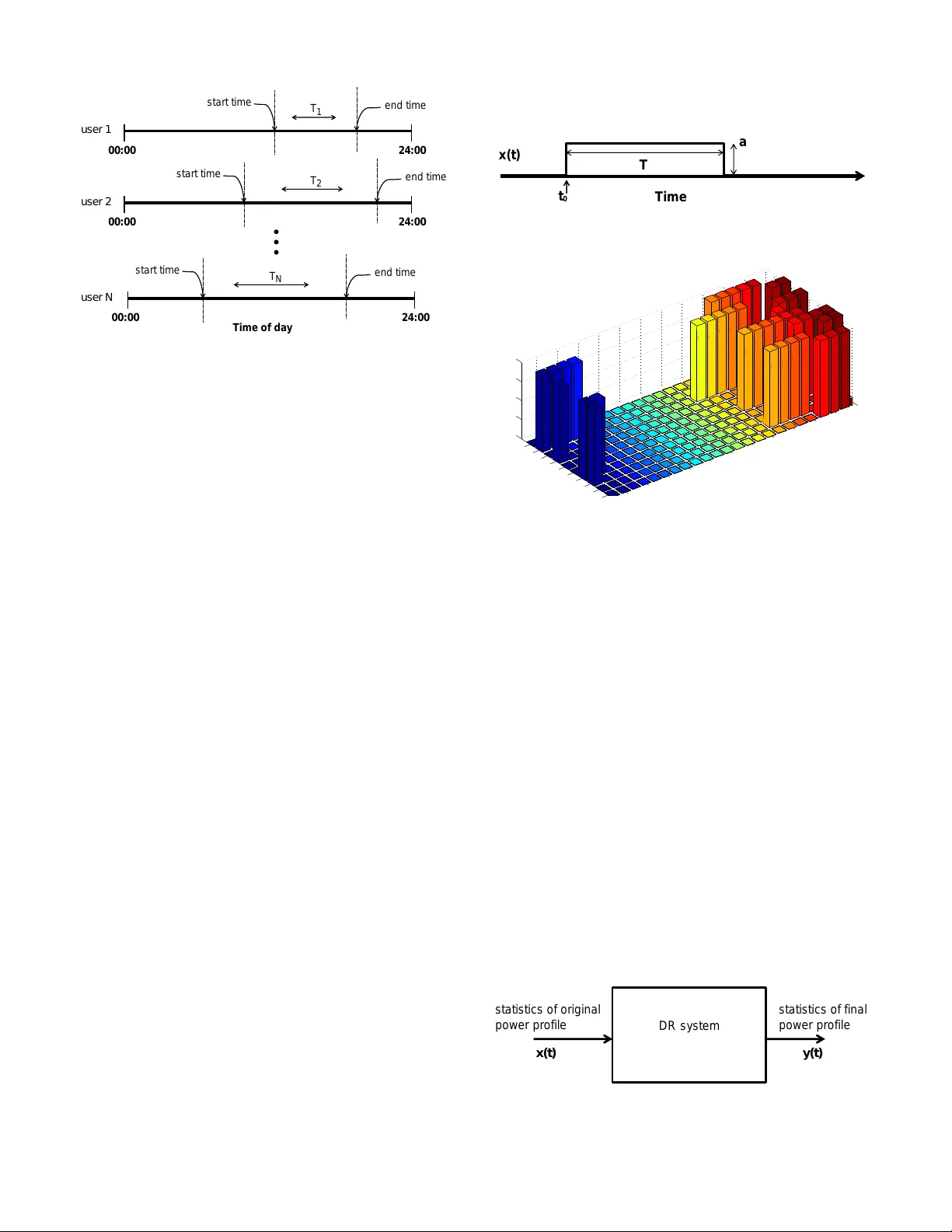
A Statistical Modelling and Analysis of PHEVs’ Po wer Demand in Smart Grids Farshad Rassaei, W ee-Seng Soh and K ee-Chaing Chua Department of Electrical and Computer Engineering National University of Singapore, Singapore Email: { f.rassaei, weeseng, eleckc } @nus.edu.sg Abstract —Electric vehicles (EVs) and particularly plug-in hybrid electric vehicles (PHEVs) are f oreseen to become popular in the near future. Not only are they much mor e en vironmentally friendly than con ventional internal combustion engine (ICE) vehicles, their fuel can also be catered from diverse energy sources and resour ces. However , they add significant load on the power grid as they become widespr ead. The characteristics of this extra load follo w the patterns of people’ s driving behaviours. In particular , random parameters such as arrival time and driven distance of the vehicles determine their expected demand profile from the power grid. In this paper , we first present a model f or uncoordinated charging power demand of PHEVs based on a stochastic process and accordingly we characterize the EV’s expected daily power demand profile. Next, we adopt different distrib utions for the EV’ s charging time follo wing some av ailable empirical resear ch data in the literature. Simulation results show that the EV’s expected daily power demand profiles obtained under the uniform, Gaussian with positive support and Rician distributions for charging time are identical when the first and second order statistics of these distributions are the same. This giv es us useful insights into the long-term planning for upgrading power systems’ infrastructure to accommodate PHEVs. In addition, the results from this modelling can be incorporated into designing demand response (DR) algorithms and evaluating the available DR techniques more accurately . I . I N T R O D U C T I O N The current state-of-the-art in information technology (IT) and data processing are going to be employed extensi vely in smart grids [1]. W idespread deployment of advanced metering infrastructure (AMI) enables real-time and two-way informa- tion exchange between demand side users and the electric utility . This ev olution af fects all different segments of the grid including generation side, transmission, distribution, as well as the demand side. T raditionally , the utility designs and installs the po wer grid’ s infrastructure such that it can provide power to users’ adverse daily power demand profiles similar to that shown in Fig. 1. This po wer demand profile has a significant peak-to-average ratio (P AR) that can potentially reduce the power grids’ efficienc y and incur exorbitant costs for dev eloping the power grid’ s infrastructure, i.e., increasing the po wer generation, transmission, and distribution capacity of the po wer grid. This extra capacity is just to serve the power demand of users during peak-time periods. Therefore, this drawback has motiv ated intensiv e research on strategies that can utilize the existing power grid more efficiently so that more consumers can be accommodated and served without dev eloping new costly 0 2 4 6 8 10 12 14 16 18 20 22 24 0.2 0.25 0.3 0.35 0.4 0.45 0.5 0.55 0.6 0.65 Time of day Demand (kW) Fig. 1. Annual mean daily power demand profile for domestic electricity use in UK [5]. infrastructure. The main objecti ve of these strate gies is to mak e the demand responsive [2]. Similar power efficiency concerns hav e become crucially important for supporting larger number of tenants in green cloud data centres [3]. Demand response (DR) is predicted to become ev en more important as the use of new electricity-hungry appliances such as plug-in electric vehicles (PEVs) or plug-in hybrid electric vehicles (PHEVs) is becoming more widespread. T ypically , on charging mode, they can double the average dwelling’ s energy consumption, with current PHEVs consuming 0.25-0.35 kWh of energy for one mile of driving [4]. On the other hand, PEVs hav e sev eral important advantages compared to internal comb ustion engine (ICE) v ehicles. Not only do they hav e lower maintenance and operation costs, they also produce little or even no air pollution and greenhouse gases in locales where they are being used [6]. Above that, they offer valuable flexibility as their fuel can be catered from div erse sources and resources, e.g., nuclear energy and wind power [7]. Howe ver , in spite of their vast adv antages, the market size of PEVs has been slower than expected as their adoption faces sev eral barriers. One key reason is the extra cost of their batteries. In addition, the shortage of recharging infrastructure causes rang e anxiety for pure electric v ehicles’ dri vers. But, plug-in hybrids resolve the latter problem for pure electric vehicles, by having a combustion engine which works as a backup when the batteries are depleted, yielding to comparable driving ranges for PHEVs to conv entional ICE cars [8]. Although it makes sense to en visage the number of electric cars increasing, it is hard to see that the electricity infrastruc- ture capacity growing with the same rate concurrently . Thus, the ramification of introducing a large number of PHEVs into the grid has become an important avenue for research in recent years [9]. First, we need to ask how uncoordinated charging, i.e., the battery of the vehicle either starts charging as soon as plugged in or after a user-defined delay , can affect the existing power grid. Next, we need to ask, considering this demand as a worst-case scenario, how we can satisfy it efficiently when we hav e information exchange capability and intelligence in a smart grid. There are sev eral prior literature on modelling the impact of uncoordinated charging of PHEVs. Ho wev er, most of them require much detailed information about passenger car travel behaviour , e.g., [10] and [11]. Not only are the models mostly complicated and very test-oriented, but the sensiti vity of the PHEVs’ charging load to different parameters is not also clear . Moreov er , most of them do not provide expected daily power demand due to EVs, particularly when EVs are charged in households rather than in charging stations. For instance, [12] provides a spatial and temporal model of electric vehicles charging demand for fast charging stations situated around highway e xits based on kno wn traf fic data. In [10], a utilization model is proposed based on type-of-trip. The authors in [6] hav e used random simulation and statistical analysis to fit a distribution for the overall charging demand of PHEVs mainly for probabilistic po wer flo w (PPF) calculations. In [13], the daily load profile is modelled by using queuing theory and the approach is suitable mainly for accurate short-time load forecasting. Furthermore, since PHEVs are considered as the main com- ponent of the residential flexible electricity demand, numerous researches hav e been carried out for PHEVs’ DR, e.g., [14] and [15]. Additionally , their storage capacity can be used for improving the power grid’ s reliability , e.g., in terms of frequency control [16]. But, the main drawback in most of these demand response works is that they do not consider the inherent randomness of this demand in the first place. Therefore, in this paper , we present a stochastic model for uncoordinated charging power demand of a typical PHEV by formulating it as a stochastic process based on the arrival time and driv en distance of the vehicles. Moreov er , we deri ve PHEV’ s expected daily power demand according to this model for arbitrary random distributions of arriv al time and charging time. This gives us useful insights into the long-term planning for upgrading the po wer systems’ infrastructure to accommo- date PHEVs. In addition, the results from this modelling can be incorporated into designing DR algorithms and ev aluating the av ailable DR techniques more accurately . The rest of this paper is organized as follows. Section II provides the system model. Statistical analysis is addressed in section III. Numerical results and simulations are represented in section IV. Finally , section V concludes this paper . Energy Source Ret ailer Customer 1 Customer 2 Customer N Energy Market Fig. 2. Basic model of a smart energy system comprised of multiple load customers which share one energy source retailer or an aggregator . Processing agent Flexible load such as PHEV , washing machine, dishwasher , … Inflexible load such as refrigerator , lighting, air conditioning, … User i T o the r etailer Fig. 3. Load segregation of a user according to power demand flexibility . I I . S Y S T E M M O D E L In this section, we describe the energy system model and introduce the layout of this study . Fig. 2 represents a basic power system model where multiple energy customers share one energy source retailer or an aggregator [2] and [17]. Consumers’ total load consists of two different types of load; flexible load and infle xible load (see Fig. 3). Loads which need on-demand power supply (e.g., refrigerators) are considered as inflexible, whereas loads that can tolerate some delays in power supply (e.g., PHEVs) are assumed as flexible loads [17]. Fig. 4 displays the demand flexibility of a flexible appliance for different users. A certain job, ordered by user j , may take time T j to be completed. Moreover , the users set not only the desired job b ut also the deadline by which the job should be accomplished. In this case, we may recognize the following three random variables for a generic flexible appliance: • Start Time shows the time when the user lets the power grid connect to the appliance, and can potentially start deliv ering energy . • Operating Time indicates the time interv al required for accomplishing a certain job, e.g., the ordered charging 00 :00 24 :00 s tart time en d time T use r 2 2 T ime of day 00 :00 24 :00 s tart time en d time T u ser N N 00 :00 24 :00 s tart time e n d t im e T u ser 1 1 Fig. 4. T ime setting for accomplishing a certain job on an appliance for different users during a day . lev els and modes (fast charging or slow charging) for PHEVs, which differs from one user to another . • End Time represents the deadline specified by the user for accomplishing the task of the appliance. Hence, in general, we need to take into account this ran- domness when we in vestigate the overall beha viour of the system. Moreover , to design and analyse DR techniques more accurately , we should consider this stochasticity which comes from the patterns of people’ s li ving behaviours and appliance specifications. Therefore, in general, we can formulate the uncoordinated power consumption for an appliance operating a particular job as follows: x ( t ) , ( a t 0 ≤ t < t 0 + T 0 other wise (1) where we consider instantaneous po wer consumption as a random variable a and assume that power consumption in standby mode is negligible. Additionally , T and t 0 are the operation time and the job’ s start time, respecti vely . These parameters are random in general (see Fig. 5). In addition, here, we are mainly interested in knowing the daily power consumption profiles, i.e., the po wer consumption behaviour throughout a typical 24-hour day . Therefore, we calculate (1) in modulo 24-hours and then project the results onto a 24-hour day . In this case, some realizations of the stochastic process defined in (1) can be displayed as shown in Fig. 6. This figure sho ws (1) for ten dif ferent users in a bar graph with one hour time granularity . Furthermore, a DR technique affects x ( t ) and changes its statistics. This process can be modelled as if x ( t ) is passed through a system as shown in Fig. 7. Therefore, the information about the statistics of the input helps to design the system such that the resulting random process y ( t ) fulfills the desired objectives of the DR techniques. The power consumption profile y ( t ) results from both the DR algorithm T ime T x(t) a t 0 Fig. 5. Demonstration of a typical form of x ( t ) . 2 4 6 8 10 12 14 16 18 20 22 24 1 2 3 4 5 6 7 8 9 10 0 0.5 1 1.5 2 Time Users Demand (kWh) Fig. 6. Some realizations of the stochastic process defined in (1) in modulo 24-hours. and the particular statistics of the original po wer consumption profile. W e can assume probability distribution functions (PDFs) for these two random variables, for instance, according to synthesized models obtained from experimental data, e.g., in [18] for PHEVs. Here, focusing on PHEVs, we assume t 0 and T hav e independent PDFs that can be found from empirical data. For example, for t 0 , as the arriv al time, a Gaussian distribution is suggested in [18]: t 0 ∼ N ( µ, σ 2 ) (2) where µ and σ 2 denote the mean and variance of the Gaussian distribution, respecti vely . For PHEVs, there also exist different charging modes as described in T able I. The charging mode may be considered related to the other random v ariable in (1) which is a . But, we note that there is a tight correlation between a and T . This is obvious due to the fact that on fast charging modes the charging time T is much shorter . statistics of ori gi na l p o w e r p ro file statistics of fina l p o w e r p ro file DR sy stem x(t) y (t) Fig. 7. Demand response technique modelled as a system. T ABLE I D I FFE R E N T T Y PE S OF C H A R G IN G O U T L ET S ( H TT P : / / W W W . T ES L A M OTO R S . CO M / ) OUTLET V/A kW MILES/1-HOUR OF CHARGING Standard 110 / 12 1.4 kW 3 Newer Standard 110 / 15 1.8 kW 4 Single Fast 240 / 40 10 kW 29 T win Fast 240 / 80 20 kW 58 I I I . S TA T I S T I C A L A NA LY S I S In this section, using the aforementioned definition of x ( t ) , we calculate E [ x ( t )] which represents the expected value of power consumption for a certain appliance. This expectation can be expressed by the following proposition for PHEVs (refer to the appendix for the proof). Proposition III.1. Given f t 0 ( · ) and f T ( · ) as the PDFs of the independent random variables arrival time t 0 and char ging time T for a PHEV , the expected uncoordinated char ging power demand can be expr essed as: E [ x ( t )] = a ×  F t 0 ( t ) ∗ [ δ ( t ) − f T ( t )]  (3) in which, ∗ shows the convolution operation and δ ( t ) is the unit impulse function. Also, F ( · ) repr esents the cumulative distribution function (CDF). W e can calculate (3) for any gi ven distribution analytically or numerically . Hereafter , we adopt different distributions for the PHEV’ s charging time T following some av ailable empir- ical research data in the literature, as shown in Fig. 8, to study the corresponding results of (3). W e in vestigate four cases for the distribution of T , namely , the uniform, exponential, Gaussian with positi ve support, and Rician distrib utions. These distributions hav e different degrees of freedom (DoF) and all of them support T over [0 , + ∞ ) : • T : Unif orm In this case, we consider T to hav e uniform distribution over the interv al [ c, d ) . Then, E [ x ( t )] can be analytically deriv ed as stated in the following proposition (see the appendix for the proof). Proposition III.2. Assuming t 0 has a normal distribution with mean µ and variance σ 2 and T has a uniform distrib ution over the interval [ c, d ) , 0 ≤ c < d , the expected uncoor dinated char ging power demand becomes: E [ x ( t )] = a ×  1 − Q ( t − µ σ ) + σ d − c ( c 0 Q ( c 0 ) − d 0 Q ( d 0 ) + f ( d 0 ) − f ( c 0 ) + d 0 − c 0 )  (4) wher e c 0 = t − c − µ σ , d 0 = t − d − µ σ . Also, Q ( x ) and f ( x ) ar e defined as follows: 0 2 4 6 8 10 12 14 16 18 20 0 0.02 0.04 0.06 0.08 0.1 0.12 0.14 0.16 0.18 0.2 T Probability Uniform Exponential Gaussian with positive support Rician Fig. 8. Uniform, exponential, Gaussian with positive support and Rician distributions for T . Q ( x ) = 1 √ 2 π ∞ Z x exp( − u 2 2 ) du, f ( x ) = exp( − x 2 2 ) √ 2 π . • T : Exponential The driven distance and hence the charg- ing time of an EV can be modelled by an exponential distribution [19]. For an exponentially distributed T with mean λ − 1 , we hav e the following PDF: f T ( T ) = λ exp( − λT ) . (5) • T : Gaussian When T has a Gaussian PDF with positiv e support as sho wn in Fig. 8, T has the following distribu- tion function: f T ( T ) = N ( T ; µ, σ 2 | 0 ≤ T < ∞ ) , (6) = 1 Q ( − µ σ ) √ 2 π σ 2 exp( − ( T − µ ) 2 2 σ 2 ) , 0 ≤ T < ∞ . (7) • T : Rician Finally , we consider a Rician PDF for T having the following form: f ( T | ν, σ ) = T σ 2 exp( − ( T 2 + σ 2 ) 2 σ 2 ) I 0 ( T ν σ 2 ) (8) where ν ≥ 0 and σ ≥ 0 present the noncentrality parameter and scale parameter , respecti vely . I 0 ( · ) is the modified Bessel function of the first kind with order zero. I V . S I M U L A T I O N R E S U LT S In this section, we consider Gaussian distribution for the random variable t 0 as the arriv al time with µ = 19 and σ 2 = 10 inspired from [18]. Furthermore, we consider four cases for the distribution of the random variable T as described in section III. First, we consider T to have a uniform 0 2 4 6 8 10 12 14 16 18 20 22 24 0 0.2 0.4 0.6 0.8 1 1.2 1.4 Time Demand (kW) Uniform Exponential Gaussian with Positive Support Rician Fig. 9. A PHEV’ s expected daily power demand profile for different distributions of charging time T . distribution ov er the interval [1 , 11] . Thus, it will hav e µ = 6 and σ 2 = 8 . 33 . Second, we assume T to be exponentially distributed with mean µ = 6 . Third, we assume T to be Gaussian distributed with positiv e support as presented in (7). In this case, we use the well-known accept-reject approach to generate the random values. Finally , we consider a Rician distribution for T . In all cases (except for the exponential distribution), we set the parameters of the distributions such that they all have the same mean and variance. Howe ver , for the exponential distrib ution case, we can only set either its mean or variance to be the same as that of the others since this distribution has just one DoF . Based on an av erage 0.25 kWh energy consumption for each mile of driving, we set all the parameters in (1). In addition, we assume a system comprising of N = 100 , 000 PHEV users in our simulations in order to obtain smooth curves representing the probabilistic expectation. The results for the e xpected daily po wer demand of a typical PHEV under the aforementioned settings are illustrated in Fig. 9. As can be observed, the expected daily power demand resulting from the charging time distributions which possess the same mean and variance tends to the same power profile. Howe ver , for the exponential distribution, since it has only one DoF , we see that its expected power demand differs significantly from that of the others. Based on our proposed model and the obtained results, we observe that the expected uncoordinated charging power demand for a typical PHEV is much lar ger during 6 p.m. to 1 a.m. compared to that during 8 a.m. to 2 p.m. in a one-day frame. Next, in Fig. 10, we compare our obtained analytical result for the expected power demand according to a uniform distri- bution of T in proposition (III.2) with the simulation results in a one-day frame. As can be seen in this figure, the simulation results follo w proposition (III.2) closely , af firming the acquired formulation. 0 2 4 6 8 10 12 14 16 18 20 22 24 0 0.2 0.4 0.6 0.8 1 1.2 1.4 Time Demand (kW) Analytical Simulation Fig. 10. A PHEV’ s expected daily power demand profile for a uniform distribution of charging time T . V . C O N C L U S I O N A N D F U T U R E W O R K In this paper, we discussed the inherent randomness in the demand for flexible appliances in general and for PHEVs in particular . W e considered random distributions for the arriv al time and the charging time of PHEVs inspired by av ailable empirical data in the literature. Accordingly , we presented the uncoordinated charging power demand impact of a PHEV as a stochastic process based on these random v ariables. Next, we derived the expected daily power consumption profile according to this random process. Our simulation results show that the EV’ s expected daily power demand profiles obtained under the uniform, Gaussian with positi ve support and Rician distributions for charging time are identical when the first and second order statistics of these distributions are the same. Our obtained results introduce a simple description for the e xpected power demand of a typical PHEV and hence gi ve us insights into the effect of adding each PHEV into the power system. The study presented in this paper can be extended and de- veloped in various ways. For example, the conv ergence of the daily po wer demand for the aforementioned distributions needs to be prov en. In addition, the results from this modelling can be incorporated into designing DR algorithms and ev aluating the av ailable DR techniques more accurately . A P P E N D I X A. Pr oof of pr oposition III.1: Since x ( t ) = 0 for t 0 ≤ t − T and t ≤ t 0 . Then, E [ x ( t )] becomes: E [ x ( t )] = a × P ( t 0 ≤ t ≤ t 0 + T ) = a × P ( t − T ≤ t 0 ≤ t ) . (9) Further , we can use the total probability theor em [20] to get E [ x ( t )] = a × ∞ Z 0 P ( t − T ≤ t 0 ≤ t | T = T 0 ) f T ( T 0 ) dT 0 = a × ∞ Z 0 ( F t 0 ( t ) − F t 0 ( t − T 0 )) f T ( T 0 ) dT 0 (10) = a ×   F t 0 ( t ) − ∞ Z 0 F t 0 ( t − T 0 ) f T ( T 0 ) dT 0   (11) for which we hav e taken into account the facts that ∞ R 0 f T ( T 0 ) dT 0 = 1 , and t 0 and T are independent. Fur- thermore, we can express (11) in a more concise form by using the definition of the con volution integral and the identity f ( t ) ∗ δ ( t ) = f ( t ) as follo ws: E [ x ( t )] = a × ( F t 0 ( t ) ∗ [ δ ( t ) − f T ( t )]) . (12) B. Pr oof of pr oposition III.2: Since T is uniformly distributed over the interval [ c, d ) , 0 ≤ c < d , we can write (11) as follows: E [ x ( t )] = a ×   F t 0 ( t ) − 1 d − c d Z c F t 0 ( t − T 0 ) dT 0   . (13) Then, by changing the integration v ariable from T 0 to α = t − T 0 , it can be rewritten as follows: E [ x ( t )] = a ×   F t 0 ( t ) + 1 d − c t − d Z t − c F t 0 ( α ) dα   . (14) Further , we need to replace α with β = α − µ σ to have E [ x ( t )] = a ×    F t 0 ( t ) + σ d − c t − d − µ σ Z t − c − µ σ F t 0 ( β ) dβ    (15) in order to be able to use the following formula for a standard normal random v ariable with CDF F ( · ) and PDF f ( · ) to calculate the last term in (15): Z F ( x ) dx = xF ( x ) + f ( x ) + c. (16) Also, we now set c 0 = t − c − µ σ and d 0 = t − d − µ σ for simplicity to express (15) in the following form: E [ x ( t )] = a ×  1 − Q ( t − µ σ ) + σ d − c ( c 0 Q ( c 0 ) − d 0 Q ( d 0 ) + f ( d 0 ) − f ( c 0 ) + d 0 − c 0 )  (17) in which we used the equation F ( x ) = 1 − Q ( x ) . R E F E R E N C E S [1] A. Ipakchi and F . Albuyeh, “Grid of the future, ” P ower and Energy Magazine, IEEE , vol. 7, no. 2, pp. 52 –62, Apr . 2009. [2] A. Mohsenian-Rad, V . W ong, J. Jatskevich, R. Schober , and A. Leon- Garcia, “ Autonomous demand-side management based on game- theoretic ener gy consumption scheduling for the future smart grid, ” IEEE T ransactions on Smart Grid , vol. 1, no. 3, pp. 320 –331, Dec. 2010. [3] A. Dalvandi, M. Gurusamy , and K. C. Chua, “Time-a ware vm-placement and routing with bandwidth guarantees in green cloud data centers, ” in Cloud Computing T echnology and Science (CloudCom), 2013 IEEE 5th International Conference on , vol. 1, Dec 2013, pp. 212–217. [4] J. V an Roy , N. Leemput, F . Geth, R. Salenbien, J. Buscher , and J. Driesen, “ Apartment building electricity system impact of operational electric vehicle charging strategies, ” IEEE T ransactions on Sustainable Ener gy , vol. 5, no. 1, pp. 264–272, Jan. 2014. [5] I. Richardson, M. Thomson, D. Infield, and C. Clifford, “Domestic electricity use: A high-resolution energy demand model, ” Ener gy and Buildings , vol. 42, no. 10, pp. 1878–1887, 2010. [6] G. Li and X.-P . Zhang, “Modeling of plug-in hybrid electric vehicle charging demand in probabilistic power flow calculations, ” IEEE T rans- actions on Smart Grid , vol. 3, no. 1, pp. 492–499, Mar . 2012. [7] W . Shireen and S. Patel, “Plug-in hybrid electric vehicles in the smart grid environment, ” in T ransmission and Distribution Conference and Exposition, 2010 IEEE PES , Apr . 2010, pp. 1–4. [8] D. Callaway and I. Hiskens, “ Achie ving controllability of electric loads, ” Pr oceedings of the IEEE , vol. 99, no. 1, pp. 184–199, 2011. [9] S. Shao, M. Pipattanasomporn, and S. Rahman, “Challenges of PHEV penetration to the residential distribution network, ” in IEEE P ower Ener gy Society General Meeting, 2009. PES ’09 , Jul. 2009, pp. 1–8. [10] P . Grahn, K. Alvehag, and L. Soder , “PHEV utilization model consider- ing type-of-trip and recharging flexibility , ” IEEE T ransactions on Smart Grid , vol. 5, no. 1, pp. 139–148, Jan. 2014. [11] T . K. Lee, B. Adornato, and Z. Filipi, “Synthesis of real-world driving cycles and their use for estimating PHEV energy consumption and char g- ing opportunities: Case study for Midwest/U.S.” IEEE T ransactions on V ehicular T echnology , vol. 60, no. 9, pp. 4153–4163, Nov . 2011. [12] S. Bae and A. Kwasinski, “Spatial and temporal model of electric v ehicle charging demand, ” IEEE T ransactions on Smart Grid , vol. 3, no. 1, pp. 394–403, Mar . 2012. [13] M. Alizadeh, A. Scaglione, J. Davies, and K. Kurani, “ A scalable stochastic model for the electricity demand of electric and plug-in hybrid vehicles, ” IEEE T ransactions on Smart Grid , vol. 5, no. 2, pp. 848–860, Mar . 2014. [14] K. Clement-Nyns, E. Haesen, and J. Driesen, “Coordinated charging of multiple plug-in hybrid electric vehicles in residential distribution grids, ” in P ower Systems Conference and Exposition, 2009. PSCE ’09. IEEE/PES , Mar . 2009, pp. 1–7. [15] ——, “The impact of charging plug-in hybrid electric vehicles on a residential distribution grid, ” IEEE Tr ansactions on P ower Systems , vol. 25, no. 1, pp. 371–380, Feb 2010. [16] M. R. V . Moghadam, R. Zhang, and R. T . Ma, “Randomized response electric vehicles for distributed frequency control in smart grid, ” in 2013 IEEE International Conference on Smart Grid Communications (SmartGridComm) , Oct. 2013, pp. 139–144. [17] A. Mohsenian-Rad and A. Leon-Garcia, “Optimal residential load con- trol with price prediction in real-time electricity pricing environments, ” IEEE T ransactions on Smart Grid , vol. 1, no. 2, pp. 120 –133, Sep. 2010. [18] T . K. Lee, Z. Bareket, T . Gordon, and Z. Filipi, “Stochastic modeling for studies of real-world PHEV usage: Driving schedule and daily temporal distributions, ” IEEE T ransactions on V ehicular T echnology , vol. 61, no. 4, pp. 1493–1502, May 2012. [19] H. Liang, A. T amang, W . Zhuang, and X. Shen, “Stochastic information management in smart grid, ” IEEE Communications Surveys T utorials , vol. Early Access Online, 2014. [20] H. Kobayashi, B. L. Mark, and W . T urin, Pr obability , Random Pro- cesses, and Statistical Analysis: Applications to Communications, Signal Pr ocessing, Queueing Theory and Mathematical Finance . Cambridge Univ ersity Press, 2012.