Discussion of "Single and Two-Stage Cross-Sectional and Time Series Benchmarking Procedures for SAE"

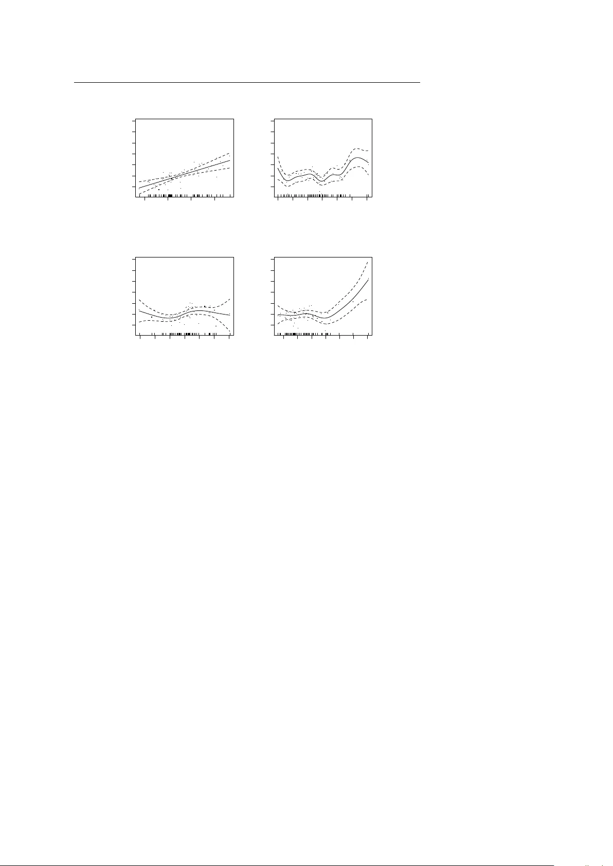
TEST man uscript No. (will b e inserted b y the editor) Discussion of Single and Two-Stage Cr oss-Se ctional and Time Series Benchmarking Pr o c e dur es for SAE Reb ecca C. Steorts · M. Dolores Ugarte Received: date / Accepted: date W e congratulate the authors for a stim ulating and v aluable manuscript, pro- viding a careful review of the state-of the-art in cross-sectional and time-series b enc hmarking procedures for small area estimation. They dev elop a no v el t wo- stage benchmarking method for hierarc hical time series models, where they ev aluate their pro cedure by estimating monthly total unemplo yme n t using data from the U.S. Census Bureau. W e discuss three topics: linearit y and mo del missp ecification, computational complexity and mo del comparisons, and, some asp ects on small area estimation in practice. More specifically , w e p ose the fol- lo wing questions to the authors, that they may wish to answer: How robust is their mo del to missp ecification? Is it time to p erhaps mov e aw a y from linear mo dels of the type considered by ( Battese et al. 1988 ; F a y and Herriot 1979 )? What is the asymptotic computational complexity and what comparisons can b e made to other mo dels? Should the b enchmarking constraints b e inherently fixed or should they b e random? 1 Linearity and Model Missp ecification The authors review previous work in cross-sectional and time-series b ench- marking thoroughly , and prop ose a new cross-sectional tw o-stage time series b enc hmarking metho d. This method is mathematically well-posed and care- fully thought-through. It is applied to the estimation of unemploymen t totals Rebecca C. Steorts Department of Statistics, Carnegie Mellon Universit y Baker Hall 132, Pittsburgh, P A 15213 E-mail: bek a@cmu.edu M. Dolores Ugarte Department of Statistics and O.R., Public Univ ersity of Nav arre Campus de Arrosadia, 31006 Pamplona E-mail: lola@unav arra.es 2 Discussion of Pfeffermann et al. ( 2014 ) at the state-lev el and census-divisions (aggregate state-level estimates). How- ev er, w ith resp ect to mo del v alidity , the analysis do es not go b eyond ev aluat- ing co efficients of v ariation with resp ect to the direct estimates. F urthermore, although the application here may satisfy the mo deling assumptions, it is im- p ortan t that metho ds are built to b e robust to general mo del missp ecification. As one of the authors recently writes, c hec king model v alidity is v ery imp or- tan t in small area estimation ( Pfeffermann 2013 ). The metho d prop osed here relies on a form of the celebrated F a y-Herriot mo del ( F a y and Herriot 1979 ). That mo del, and that of Battese et al. ( 1988 ), w ere ma jor achiev ements for small area estimation, but rest on simplifying assumptions, especially of linearity , whic h are not alwa ys v alid. These mo deling assumptions w ere not chec k ed in Pfeffermann et al. ( 2014 ), and we are unable to c hec k them ourselv es since the cov ariates are not given. 1 T o illustrate what w ould b e inv olved in such a c heck, ho w ev er, we lo ok at cross-sectional data on c hild p ov ert y from the the Small Area and Income Po v erty Estimate (SAIPE) Program at the U.S. Census Bureau. 2 The resp onse v ariable is the rate of c hild p ov erty in eac h state (in 1998), and the cov ariates are an IRS income- tax-based pseudo-estimate of the c hild p o v erty rate, the IRS non-filer rate, the rate of foo d stamp usage, and the residual term from the regression of the 1990 Census estimated child p ov erty rate. W e fit an additive mo del, which strictly nests the linear model implied by the F a y-Herriot assumptions. Figure 1 sho ws the estimated partial resp onse functions, which are clearly nonlinear for three of the four co v ariates. If, on examination, the data in Pfeffermann et al. ( 2014 ) are not linear, then the exact metho d they prop ose do es not apply . How ev er, semiparametric and non-linear mo dels are also av ailable in the small area literature. F or exam- ple, mo dels including p enalized splines (P-splines) hav e b een already used. In particular, Ugarte et al. ( 2009 ) use P-splines to model and forecast dwelling prices in the different neighbourho o ds of a Spanish cit y and Militino et al. ( 2012 ) use P-splines to estimate the p ercentage of fo o d exp enditure for alter- nativ e household sizes at pro vincial level in Spain using the Spanish Household Budget Surv ey . Generalized linear mixed mo dels are also common in disease mapping, an imp ortan t application of small area estimation. F or details, see Ugarte et al. ( 2014 ) and references therein. It seems important to determine ho w robust the Pfeffermann et al. ( 2014 ) method is to nonlinearit y , and ho w it m ust b e mo dified to handle highly nonlinear systems. 1 It w ould b e easier to p erform such chec ks, and to make comparisons to our metho ds, if the co de and data were made publicly av ailable. This has b een done for small area mo dels by Molina and Marhuenda ( 2013 ), and advocated for statistical computation more generally by Sto dden et al. ( 2013 ). 2 This dataset was used before in Datta et al. ( 2011 ), with a F ay-Herriot model, and is publicly av ailable at http://www.census.gov/did/www/saipe/data/statecounty/data/ 1998.html . Discussion of Pfeffermann et al. (2014) 3 10 15 20 25 -5 0 5 10 15 20 25 IRS child poverty rate estimate Partial response 6 8 10 12 14 16 18 -5 0 5 10 15 20 25 IRS non-filer rate Partial response -3 -2 -1 0 1 2 3 -5 0 5 10 15 20 25 1990 Census residuals Partial response 4 6 8 10 12 14 16 -5 0 5 10 15 20 25 Food-stamp rate Partial response Fig. 1 Fitting of a generalized additive mo del to the 1998 SAIPE data. The top left plot is fairly linear, whereas the others deviate from linearity , suggesting the need for either a transformation or a nonparametric approach. In any case, this suggests that as in other dis- ciplines non-linear models (e.g., generalized linear mixed mo dels, kernel smo others, splines) may b e go o d directions to explore. 2 Time Complexity , Model Comparisons, and Benchmarking Benc hmarking requires that estimates at a lo w er level of aggregation (p erhaps coun ties) must match the estimates at a lev el of higher aggregation (the state total for example). Pfeffermann ( 2013 ) and Pfeffermann et al. ( 2014 ) discussed man y adv ances in small area estimation and b enchmarking, making the nov el con tributions very clear in terms of metho dological adv ancements. 2.1 Time complexit y and Mo del Comparisons The procedure of Pfeffermann et al. ( 2014 ) is not the first attempt at t wo- stage b enchmarking for time series. The k ey difference b etw een their metho d, and the earlier one of Ghosh and Steorts ( 2013 ), is that the newer pro cedure cannot be calculated at once, but must be computed in tw o separate stages. It is not clear to us ho w one ought to choose b etw een these metho ds in an y 4 Discussion of Pfeffermann et al. ( 2014 ) particular application. A sensible reason to prefer one method w ould be that its underlying model fits b etter. This raises issues of model specification, as w e mentioned ab ov e, as well as mo del c omp arison . The latter is not discussed b y Pfeffermann et al. ( 2014 ), but would seem to deserve serious attention. Another, less statistical criterion for c ho osing betw een metho ds w ould com- putational complexit y , how ever it is not clear which will always b e the clear winner. The Bay esian approach of Ghosh and Steorts ( 2013 ) must w ait for the Mark ov chain Monte Carlo to come close to con v ergence, but once it has a p osterior sample, estimation is instan taneous, since most solutions are Bay es estimators in a reduced action space. F or Pfeffermann et al. ( 2014 ), on the other hand, we ask what is the computational complexit y of their metho d (and empirically ho w fast is it)? This requires further analysis. 2.2 Benc hmarking with Error Pfeffermann et al. ( 2014 ) clearly explain the distinction b etw een external and internal b enchmarking. W e fo cus here on external b enchmarking, where there is an additional source of information that can b e used for the purp ose of the b enc hmarking pro cedures. Many pap ers hav e included external b enc hmarking in the last few y ears. F or example, se e Datta et al. ( 2011 ), Ghosh and Steorts ( 2013 ) and Bell et al. ( 2013 ) for details. Pro duction of small area estimation motiv ates “traditional” Ba yesian b ench- marking, wherein sub-domain estimates are optimized sub ject to the constraint that the weigh ted av erage equals some total for the domain (usually the direct estimate) ( Datta et al. 2011 ; Ghosh and Steorts 2013 ; Pfeffermann et al. 2014 ; W ang et al. 2008 ). This is effective when, for example, the goal is to matc h a di- rect domain estimate. Ho w ev er, it do es not address situations where the direct estimate is imprecise, there is additional information at the domain level (e.g., an indirect estimate), or the domain is itself a sub-domain of a higher level. In suc h situations, it is more natural to treat the additional information as ran- dom rather than fixed. Thus, instead of making it a hard external constraint, it should b e embedded into a probabilistic mo del, along with the sub-domain data. W e bring this up because it is hard to believe that the direct domain estimates used in Pfeffermann et al. ( 2014 ) are fixed and without error. The uncertain ty in these “external” quantities ought to b e incorp orated into the b enc hmarking, using the kind of probabilistic approach just mentioned. Pre- liminary inv estigations ( Steorts and Louis 2014 ) suggest that under normality and linearity , suc h em b eddings may pro duce almost the same results as the “traditional” approach. This equiv alence breaks down as we mov e aw ay from normalit y and linearity . Ev en if the specific application of Pfeffermann et al. ( 2014 ) does pro v e to b e nearly-linear and nearly-Gaussian, non-linearit y and non-normalit y are important in modern applications. W e w ould v ery m uc h lik e Discussion of Pfeffermann et al. (2014) 5 to see Pfeffermann et al. ( 2014 ) tak e up the challenge of probabilistic external b enc hmarking. 3 Small Area in Practice Man y users of small area estimation are more interested in practical consider- ations than in the underlying theory . Given the metho ds of Pfeffermann et al. ( 2014 ) for tw o-stage b enchmarking and those of Ghosh and Steorts ( 2013 ), the adv antages and disadv antages of each approac h are not clear except in the ob vious case when the benchmarking needs to be separated in to a tw o-step pro cedure due to a time-series as Pfeffermann et al. ( 2014 ) describ es. It would p erhaps b e helpful if the authors could provide some practical guidance as to the b enefits of their prop osed metho dology , as well as examples of settings in whic h they may outp erform other approaches in the literature. In the simulation study , the authors considered a reasonable num ber of small areas and time p oints. How ev er, this might not b e the case in many practical situations and typically out of sample areas could be presen t as the domains b ecome increasing smal l . Examples include certain regions, pro vinces, and de- partmen ts of Europ e. In the United States, geographical regions include states, coun ties, regions, blo cks, blo ck-groups, etc. Can the same type of conclusions b e made if the n um ber areas and time p oints are b oth smaller (and in the presence of out of sample areas)? In addition, the authors giv e an applica- tion, dealing with states and census divisions, where the census divisions are aggregations of the states. Ho w man y of the states and census divisions are small areas after 2000 in terms of the coefficient of v ariation? Clarification here w ould be helpful tow ards practical applications to muc h smaller regions that are of in terest. T o summarize, do the methods alw a ys hold in practice and if not, when do they break do wn? W e again emphasize the contributions from the authors hav e made regarding b oth a review of b enchmarking and a no vel extension to b enchmarking in time series. These hav e led us to ask important questions surrounding mo del missp ecification, linearit y , external b enchmarking, and computational costs. Are we approaching b enchmarking and small area metho ds in the most sound w ay , and if not, what should change? A cknow le dgements Research b y R. Steorts w as supp orted b y the National Sci- ence F oundation through gran ts SES1130706 and DMS1043903 and research b y M. Dolores Ugarte was supp orted by the Spanish Ministry of Science and Inno v ation (pro ject MTM2011-22664 which is co-funded b y FEDER grants). 6 Discussion of Pfeffermann et al. ( 2014 ) References Ba ttese, G. , Har ter, R. and Fuller, W. (1988). An error-comp onents mo del for prediction of count y crop area using survey and satellite data. Journal of the Americ an Statistic al Asso ciation , 83 28–36. Bell, W. , Da tt a, G. and Ghosh, M. (2013). Benc hmarked small area estimators. Biometrika , 100 189–202. D a tt a, G. , Ghosh, M. , Steor ts, R. and Maples, J. (2011). Bay esian b enc hmarking with applications to small area estimation. T est , 20 574–588. F a y, R. and Herriot, R. (1979). Estimates of income from small places: an application of James-Stein pro cedures to census data. Journal of the A meric an Stastic al Asso ciation , 74 269–277. Ghosh, M. and Steor ts, R. (2013). Two-stage bay esian benchmarking as applied to small area estimation. TEST , 22 670–687. Militino, A. F. , Goico a, T. and Ugar te, M. D. (2012). Estimating the p ercen tage of foo d expenditure in small areas using bias-corrected p-spline based estimators. Computational Statistics and Data Analysis , 53 3616– 3629. Molina, I. and Marhuenda, Y. (2013). P ack age sae. URL http://cran. r- project.org/web/packages/sae/sae.pdf . Pfeffermann, D. (2013). New imp ortant dev elopments in small area esti- mation. Statistic al Scienc e , 28 40–68. Pfeffermann, D. , Siko v, A. and Tiller, R. (2014). Single and tw o-stage cross-sectional and time series benchmarking procedures for small area es- timation. TEST . Steor ts, R. and Louis, T. (2014). Constrained bay esian b enchmarking. In Pr ep ar ation . Stodden, V. , Bor wein, J. and Bailey, D. H. (2013). Setting the default to repro ducible in computational science researc h. SIAM News, June , 3 . Ugar te, M. D. , Adin, A. , Goicoa, T. and Militino, A. F. (2014). On fitting spatio-temp oral disease mapping mo dels using approximate ba yesian inference. Statistic al Metho ds in Me dic al R ese ar ch DOI: 10.1177/0962280214527528. Ugar te, M. D. , Goico a, T. , Militino, A. F. and Durb ´ an, M. (2009). Spline smo othing in small area trend estimation and forecasting. Computa- tional Statistics and Data A nalysis , 53 3616– 3629. W ang, J. , Fuller, W. and Qu, Y. (2008). Small area estimation under a restriction. Survey Metho dolo gy , 34 29–36.