Blockmodeling of multilevel networks

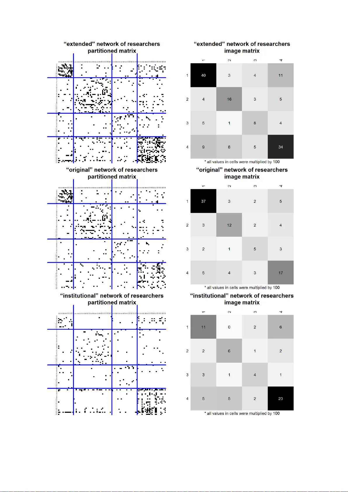
1 NOTICE: this is the au thor’s version of a work that was accepted for p ublication in Socia l networks. Changes resulti ng from the publishing process, such as peer review, editing , corrections, structural formatting, and other quality control mechanisms m ay not be reflected in this d ocument. Changes m ay hav e been made to this work since it was submitted for publication. A definitive version was subsequently publi shed in Social networks, v ol. 39, no. 1, pages 46 – 61 (Oct ober 2014), DOI : http://dx.doi. org/10.101 6/j.socnet.2014.0 4.002 Bl oc k mo d e li n g o f m ul t il evel n e t w or ks Aleš Žiberna * University of Ljubljan a Abstract The ar ticle presents several app roaches to the blockmodeling of multilevel network dat a . Multilevel network data con sist of n etworks th at are measured on at least two levels (e.g. between organizations and people) and information on ties between th ose level s (e .g. information on which people are members of which organizatio ns). Several appro ache s will be considered: a separate analysis of the levels; transfo rming all net works to one lev el and blockmodeling o n th is le vel u sing info rmation fro m al l level s; and a truly multilevel approach where all levels and ties among them are modeled at the same time. Advantages and disad vantages of these approach es will be discussed. Keywords: multile vel netwo rks, multilevel ana lysis, gen eralis ed blo ckmodeling 1 Introduction In the article several approaches to blockmodeling multilevel networks are presented . First, the type of data that are referred to here as multilevel networks will be introdu ced, followed by an explanation of the p roblem that the blockmodeling of multilevel networ ks ( “ multilevel blockmodeling ” ) should s olve. Multile vel net works are composed of one-mode networks (possibly multi-relati onal) for each mode and two- mode networks that “join” units from different levels. * Aleš Žiberna, Faculty o f Soc ial Sciences, University of Ljub ljana, Kardeljeva ploščad 5, 1000 Lju bljana, Slovenia; E-mail: ale s.ziberna@fdv.uni -lj.si ; ales.ziberna@ gmail.comi 2 The goal of m ultilevel blockmodeling is then to find a blockmodel (groups and ties among them) for all these networks simultaneously, namely to partition the units at all levels into groups by taking all available information into account and determin ing the ties among these groups. Three general approaches are presented : a separate analysis of each mode and a comparison of results ; conversi on of the multilevel probl em to a classical one-level block modeling problem; and a true multilevel approach. The suggested approaches are applied to a specific example. At the end of the article, the advantages and disadvantages of the suggested approaches are discus sed. 2 Multilevel netwo rks Multilevel networks can be defined in several diff erent ways . The docu ment “What Are Multilevel Networks ” prepared by the Multi-level Networ k Modeling Group (MNMG) (2012) identifies four different definitions of multil evel networks or multilevel approaches to the analysis of net works. In this articl e, the fourth definition is u sed, namely the one where ties between units at each level are s tudied together with ti es between levels. Therefore, multilevel networks are defin ed here as networks composed of one -mode networks (possibly multi-relational) for each mode and two- mode networks that “join” units from different levels. While most (if not all) multilevel networks are also multi -relational, these two concepts should not be confused. Units in a multilevel network are composed of different types o f units, where each type corresponds to a level . On the other hand, a multi-relational network is a network where several relation s are measured on one (or more) sets of units. Let me first introduc e som e notation:    󰇝           󰇞 is a set of all units and n is the number of all units.  U can be partitioned into L distinct sets (usually two) that represent different levels, so that        and        , for each    .  Each level has         units,   󰇟   󰇠  R is a set o f K relations , where relations are denoted by      󰇟   󰇠  and are measured on units U .  Relations can be defined on all levels (on units from all sets) or on only some levels or combinations of levels.  A multilevel multi-r elational netw ork is denoted b y N = ( U, R ).  O ne -mode networks are denot ed by    󰇛     󰆒 󰇜 , where   󰇟   󰇠 and    . If only certain relati ons are used, this is indicated b y superscri pt.  Two -mode networks are denoted by            󰆒  , where   󰇟   󰇠 ,   󰇟   󰇠 ,    and    . If only certain relatio ns are used, this is ind icated by superscript.  The relation   is repres ented by a v alued matrix   with elements      , where value    indicates the value ( or weigh t) for the arc from unit i to unit j on relation k . 3  Each matrix      󰇟   󰇠 can be partitioned into matrices    , where the first and second dimensions correspond to sets of units/levels. If a relation   is not defin ed from set   to set   then all en tries of submatrix    are undefined 1 .  Several relations ar e represented by three-way arrays       (this is essentially the same as the multiway matrices from Borgatti and Everett, 1992) , where the included relations (   and   , …) ar e lis ted in superscript. If all relations between relati ons   and   are included, this can be written as      . Such arr ays can b e partitioned according to lev els in the same wa y as matrices representing single matric es.  The whole multil evel network N can be r epresented b y a three-way array     .  The relations can be binary, valued, signed or any other kind for which an appropriate blockmodeling app roach is defined. The blockmodelin g approach used to blockm odel a certain relati on must be applicab le to such a relation. While all the methods suggested here can in theory 2 be used on any number of levels, I limit myself to two levels in the whole example section and some other parts of this article. In those parts, I always explicitly state that I am discussing the two -level case. Most of the discussion in the article is limited to the case where two- mode networks represent partitio ns of “ lower ” level units int o “higher” level units, that is each “l ower” level unit is ti ed t o exactly one “higher” level unit, while each “higher” level unit is tied to at least one “lower” level unit. The methodology suggested here is suit able f or all types of two -mode networks, alth ough especially the discussions on reshaping networks and modeling two-mode networks are largel y conditional on this assu mption as the most likel y case in a multil evel context. When I limit the discussion to two -lev el networks, I also limit myself to the case with only three relations. Therefore, I restrict the discussion to the case of a two-level, three-relational network, where relation   is defined on set   (a set of individuals), relation   is on set   (a set of institutions) , and relation   from set   to set   . The multilevel (and multi-relational) network N is repr esented b y matrix R that can be split into the follo wing defined 3 submatrices: o submatrix    , representing the o ne-mod e network of individuals/first-level units    󰇛      󰇜 o submatrix    representing the one-mode network of institutions/second-level units    󰇛      󰇜 o submatrix    , a t wo -mode (affiliation) network tying individuals to institutions / ties between first- and sec ond-level un its      󰇛         󰇜 1 In our implementation they are coded as 0, although th is is irrelevant since they are ignored in all computations. 2 In practice, the time complexity of the algorithm and th e complexity of the nu merous “interactions” between levels would prohibit the application of the method to many levels (e.g., more than 3 or 4). 3 Matrices whose entrie s are defined. The remaining mat rices                                     are undefined (in p ractice coded as 0 matric es). 4 To the best of my knowledge, Iacobucci and Wasserman (1990) were the first to suggest the analysis o f such netw orks and they soon (Wasserman and Iacobucci, 1991) also presented a method for the statistical modeling of such networks. The imp ortance of a multilevel view was later advocated b y Brass et al. (2004). H owever, I am aware of only one example of a multileve l network dataset, the one gathered and analyzed by Lazega et al. (2006, 2008, 2013) . Recently, exponential random effects m odels were also extended to mul tilevel networks (Wang et al., 2013), where they used the same dataset to demonstrate the importance of the method. The same dataset is also used here in th e example secti on . Additional methods (e .g. Snijders et al., 2013) and applications (e.g. Bellotti, 2012; Snijders et al., 2013) can be found for combinations of only one-mode networks at o ne level and a two - mode network connecting this level to another level. Such networks can be seen as a special case of multilevel n etworks as defined here where no relations are collected for one level. 3 Blockmodeling an d some of its exten sions Blockmodeling aims to partition network units into clusters and, at the same time, to partition the set of ties in to blocks (Doreian et al., 2005a, p. 29). Blockmodeling can be also b e “[v]iewed as a method of data reduction, […] a valuable technique in which redundant elements in an observed system ar e reduced to yield a simplified model of relationships among types of elements (units) ” (Borgatti and Everett, 1992) . There are several approaches to b lockmodelin g, such as stochastic b lockmodeling (Holland et al. , 1983; An derson et al., 1992; Snijders and Nowicki, 1997), conventional blockmod eling (e.g. Breiger et al., 1975; Burt, 1976; see Doreian et al., 2005a, pp. 25 – 26 for definition) and generalized blockmod eling (Doreian et al., 2005a, 1994). While this article focuses o n generalized block modeling (Doreian et al., 2005a), mor e precisely ho mogeneity bl ockmodeling (Žiberna, 2007) , at least the first tw o suggested app roaches (se parate analysi s and conve rsion to on e-level block modeling) c an be easily implemen ted using o ther approaches. Some additional no tation is introduced h ere:    is a cluster of units for 1  i  m, where m is the nu mber of clust ers.    󰇝          󰇞 is a partition of the set  ;        ;           .   󰇛     󰇜 is the value of a criterion function that measures the fit of partition C and equivalence E to network N . E can be expressed in different terms, e.g. allowed block types, a pre-specified image etc. (see Doreian et al., 1994 for a further discussion ) but it m us t also include the type o f blockmodeling (e.g. binary, sum of squares etc. – see Žiberna, 2007 f or a further discussion) . In generaliz ed blockmodelin g the criterion function in optim ized when searching for the optimal C given the E and N. A computation of the criterion function for single-relationa l networks is described i n works presenting diff erent approaches to g eneralized blockmodeling (e.g. Doreian et al., 2005a; Žib erna, 2007) . 5 In the remainder of this section, I present several extensi ons to generalized blockmodeling that are required for the approaches suggested in the next section, especia lly for the true multilevel approach, although their usefulness extends well beyond their application to multilevel block modeling. 3.1 Multi-relational blockmodeling Although (classical) blockmodeling was initially developed fo r multi -relational networks (Breiger et al., 1975; Burt, 1976 ; White and Reitz, 1983; White et al., 1976), generalized blockmodeling was only developed for single relatio ns. While Doreian et al. (Doreian et al., 2005a; Ferligoj et al., 1 996) discussed m ultiple relations among possible extensi ons to generalized block modeling in their book (Doreian et al., 2005a), they did so with s erious reservations. Recently, Brusco et al. (2013) presented multi-objective blockmodeling that can be used to blockmodel multi-relational netw orks. Even though their approach is most likel y more appropriate, a simpler app roach is used her e. The extension of generalized blockmodeling to multiple relations is at least in technical terms straightforward. Generalized blockmodeling is an optimization approach that searches for the optimal partition by minimiz ing the criterion functi on. We could sa y that in the ca se of multiple relations this turns into a multi-objective clustering problem (Ferligoj and Bat agelj, 1992) (a criterion function for each relation presenting one objective). One possibility that will be used in this article is to transfor m this multi-obje ctive problem to single-objective problem using the weighted sum approach (E hrgott and Wiecek, 2005; Ferligoj and Batagelj, 1 99 2) . Several issues arise when using this approach, from ch oosing suitabl e weights to purely conc eptual proble ms; however, these issu es exceed the s cope of this article. The criterion function for m ulti-relational network N with K relations can be computed as follows:  󰇛     󰇜                  where     is a weight for relati on      󰇟   󰇠 ( 1 ) As mentioned, the multi-objective approach (Brusco et al., 2013) might be more appropriate than the weighted sum approach, but I have currentl y not yet implement ed it in my software. 3.2 Different sets of uni ts In multilevel blockmod eling we have several sets o f units (at least tw o), one for each level. These sets of units must be partitioned separatel y, that is units from different sets cannot be together in the sa me cluster. 6 Le t us define the set of fea sible partitions  as :      󰇌                                , where   is a partition of the set   ,    is the  -th cluster of the partition   and   is the number of clusters in the partition   .           ( 2 ) The probl em can be expressed as a constrained clustering problem (Batagel j an d Ferl igoj, 1998; Gordon, 1 996) .  󰇛       󰇜     󰇛     󰇜 ( 3 ) Such a restriction for two sets is already used in two -mod e blockmodeling (e.g. Doreian et al., 2004). For multile vel blockmodelin g such a restri ction m ust be ex tended to single -mode networks and more than two sets. The usability of such restrictions goes beyo nd multilevel blockmodeling. It can be used always when distinct sets of units exist that either should not be mixed or we believe that the optimal partition will no t have them mixed. When this restrictio n is used, this reduces the neighb orhood that must be searched in either a local search or similar algorithm, thus redu cing its time complexity. For example, such a restriction could be used when analyzing a baboon grooming network as was done by Doreian et al. (2005a, 2005b) since baboons of differ ent genders ne ver appear in th e same cluster. 4 Multilevel blockm odeling The ultimate goal of multilevel blockmod eling is to find a blockmodel (groups and ties among them) for the whole m ultil evel network, which is to partition the units at all levels into groups by taking all available informati on into account and d etermining the ties among these groups. In this article, thre e genera l approaches are dis cussed: a) a separate analy sis of each mode and a comparison of the results; b) conversion of the multilev el problem to a classical on e-level blockm odeling pr oblem (hereafter “ the con version approach ” ); and c) a true multilevel app roach. These are not reall y alternative approaches since at least the first one (sepa rate analysis) should be the first step in any blockmodeling analysis of multilevel networ ks. The separate analysis approach (a) represents a good exploratory technique and can guide a m ore comple x analysis and show whether more complex appr oaches are even justified. The conversion s approach (b) is appropriate when we want to focus on a certain level while using information from the other level(s) to improve the partition and/ or when the other level(s) can be used as 7 indirect relations for units of the level in focus. In contrast, the multilevel approach (c) should be used when we already have some knowledge about the network ’s structure . It can provide us with a n ovel in sight in to the ties a mong clusters from different le vels. It can also help us search for such clus ters at ind ividual levels in such a way that the ties amon g them are relatively “clean”. In addition, the m ul tilevel ap proa ch can ha ve si milar effects as th e conversion approach since information from one level is used to better determi ne clusters on the other level. Us e of the first and at lea st one of the other two a pproaches is also in line with the idea of Lazega et al. (2013 ) that it “is important t o examine b oth levels separatel y and jointly”. 4.1 A separate anal ysis of each mode and a comparison of the results The simplest way to analy ze a multilevel network using blockmodeling is to blockmodel each level separately and then compare th e results. The comparison can be done in se veral ways: a) forcing the partition obtained at o ne level o nto the o ther leve l(s) and analyzing the fit ; or b) obtaining the par titions on all lev els and comparing them. Both options are complementary and preferably bo th should be us ed. The first option in (a) means that, after obtainin g a partition on a given level, this partition is forc ed onto an other level. This can be done by either reshapin g the partition to the level on which it is to be forced or reshaping the one -mode network of the level o n which the partition is to be forced to the level on which the partition was obt ained. B oth reshapings are done through the use of th e two -mode netw orks joining the t wo levels. The more detailed description that follows applies to the case o f a two-level, three-relational network. The reshapin g is most s traightforward when the two-mode network essential ly represents a partition o f units of the first level into classes defined by the second level and we are reshaping the second-level parti tion to the first level. In such cases, the second-level partition can be reshaped to the first level sim ply by assign ing to the units of the first level the class (cluster) of the un its of the sec ond level to which these units bel ong. Similarly, we can e asily reshap e the network of the se cond level to the first by assigning the tie of the second-level units to pairs of first-level units that are associated with these second-level units. This can be simply obtained by pre- and post-multiplying the matrix re presenting the second-level network by the matrix representing the two-mode network (tra nsposed when needed) as presen ted in Equation ( 4 ).                   󰆒      ( 4 ) The reshap ed net work      󰇛      󰇜 actuall y represen ts ind irect ti es between units o f the first level through the ties among sec ond-level units to which these first-l evel units are associated. Such a transformation is also undertaken by Lazega et al. (2013) where they call neighbors in such a resulting netw ork “dual actors”. 8 The transformations are a little more complicated in the other direction or when first-level units are tied to more than one second-level unit. In such cases, some averag ing, voting or aggregation rules are required 4 . After a partition at one level is obtained and a suitable reshaping has been applied, we can see how this partiti on fits the other level. That is, we can check whether the pattern of ties of the second network is well explained by this partition and therefo re by the struct ure o f the first- level network. We could say that we are performin g a kind of pre -specifi ed blockmodeling (Batagelj et al., 1998) and checking the fit o f the pre-specified partition (and possibly a blockmodel image) to a network. If the fit is good (significantly better than random), we can say that the structures of both networks are associated. In addition, we can check whether the blockmodel images are similar at both l evels. If they are, this indicates that n ot only are the groups on one level associated with the groups on the o ther level, but so too is the pattern of ties among groups. The sec ond opti on (b) is to compare partiti ons o btained at both le vels. This is done by reshaping one of the partitions for it to be compatible with the other and using some classical indices fo r comparing partitions to compare them, such as th e Rand Index (R and, 1971) or Adjusted Rand Index (ARI) (Hubert and Arabie, 1985). Obviously, larger values of these indices indicate a stronger association among the partiti ons and theref ore among the gl obal structure s of th e o ne-mod e ne tworks at diff erent levels. All value s of ARI over 0 indicate that the association is great er than would be expe cted by chance. Sinc e this approach is a good exploratory technique, it is simple to perform and allows an estimation of the association of group structures across levels, it should always be the first step in the analysis. These comparisons allow us to determine whether there is so me similarity in the structure of the two networks and whether the similarity is only in the partitions or also in the pattern of ties among groups. Where no similari ty is found, more complex analyses are probably not justified. In case of only partition similarities, the single-relational version (explained in the nex t subsecti on) of the conversi on approach is most likely un suitabl e. Of c ourse, this approach also has limi tations especially since all par titions are on ly based on one le vel and that the ties between g roups of different levels cannot be modeled, only observed. However , this does not li mit its usefulness a s an exploratory technique. 4 For exampl e, if a first -level unit belon gs to s everal secon d-level un its and we want t o reshape the second-level partition to the first level, there is a prob lem of what class to assign to this first -level unit if all the second-level units have different classes. One p ossibility is to assign a majority class if such a class exists, to randomly select on e class, or to create a new cl ass for each uniq ue co mbination of classes of the affiliated second- level units. Similarly, the reshaping of th e network in such a case requires some aggregation principles to determine the presence or value of ti es in the reshaped n etwork. For valued networks, sum, average, mini mum or maximum are possible aggr egating functions, wherea s wh en a binary network is used some threshold could be supp lied to determine at what density of ties in th e subnetwork of second -level un its the tie would be form ed in the re shaped network. As this exceeds the s cope of thi s p aper, any more detailed discussion is omitted. 9 4.2 Conversion of the multilevel problem to a classical one-leve l blockmodeling pr oblem The first approach suggested here that takes information about all lev els into account is to convert this multilevel problem to a on e-level problem. The approach is appropria te in cases where we believe that the partitions at different levels are practically the same (after reshaping) and we want to u se as much information as possible t o find these partitions. In fact , when using this approach only a partition at o ne level is obtained (the “ m ain ” level), which can then be reshaped if desired to o btain partitions at “other” 5 levels 6 . Therefore, we should o nly use it if we find in the separate analysis stage that the partitions for all levels are similar or if that one partition a t least app roximately fits all levels . In this approach, we there fore reshape the network from “other” levels to the “main ” level and then partition all networks at the main level simultaneously. The resha ped netw ork s represent add itional (indir ect) relations 7 in the “ main ” level ’s netw ork. If, in the case of two levels, we reshape    into    as was presented in the previous subsection, the “joint” multi- relational networ k is                         . We have two o ptions when analyzi ng the obtained multi-relational network. The first one is to somehow aggrega te these relations by using so me function like maxi mum (other options include minimum, average and sum) on relations on the same tie. This op tion only really makes sense if all network s measure similar concepts and have a similar structure in te rms of both the partitions and patterns of ties a mong groups. For exa mple, if we can consider one network person ’ s direct access to some resou rces and the other network person’s indirect access through institutional exchange. In some cases, it might be sensible to find a partition at one le vel usin g this approach, but not on the other. E.g. it might make sense to assume that employees can access resources throug h their firm’s connections, but not vice versa 8 . In this case, when partitioning the employees it would be sensible to include their firms’ connections to better estimate their position in some network, but it would no t make sense to esti mate the firms ’ positions also usin g th eir employees’ connections. 5 Other than th e “main” level, that is other than the one to which all network s were reshaped. 6 In the th eoretical part, if not explicitly stated I otherwis e discus s the more general case where there can be two or more levels. This means that there can be one or more » other« levels and therefore either singular or plural form are app ropriate. I will however use the p lural form with the understanding that in the case of just two levels there is only one “oth er” level. 7 In the case where the netwo rk to be reshaped is multi -relat ional, we also o btain sever al relations by reshaping each relation separately. 8 I do not im ply that firms can (never) access resou rces through employees’ (per sonal) networks. 10 The second option, which is usuall y more appropriate, is to blockmodel the multi-relational network directly using the multi-rela tional blockmodeling discussed in subsection 3.1 . This simply m eans that we perform blockmodeling on all relations simultaneously by constraining them to the sa me partition using Equ ation ( 1 ) . In the t wo -level case, the criterion func tion used is then:               󰇛        󰇜                ( 5 ) The advantages of this approach are that it is still relatively simple to perform and that it uses all available informati on (on all) levels to o b tain a partition at the selected (“main”) level. However, as discussed above, this only makes sens e in certain cases. The ap proach also has several disadvantages, the first being that some information is lost in the aggregation, especially if the single-relational approach (aggregati ng relations prior to the blockm odeling analysis) is used. Second, the choice o f suitable weights can be problematic when a multi- relational version is used. Finally, the approach obtains just one 9 partition that is then reshaped to different levels. This m eans that th e tie s between gr oups at differ ent le vels are fixed and cannot be observed or modeled. The “other” levels’ partitions are a function of the original partiti on obtaine d at the “main” level an d the tw o-mode networ k(s) joining the “other” levels with the “main ” level. 4.3 The true multilevel approach The purpose of this approach is to partition units of all levels simultaneously (using multi- criteria clustering) by takin g account of both the ties within l evels and those between levels (two-mode network(s)) . Formally for the two-level, three-rela tional case (network   , networ k   and network   ) this means finding partitions   (of set   ) and   (of set   ) that optimize the foll owing criterion functi on:  󰇛                        󰇜     󰇛         󰇜     󰇛         󰇜     󰇛            󰇜 ( 6 ) A more general approach (not adapted to a certain number of levels or relations) is to join all one-mode and two-mode netw orks into a single multi-relational netw ork 10 N (also represented by three-way array R ) as introduced in Section 2 . In this case, the criterion function is sim pl y 9 We could use d ifferent levels as a » base« level, th at is the level to which other le vels are reshaped. The partitions obtained u sing different base levels might then slightly differ when reshaped to the same level, e specially if in th e t wo-mode network units from both sets of nodes can have many ties (to nodes of the other set). 10 Although in some applications it might be possible to treat the whole multilevel netw ork as a one- relational network, this i s re latively unlikely as most likely one -mode networks on different levels an d the two-mode network(s) will measure different relations in the majority of applications. Therefor e, the more gen eral an d probable situation wher e the multilevel network is also multi -relat ional will b e considered here. 11 the criterion function for multi-relational blockmodeling (Equation ( 1 )) with the constrain t that each level is partitioned separatel y (Equation ( 3 ) ). 4.3.1 Specifying equival ences for part s of the mult ilevel networ k As can be seen from Equa tion ( 1 ), we need to specify equi valence for each relation. Each relation is usuall y defined only on one set/level of units (single-le vel one-mode ne twork) or only between two sets o f units (two -mode networks). For parts of the network where the relations are not defined, the only allowed block type should be a “Do not care” block (Doreian et al., 2005a, p. 235) . The inconsistency o f such a block is always zero (regardless o f the ties in the block). This ensur es that only appropria te parts of the r elations/network or in technical terms of the thre e-way a rray R are taken int o a ccount when computing th e value of th e criterion functi on. For these parts of relations that are defined, that is for each o f t he one-mode and two-mode networks separatel y, we can specify suitable generalized blockmodeling approaches, allowed block types and possibly their positions (or equivalences). Suitable specifications for one -mode networks can be found in the relevant lit erature (e.g. Doreian et al., 2005a; Žiberna, 200 7) . While generalized blockmodelin g of two-m ode networks has also been covered (Doreian et al., 2005a, 2004), so me aspects specific to its use in multilevel bloc kmodeling are dis cussed here. In most cases it will be desired that most blocks in the two -m ode network are null (empty, without any ties) since this makes the connections between the groups at different levels clearer. Preferably, such blocks wo uld have no incons istencies (no ties). The way of obtainin g such null blocks depends on the blockmodeling approach applied. Using some approaches ( lik e those shown in the example in Section 5.4), almost perfect null blocks in two-mode networks can be obtained by usin g structural equivalence and simply giving a large weight to the two- mode network criterion function. The goal of very few or even no inconsist encies in null blocks can be achieved by heavily penalizing the inconsistencies in the null blocks as e.g. in Dorei an et al. (2005a, pp. 260 – 261) . However, sometimes we might a lso want to impose restrictions in terms of pre-specified bloc kmodels (Batagelj et al. , 1998) or allowed images, e.g. that each row (i.e. level one) cluster might be associated with only one column (i.e. level two) cluster. A further discussion of possible restrictions can be found in Appendix A. In the case of two levels when equivalences for two-mode netw orks ensure (at least approximately) that each lower level cluster is tied (actua lly the units it contains) to only one higher level c luster and vice versa, this restricti on is similar to the restriction im posed by the multi-relation al conversion approach (see Appendix A for details) and we therefore expect these approaches to produce similar results (of course, provided that equivalences for the one-mode n etworks are also specified in the sa me way for the two approaches ). 4.3.2 Advantages and d isadvantages of t he true multil evel approach The true multilevel approach has several advantages, namely that it takes all available information (all o ne-mode and two -m ode ne tworks) into account, that n o aggregation i s necessary, and that ties between levels can be modeled. However, it also has several drawbacks. In conceptual terms, the main disad vantages are that there are no clear guidelin es concerning what are appropriate restricti ons for ties between levels and what are appropriate 12 weights for different parts of multi-relational networks, that is for level-specific one-mode networks and for the two-mode netw orks. In the even t of equal weights, in principle the parts with larg er inconsist encies hav e a bigger influence on the results. As the inconsistencies are dependent on the equival ences (or allowed bl ock types and their positions), netw orks ’ size, pattern of and number of clusters, all these factors influence the appropriat e weighting . A suggestion that is als o followed in th e example in subsection 5.4 is to make the weights reciprocally proportional to the inconsis tencies of the relations/single-relational network if the whole network (for which the relation is defin ed) would be in a single block (that is, if all units (from the same mode/level in two-mode networks) would be in the same cluster). If we want very few inconsistencies in the two -m ode network( s) , this/these network(s) can be given higher weight(s) (e.g. double the one computed based on the suggestion in this paragraph as is also used in the exa mple). Additional disadvantages are tied to o pti mizational problems, especially as a local search wit h a single exchange and move as allowed “moves” is currently used for optimization. Finding an optimal partition using the direct approach is in most cases an NP -hard problem (Batagelj et al., 2004, p. 461). The mul tilevel app roach is even more ti me-demanding as there are more units in a multilevel network than in single-lev el networks. However, the main problem lies in the fact that currently a local search with allowed transfor mations being a single exchange and a single move is used (see e.g. Batagelj et al., 1992, p. 127 for details). This is problematic since in the multilev el approach quite hard constraints are usually desired fo r a two -mode network(s), typically by desiri ng null blocks and strongly w eighting the inc onsistencies in the two -mode network(s) (at least those in the null blocks) 11 . If the current partition is such that ties between a certain higher level unit and some lower level units are in a non-null block, moving just the higher level unit (since only o ne move at a time is allowed) would most likely move several ties in the two-mode network to the null block and would therefore be very costly 12 , to a such an extent that the move would most likely not be selected. In the current implementation, I attempt to circumvent this proble m by applying two strategies. The first one is brute for ce, namel y by using many rando m star ting partitions with a local s ea rch. The second o ne is not to weight inconsistencies in the two-mode network(s) too strongly 13 in the first stage in order not to make such moves too costly. If this results in an und er-structured two -mode network(s) (too many ties in the null block or too few null blocks), the resulting partition can be further optimized with more stringent constraints on t he two-mode network(s), namely by increasing the weigh t of the inconsistencies in the two-mode network(s). Of course, it would be better to use an adapted tabu search (Brusco and Steinley, 2011) or similar algorithm that would temporarily allow costly moves or direct multiobjective blockmodeling (Brusc o et al., 2013 ) . 11 Meaning that an additional tie in th e null block of th e two - mode network increases the inconsistency by much more than the inconsistency in th e one-mode n etworks 12 Meaning that th ey do not increase the incon sistency too much 13 E.g. to use weights compu ted as suggested in the p revious paragraph 13 5 Example: Applic ation to a mul tilevel network of elite cance r researchers in Fr ance The suggest ed approach is demonstra ted o n a mu ltilevel net work o f th e elite of cancer researchers in France (Lazega et al., 2008). The analyzed multilevel ne twork is composed o f two levels, a le vel of re searchers an d a level of res earch labs. The networks and other data used are des cribed in more detail in the following subsection. General ized blockmodeling offers a wide range of possible analysis. Due to space limitations and the focus on the method (not the application) of this article, only one possibili ty is presented here. An attempt is made to find cohesive groups and determine whether they are associated with certain researchers ’ or labs’ specialti es. To achieve this, generaliz ed blockmodeling with pre -specifi ed blockmod eling was used. The pre-specified block model correspondin g to cohesive groups was used fo r one-mode networks , namely by only allowing “null” blocks in off - diagonal blocks and only “complete” blocks on the diagonal blocks within each level and/or relation. Several approaches to generaliz ed blockmodeling exist (Doreian et al., 2005a; Žiberna , 2007 ). Hom ogeneity blockmodeling wi th sum of squares (SS) blockmodeling according to structural equivalence was used here in all the analyses for all levels and relations. However, it should be emphasized that ther e is no need to use the same approach for all levels/relati ons. In order to prevent null blocks from appearing where complete blocks are required (on the diagonal) and to prevent almost null blocks from being classified as complete, the constrained version of complete blocks as described in Žiberna (2013a) was used. That is, the value from which sum o f square d eviations were computed was constrained to a pre-specified value, which was set to twice the m ean of the relation/level. As a local search is used to find the “optimal” partition, at least 1,000 random starting points were used in all analyse s. All of the analysis was performed using the development version of blockmodeling 0.2.2 package (Žiberna, 2013b, 2013c) within the R 3.0.1 software environment for statistical computin g and graphics (R Co re Team, 20 13) . 5.1 Data description The suggested approaches were app lied to the multilevel n etwork of the elite o f cancer researchers in Fran ce gat hered and anal yzed b y La zega et al . (Lazega e t al., 2013, 2008) . Several networks of researchers and several network s of labs were collected together with a two -mode network of researchers ’ membership in laborat ories (labs). For this demonstration, the same kind of aggregation as perfor med by Lazega et al. (2008) was used. This gave us the foll owing networks : o a network of res earchers o a network of labs o a t wo -mode network of labs and researchers: A m ember ship matrix of labs x researcher s In this application I am usin g data on 78 labs and 98 researchers, namely all cases where I had data on pairs of researchers and labs (or larger groups since there can be more than one 14 researcher per lab). While some labs and researchers have no outgoing ties, they were not excluded since the y were nomina ted by others. First, both networks (and the ties between the m) are presented graphically i n Figure 1 and Figure 2. Little can be learned from these two representations except that the network of researchers is denser and perhaps has more structure. Table 1 re veals im portant difference s between the networks. Th e reciprocity and to a lesser extent clustering coefficient are larger in the network of researche rs network than in the labs network. This might indicate that blockmodeling analysis might more appropriate for th e network of res earchers as there is more “grouping” in this network. Out -degree centralization and betweenness centralization are larger in the network of labs. The high o ut-degr ee centralization is the result of t wo labs reporting many more ties than other labs. Based o n this, we cannot expect a similar structure in both networ ks and especially no t the same bl ockmodels and equivalences, yet we c annot rule o ut some similarities in structure such as similar partitions, same equivalence s with different blockmod els (image ma trices) etc. Lazega et al. (2008) reported several variables measured on researchers and labs, however only specialties of researchers and labs (5 binary variables for resear chers and 5 for labs) are used here for validati on purp oses . R es Labs Size 98 78 Density 0.059 0.039 Average in-degree 5.745 3.013 Centralization – degree 0.139 0.220 Centralization – in -degree 0.117 0.1 18 Centralization – out-degree 0.190 0.381 Centralization – betweenness 0.122 0.244 Clustering coefficient 0.266 0.184 Reciprocity 0.367 0.083 Table 1: Basic network statistics Figure 1: Graph ic representation of the whole (multilevel) network – rese archers are up /right, labs are down/left 15 Figure 2: Matrix representation of the whole (multil evel) network – researchers are up/left, labs are down/right To estimate the overlap o f the network of research er and network of labs networks the network of labs was reshaped to fit the network of researcher s. This reshaped network o f labs is actually a network among researchers where a tie between two researchers means that their labs are tied. The overall o verlap measured as the percentage of researchers’ ties that have “support” in the network of labs is 29 .2%. If we take the opposite direction and reshape the network of researchers to labs by creating a tie between two labs if at least some researchers from those labs are connected and compute the overlap as the percentage o f labs’ ties that have “support” in the network of researchers we obtain 18 .1%. However, here we are focusing on the first case where we are mainly interested in the support for the resea rchers’ ties in the network of labs. Another way to assess the tie similarity of the networks is through the associati on coefficient Cramer's V, which is 0.216 for the network of researchers and the r eshaped network of labs. Th e small overall o verlap and small association coefficient indicate that the networks are quite different. While it is possible that some common structure is present in both networks, it is not very likely. Especially the image matrices are expected to be v ery different. 5.2 Separate analysis The first and simple st way to analyze multile vel networks is to analyze each level separately and then compare the results. While this is the simple st anal ysis, it can provide relatively rich results especially in terms of similarit y of structure and sh ould always b e the first step of th e analysis. 16 5.2.1 Network of resea rchers As mentioned, cohesive groups are first search ed for in the networ k of researchers. The pre-specified value was set to twice the density, namely to 0.12. As the appropriate number o f clusters is not known, t he number of clusters from 2 to 8 was tested and the corresponding errors are presented in Figure 3. Networks/ matrices partitioned according to solutions with 4 to 7 clu sters are presented in Fi gure 4 . I excluded partitions with less or more clusters based on the desir ed level of complexity and results in Figure 3. Based on Figure 3 and Figure 4, the most appropriate number of clusters is 4, 5 or 7 clusters. I opted to present the 4 -cluster solution as the least complex one. The same procedure for determining the appropriate number of clusters was used in the analysis of the networks of labs and in the conversion approach (presented in Section 5.3), although there the figures similar to Figure 3 and Figure 4 are omitted and only the network partition according to the s elected number of clusters is pres ented. Figure 3: Errors for SS blockmodeling of the network of researchers using a cohesiv e groups pre-specified blockmodel by different numbers of clusters The image in Figure 5 represents the densities of the resulting blocks. We can see that we have two more “ cohesive ” clusters ( 1 and 3 ) and two less “ cohesive ” ones (2 and 4). In Table 2 we explore if this partition can be associated with exogenous variables. We can see that the more cohesive clusters according to the block model are also more homogeneous according to the researcher s ’ specialties, as 91% of research ers from cluster 1 list “ fundamental research ” among their specialties and 92% of res earchers fr om cluster 3 list “ hemat ology” among their specialties. Yet this is not always the case as e.g. in the 7-cluster partition some clusters are relatively homogeneous according to specialties (n ot presented here) and n ot according t o the blockmodel and vic e versa. 5.2.2 Network of labs The same procedure applied to the network o f researchers was also applied to the network of labs. The pre-specified value wa s again chosen to be twice the density, that is 0. 08 . The number of cluster s from 2 to 8 was tested and the 3-clu ster s olution was selected. The partitioned networ k and corresponding image are presented in Figu re 6 . The densities in the image show that the c ohesive groups ’ model does not fit and a more core -perip hery-like structure emerges. However, enforcing a core-periphery structure does not produce satisfac tory r esults. As this exam ple is only used for illustration I do not exten d it further. In Table 3 we explore if this partition c an be associated by 17 exogenous variables, but no clear association can be found, although some differences among clusters do exist. Figure 4 : The network of researchers partitioned using SS blockmodeling with a cohesive groups pre-specified blockmodel 5.2.3 Comparison Here the partitions obtain ed on both level s are compared. To facilitate the comparison, the labs ’ partition is first expanded to researchers (each researcher is "assign ed" the cluster of their lab). The 2 to 8 cluster lab s’ partitions were compared to the 2 to 8 cluster researcher s’ partitions using the Adjusted Rand Index (ARI) (Hubert and Arabie, 1985) . All ARIs were close to 0, the highest being 0. 20 for an 8 cluster researchers ’ partition and 4-cluster labs ’ partition. Therefore, the association there among partitions based on different levels is low. This does not give much hope with regard to more complex analyses. 18 Figure 5: Image of the 4-cluster partition for the network of re searchers SS partition using a cohesive groups pre-specified blockmodel 1 2 3 4 All frequency 12 45 12 29 98 res - solid tumors 0.45 0.56 0.17 0.38 0.44 res - hematology 0.18 0.16 0.92 0.28 0.29 res - surgery 0.00 0.18 0.00 0.00 0.08 res - public health 0.36 0.20 0.00 0.03 0.14 res - laboratory rese arch 0.73 0.36 0.25 0.62 0.46 res - fundamental r esearch 0.91 0.22 0.50 0.59 0.44 lab - solid tumors 0.55 0.30 0.18 0.37 0.33 lab - hematology 0.18 0.14 0.45 0.22 0.20 lab - surgery 0.00 0.07 0.00 0.00 0.03 lab - public health 0.00 0.20 0.00 0.07 0.12 lab - laboratory res earch 0.36 0.36 0.36 0.59 0.43 lab - fundamental res earch 1.00 0.45 0.45 0.67 0.58 Table 2: Averages of exogenous variables by blocks for the net work of r esearchers SS partition using a c ohesive groups pre-specified blockmodel There is some similarity in terms of the association am ong the exogenous variables and the partitions. Both the researchers ’ and the labs ’ partition are to some extent associated with specific specialties, although for the net work of researchers these are res earchers' specialties (hematology and solid tumors), while for the lab s these are labs' specialties (fundamental research and s olid tumors). This does giv e some hope for the further analysis. Another way to compare partitions among levels is to use a partition from one level and apply it to another level. For example, we could force the labs ’ partition onto the network of researchers and check the fit. For illustrati on the 3 -cluster labs ’ partition obtained in the previous sub-subsection is forced onto the network of researchers. Like before when computing the ARI, he re we also must first expand the labs ’ partition to the researchers. The ne twork o f r esearchers partitioned according t o this partition and the corresponding image are shown in Figure 7 . The image matrix shows that the 19 densities o f the on-diagonal blocks are larger than those o f the off-diagonal blocks expected for the cohesive g roups mo del; h owever, all are relativ ely c lose to the density of the whole network. Th e error for this model is 542.8, which is relatively close to the “maximal” error of 563 (o btain ed if the whole n etwork is in a single null or complete block) and much further from the optimal resul t obtained in the sub-subsection 5. 2.1, which is 504.3 for the 3 -cluster partition. This ind icates that, while there is some similarity among the structure of both networks, it is v ery small as this error is closer to “maxim al” (and th erefore also a “ rand om” error) than to the optimal on e. Figure 6 : The network of labs partition ed i nto 3 clusters using SS b lockmodeling with a cohesive groups p re -specified blockmodel and the corresponding image 1 2 3 A ll frequency 27 32 19 78 res - solid tumors 0.44 0.58 0.32 0.47 res – hematology 0.26 0.27 0.31 0.27 res – surgery 0.07 0.17 0.00 0.10 res - public health 0.04 0.16 0.32 0.15 res - laboratory rese arch 0.48 0.41 0.56 0.47 res - fundamental r esearch 0.44 0.34 0.61 0.44 lab - solid tumors 0.22 0.53 0.22 0.35 lab – hematolog y 0.15 0.22 0.28 0.21 lab – surgery 0.04 0.06 0.00 0.04 lab - public health 0.19 0.03 0.17 0.12 lab - laboratory res earch 0.52 0.34 0.44 0.43 lab - fundamental res earch 0.52 0.50 0.78 0.57 Table 3: Averages of exogenous variables by clusters for the ne twork of labs SS partit ion using a cohesive groups pre- specified blockmodel. Averages are computed as averages of average lab values among the interviewed researchers. A similar analysis could also be performed for o ther partitions. In the case of applying a researchers ’ partition to the network of labs, reshaping this partition is a little more problematic although several approaches are reasonable. Another option to “ circumvent ” this is to reshap e the network of labs to the researchers which i s less complica ted. Further discu ssion of this exceeds the scope of this article. 20 Figure 7 : The network of researchers partitioned ac cording to th e 3-cluster labs ’ partition using SS blockmodeling with a cohesive groups pre-specified blockmodel and the corre spondi ng image 5.3 Conversion of the multilevel pr oblem to a classical one -level blockmodeling pr oblem In this subsection the multilevel proble m was converted to a one -level problem, namely to a single set of units. In particular, here the netw ork of labs was c onverted to res earchers ’ “spac e” 14 by defining a new relation between researchers based on ties between labs. In this new relation (let u s call it “ institutional ”) two research ers are tied if their labs are tied (o r if they are members of the same lab). Fu rther analysis v aries o n how we combine this network with the “original” netw ork of researchers. The first option is to create a new sing le-relational (“ extended ”) network where two researchers are tied if they are tied directly (“original” network of researchers) o r through their labs (“ institution al ” network). Such networks are also discussed by Lazega et al. (2 013) in terms of extended opportunity structures . Another approach is to combine these two relations into a m ulti- relational networ k (of researchers). 5.3.1 Single-relational netw ork The same pre-specified blockm odel as was applied to the network of researchers in the previous section (“ Separate analysis ”) was applied to this “ extended ” network with only the pre -specifi ed value for constr ained complete blocks (on the di agonal of the pre -specifie d blockmodel) b eing updated to 0.18, the mean of the “ extended ” network. A 4-cluster solution was selected as the most appropriate. The “extended” network of researchers and its “components” ( the “original” network of researchers and the “ institutional ” network of researchers) and the correspondin g images (block 14 Conversion of the network o f researchers to t he labs’ “space” is also po ssible, although more complex. 21 densities) are presented in Figure 8 (partitioned matrices on the left and image matrices on the right) . In Table 4 we can see that the o btain ed clusters differ quite significantly, especially in the rese archers’ special ties . 5.3.2 Multi-relational net work We will again tr y t o search fo r cohesive groups in this multi-relational networ k ( of r esearchers) by imposing a pre-specified cohesive groups blockmodel o n both relations, where the pre -specifi ed value is set to approximately twice the mean of each relation (0.12 for the “original” and 0.09 for the “institutional” relation) . The 4-cluster solution was selected as the most approp riate. Both relations partitioned according to this so luti on and the correspondin g im ag es are pr esented in Figure 9 (partitioned matrices o n the left and image matrices on the right ). The den sities show that the cohesive groups model fits. Moreover, we can see that clusters 1 and to a smaller exte nt 2 are primarily “determined” by the “original” network, while cluster 4 is chiefly defined by the “institutional” network. In Table 5 we can see that the o btained clusters differ quite significantly in specialties. In both approa ches we can notice that almost all re searchers in cluster 1 specialize in hematology, while most o f the labs in which r esearch ers from cluster 4 are employed specialize in fundamental resear ch. 5.4 A true multilevel approach The true multi-relational approach is an approach where w e partition the multilevel ne twork as presented in Figure 1 and Figure 2 . Here a cohesive groups pre-specified blockmodel (the same as in the separate analysis stage) was used on both levels. On the two -mode network linking the two levels SS bl ockmodeling according to structural equivalence with constrained complete blocks was used. The compl ete blocks were constrained by setting the pre-specified value to 0.03 (twic e the density, round ed up wards). This was used to try to give some incentive for the blocks in the two- mode n etwork t o be eithe r (completel y or alm ost co mpletely) null or denser t han the whole two- mode netw ork. What we want is as many completely or nearly completely null blocks as possible to make the comparis on of the researchers ’ and labs ’ clusters easier, although we do not want to force th e researchers ’ and labs ’ clusters to m atch perfectly (e .g. by forcing all researchers from labs from a given cluster of labs to be in the same cluster o f researchers ). Since when using this approach finding the global (and not local) optimum is more problemat ic, at least 10 , 000 random starting points were used (instead of the 1,000 used in the other exampl es). For a true multilevel approach, we have to somehow allow for an appropriate contribution of both levels and of the two-mod e network. In the sugge sted approach, this is a chieved th rough appropriate weighting. I decided to weigh t the relations (that is both lev els and the two -m ode network) reversely proportional to the “worst case” error, that is the error obtained in the case of only one cluster (using the blockm odeling approach s elected for a given relation /level). Therefore, the following weights were used: 1 for the network of researchers, 2.346 for the network of labs and 5.478 for the two -mode network (“ the original”) . In o rder to try to obtain even clear er associations among the researchers’ clusters and labs’ clusters, weights with a double weight for the two-mode network was also tri ed (“double two - mode”). 22 Figure 8 : The “ extended ” network of researchers and its “ compo nents” ( the “original” network of researchers and the “institutional” network of researchers) – partitioned into 4 clusters using SS blockmodeling using a cohesive groups pre- specified blockmodel and the corresponding images 23 1 2 3 4 all frequency 14 35 23 26 98 res - solid tumors 0.21 0.66 0.39 0.32 0.44 res – hematology 0.86 0.11 0.30 0.20 0.29 res – surgery 0.00 0.17 0.09 0.00 0.08 res - public health 0.07 0.17 0.13 0.16 0.14 res - laboratory rese arch 0.29 0.26 0.57 0.76 0.46 res - fundamental r esearch 0.50 0.17 0.43 0.80 0.44 lab - solid tumors 0.15 0.35 0.52 0.22 0.33 lab – hematolog y 0.54 0.09 0.22 0.17 0.20 lab – surgery 0.00 0.06 0.04 0.00 0.03 lab - public health 0.00 0.26 0.09 0.00 0.12 lab - laboratory res earch 0.31 0.32 0.39 0.70 0.43 lab - fundamental res earch 0.46 0.44 0.57 0.87 0.58 Table 4: Averages of ex ogenous variables by bloc ks for the “ extended ” network of researchers SS partition using a cohesive groups p re -specified bloc kmodel Figure 9 : The multi-relational network of researchers partitioned using SS blockmodeling usin g a cohesive gr oups pre- specified blockmodel and the corresponding images 24 1 2 3 4 all frequency 14 34 29 21 98 res - solid tumors 0.14 0.53 0.55 0.35 0.44 res – hematology 0.93 0.12 0.21 0.25 0.29 res – surgery 0.00 0.18 0.07 0.00 0.08 res - public health 0.00 0.09 0.24 0.2 0.14 res - laboratory rese arch 0.21 0.38 0.48 0.75 0.46 res - fundamental r esearch 0.50 0.26 0.34 0.85 0.44 lab - solid tumors 0.15 0.24 0.55 0.28 0.33 lab – hematolog y 0.54 0.00 0.21 0.33 0.20 lab – surgery 0.00 0.06 0.03 0.00 0.03 lab - public health 0.00 0.27 0.07 0.00 0.12 lab - laboratory res earch 0.31 0.52 0.34 0.50 0.43 lab - fundamental res earch 0.46 0.52 0.48 0.94 0.58 Table 5: Averages of exogenous variables by blocks f or the multi-relational network of researcher s SS partit ion using a cohesive groups pre-specified blockmodel Due to the time complexi ty of the algorith m, the size of the multilevel network and space limitations of this article, I fixed the number of clusters to 4 researchers’ clusters and 3 labs’ clusters. These two numbers were sele cted based on the result s of the separate anal ysis stage. The partition ed multilevel network and corresp onding images using the “original” weights and using “double tw o - mode” weights are pres ented in Figure 10 (partitioned ma trices on the l eft and image m atrices on the right). As expected, the two- mode network is better partitioned (fewer “in - between” blocks) when “double two - mode” weighting is used (“double” weight is given to the two-mode network) . However, due to this ad ditional emphasis on a clearer two-mode network, the diagonal (complete) blocks in the network of researchers have lo wer d ensities. On ly t he partiti on obtained with “double two - mode” weighting will be further inspected. In fact, the re sults indicate that maybe some “in - between” weighting wo uld be desired 15 or that “ double two - mo d e” weighting sh ould be used to further optimize the “original” we ig hting so lution. H o wever, as thi s article’s emphasis is no t on results, we do not explore thes e options further. We can n otice that researchers from clus ter 1 are mostly in labs from cluste r 7, all of tho se fro m cluster 2 are in labs from clusters 7, and so on. Similarly, the labs from cluster 7 m ainly employ researchers from clusters 1 and 2 . The co rrespond ence among the researchers’ and labs’ clusters is not one- to -one, yet it is clear that units of a certain level that are in the same cluster are predominantly connec ted to units fr om another level t hat are in one or two clusters. The association among b oth the (researchers’ and labs’) partiti ons and exogenous variables i s examined in Table 6. We can notice that many clus ters have a large share of researchers or labs with certain specialti es. We first look at the researchers’ clusters. Here 93 % o f research ers in cluster 1 specialize in hematology and 65 % o f researchers in cluster 2 specialize in solid tumors. 95% of labs associated with researchers from cluster 4 do fundamental research, and s o do 82% of these 15 It would be even bett er if the multiob jective approach suggested by Brusco et al. (2013) were used. 25 researchers. Only cluster 3 is not dominated by a certain specialty (although it has an above-average number of researche rs specializing in solid tumors an d surgery). The concentration in th e labs’ clusters is not as high. The highest concentration can be found in cluster 5 where 93 % of labs and 83 % of researchers 16 do fundamental research. In cluster 7 , 47 % of researchers and 50 % of labs specialize in solid tumors, while 39% of researchers and 31% of labs specialize in hema tology. Clu ster 6 contains an above-average share of labs that specialize in surgery and public health . We can notice that more “concentrated” clusters have higher densities in corresponding diagonal blocks. These characteri stics of labs’ clusters are expected if we o bserve to which researchers’ clusters these labs’ clusters are c onnected. Figure 10 : Multilevel network partitioned using SS blockmodeling usi ng a cohesive groups pr e-specified blockmodel. Weighting is indicated above the matrices. 16 In fact, the average share of r esearchers interviewed within these labs with this sp ecialty is 83%. 26 Researchers Labs 1 2 3 4 all 5 6 7 all Freq 14 23 38 23 98 14 32 32 78 res - solid tumors 0.14 0.65 0.50 0.32 0.44 0.37 0.52 0.47 0.47 res - hematology 0.93 0.17 0.13 0.27 0.29 0.35 0.12 0.39 0.27 res - surgery 0.00 0.09 0.16 0.00 0.08 0.00 0.16 0.08 0.10 res - public health 0.00 0.22 0.11 0.23 0.14 0.29 0.09 0.16 0.15 res - laboratory rese arch 0.21 0.52 0.37 0.73 0.46 0.69 0.36 0.48 0.47 res - fundamental r esearch 0.50 0.39 0.24 0.82 0.44 0.83 0.30 0.42 0.44 lab - solid tumors 0.15 0.65 0.22 0.30 0.33 0.29 0.23 0.50 0.35 lab - hematology 0.54 0.22 0.03 0.30 0.20 0.29 0.06 0.31 0.21 lab - surgery 0.00 0.04 0.05 0.00 0.03 0.00 0.06 0.03 0.04 lab - public health 0.00 0.00 0.27 0.05 0.12 0.07 0.26 0.00 0.12 lab - laboratory res earch 0.31 0.30 0.54 0.45 0.43 0.50 0.52 0.31 0.43 lab - fundamental res earch 0.46 0.48 0.49 0.95 0.58 0.93 0.48 0.50 0.57 Table 6: Averages of exogenous variables by clusters f or the multilevel network SS partition us ing a cohesiv e groups pre - specified blockmodel with “double two - mode” weighting . Averages f or the labs’ clusters are computed as averages of the average lab values among the interviewed researchers. When comparing the results we could say that researchers ’ clusters 1 and 2 are mainly influenced by researchers ’ charac teristics, while cluste rs 3 and 4 are large ly determin ed by the lab clusters to which they are tied. 5.5 Comparison of the results using different approaches In this section, several approaches were used on the two-level network of cooperation among researchers and labs. Although different approaches are not designed to produce the same results, some results from different approaches are compare d in this section . Of co urse , not every possible comparison is presented here. One of the resul ts that is common to all appro aches is the partition of a resea rchers into cohesive groups and corresponding blockmodels o f the network of research ers. In the separate analysis approach, this partition is found by only taking the ties among the researchers into account. In the other approaches, the ties a mong laboratori es and the membershi p of r esearchers in laboratori es are also taken into account (see the previous section for exactly how they are accounted for). When using the separate analysi s approach and both v ersions of the conversion approach, the suitable number of clusters was estimated by looking at how the inconsistency of the model decreases when the number of clusters incr eases . In all these cases, 4 clusters were selected as the most appropriate. As a consequence, 4 clusters o f researchers were also used in the true m ulti level approach. In addition to the 4 -clus ter partitions of researchers, 3 -clu ster partitions of labs were also obtained in the separate analysis (based on the netw ork of labs only) and in the true multilevel approach (by also taking the net work of r esearchers and the two- mode network into account ). Th ese labs’ partitions were expanded to researchers (e ach researcher is "assigned" to the clu ster of the ir lab). 27 In Table 7 the similarities between all of these partitions (the 4-cluster partition s of research ers and the 3-cluster partitions of labs) 17 is measured by ARI. None of the partitions are essentially the same, although practically all indicate similarity above that expected by chance . While most o f these values would be considered low by Steinley (2004), these indices are not used here to m easure recove ry of the “true” cluster s tructure as used b y Steinley (2004), bu t just the similarit y of the partitions. The most similar pair o f 4 -cluster partitions of researchers is composed of partitions returned by the multi-relational conversi on approach and that obtaine d by the t rue multilevel approach with “double two - mode” weighting (ARI = 0.77, mod erate recovery according to Steinley (2004)). These similarities are expected (as menti oned in subsecti on 4.3.1) sinc e th e “double two - mode ” weighting r esults in most lower lever clusters being tied to only one higher level cluster and vice versa (as much as possible due to the different number of lower and hig her level clus ters). Res Labs S- con M- con Res- ML Labs- ML Res- ML2 Labs- ML2 Res : Re searchers – Separate analysis 1 0.01 0.57 0.31 0.55 0.23 0.37 0.24 Labs : Labs – Separate analysis 0.01 1 0.15 0.35 0.06 0.45 0.25 0.30 S-con : Single-relati onal conversi on approach 0.57 0.15 1 0.46 0.35 0.29 0.44 0.37 M-con : Multi-relati onal conversi on approach 0.31 0.35 0.46 1 0.42 0.34 0.77 0.60 Res- ML : True multilevel approach (“original” weigh ting) – researchers 0.55 0.06 0.35 0.42 1 0.32 0.38 0.23 Labs- ML : True multile vel approach (“original” weigh ting) – labs 0.23 0.45 0.29 0.34 0.32 1 0.28 0.31 Res-ML2 : True multilevel approach (“double two - mod e” weighting) – researchers 0.37 0.25 0.44 0.77 0.38 0.28 1 0.76 Labs-ML2 : True multil evel ap proach (“double two - mod e” weighting) – labs 0.24 0.30 0.37 0.60 0.23 0.31 0.76 1 Table 7: Similarity of the 4-cluster partitions of researchers obtained with d ifferent approaches measured by ARI The similarities in Table 7 also reveal some other properties o f the methods. Most approaches that take both levels into account produce partitions that are more similar to the separate analysis of researchers’ and labs’ parti tions than would be expected by chance. Now let us examine more closel y the similarities of the true multilevel partitions (also with other partitions). As ex pected, the similarity of the resear chers’ and labs ’ partitions is much g reater when the “double tw o - mode” weighting was used (as opposed to the “original” weighting) since the ties between the clus ters from different levels are mu ch higher in this case. However, due to the increased emphasis o n the 17 It should be noted that the computed similari ties can be drastically different if we select a differ ent number of clusters. E.g., the 2 -cluster partition single-relational conversion approach partition is much more similar to the 2- cluster labs’ partition (ARI = 0.45) than to the 2 - cluster researchers ’ partition (ARI = -0.01) (for the 4-cluster partitions presented in Table 7 the situation is reversed). Also in the case of 2-cluster partitions both conversion approaches produc e the same partition. 28 blockmodel of the two -mode network, there is less similarity of the researchers’ and labs’ partitions with the corresp onding partitions fro m the separate a nalysis approach. In addition to partitions we c an also compare o btain ed image matrices (or blocks in general). In all cases (see Figure 5, Figure 8, Figure 9 an d Figure 10 ), the obtained image is compatible with the cohesive groups model. The densities of the diagonal blocks are m uch higher than the densiti es of the off-diagonal blocks, wit h the exception of the diag onal block with the lowest density since one o r two off-diagonal bloc ks have a similar densit y in most cases. In the case of separ ate analysis, two (out of four) diagonal blocks are relativel y dense (with densities above 0.4), one more block with a clearly above-average density and one block with about average density. For other so luti ons (those also taking the other level in to account), the image is similar except that on the d iagonal we have only one relatively d ense (with densitie s above 0 .4) bl ock and tw o blocks with a clearly above-average density. Therefore, all images are relatively si milar. The characteris tics of the obtained clusters in terms of the researchers’ and labs’ specialties (see Table 2, Table 4 , Table 5 and Table 6) reveal that the most cohesive cluster 18 (i.e. having the diag onal block with th e hig hest density) is alwa ys composed of pred ominantly researchers specializing in hematology. One of the blocks with above -average densities is primaril y composed of r esearcher s specializing in fu ndamental research (and wh o are e mployed in labs special izing in fund amental research). In the conversion approach this cluster is also the most cohesive cluster in the “institutional” network (meaning that the labs of these researchers are relatively strongly connected), while in the true m ultile vel approach this cluster is strongly (in the case of “double two - mode” weighting almost exclusively) connected to the mo st cohesive labs’ cluster. A similar analysis could also be perfor med for the labs. 5.6 Lessons learned fr om the application In this section several approaches to blockmodeling multilevel netwo rks were applied to the multilevel network of elite cancer researchers in France. Yet in most cases t hese approaches should be seen as co mplementary rather than as alternatives. The separate analysis should be the first stage of any b lockmodeling attempt on multil evel n etworks. In this applicati on we saw that cohesive groups can be foun d at both levels, although only some of the group s found can truly be labeled cohesive. In most cases, the more cohesive the groups are, the m ore they are “concentrated” on the given researchers’ or labs’ specialty. However, when partitions for b oth levels were compared, not much overlap (association) was found . While this gave little hope for the usefulness o f the multilevel approach es , the results of both analyses o f the “combined” or “ extended ” network s (the conversio n approach) and of the true m ultilevel approach showed that even in such cases multilevel approach es can be useful. By u sing the “ conversion ” approach we showed how different levels can be combined into a sing le - level network to obtain a partition based on both (all) levels. Especially the results of the multi- relational v ersion showed that some of the clusters o btained were determined more by o ne le vel and some by an other. 18 One of the two most coh esive clusters in the separat e analysis case 29 Using the true multilevel approach gave us two partitions, one for each level. While these partitions are individually not as “optimal” as th os e from the separate analysis, we also obtain ed a partition of the two-mode network showing how they are related. For example, labs’ cluster 5, where most labs do fundamental r esearch, is compos ed of most researchers from clu ster 4 . On the oth er hand, lab cluster 7 is composed of re searchers from researcher clusters 1 and 2. While the characteristics and researchers ’ ties show that they should be in different researchers ’ clusters, the similarit y or better said sparsity of their labs’ ties put them in the same lab clust er (7). This shows that the true multilevel appr oach might be a go od compromise bet ween a separate analy sis, where there migh t be no relation among partitions from different levels, a nd a combined approach, where the partitions are functionally linked. It provides par titions somew hat tailored to individual lev els but with clear linkages among clusters from different levels. In this application, a little less weight should probably be given to the two-mode n etwork to allow the partit ions to be more tailored to the ind ividual levels, although this opti on is not explored further a s it would exce ed the scope of this article. 6 Conclusions In the article several approaches to the blockmodeling of m ultile vel networks were presented. First, a multilevel network was defined as a network where ties betw een units of e ach level are studie d together with ties between levels. The present ed approaches are a separate analysis o f indi vidual levels, followed by a comparison of results, conversion of the multilevel network to a one-level network, and the true multilevel appr oach where all levels and ties among them are modeled simultaneously. The article uses generalized blockmodeling as its framework, althoug h at least the first two approach es can be impl emented using any blockmodeling approach. Some extensions to generalized blockmodeling are also suggested that facilitate the use of this framework for blockmodeling multilevel networks. These exte nsio ns are , however, also useful for blockmodelin g one-level network s. The advantages and limitations of each of these approaches are discussed . While this is not the main purpose of this article and will be subject to further research, some suggestions are made regarding which approach sh ould be used in a given situation. I suggest that a separate analysis should be used as the first stage in any blockmodeling analysis of multilevel networks. The conversi ons approach is most suitable when we want to focus on a certain level, while using information from the other level(s) to improve the partition and/or the other level(s) can be seen as indirect relations for units of the level in focus. In contrast, t he multilevel approach should be used when we already have some knowledge about the structure of the network. One benefit of using this approach is that it can provide us with a n ovel insig ht into ties among clusters from different levels. It can also help us search for such clusters at individual levels where the ties among them are relatively “ clean”. In addition, using the multile vel approach can have similar effects as the conversion approach since information fro m one level is used to better det ermine clusters on the oth er level. To sum up, the suggested approaches enable a true multilevel blockm odeling analysis of m ultilevel networks . 30 Acknowledgeme nts I would like to thank Emmanuel Lazega (and his collaborators) for introducin g me to this problem, for providing me with the m ul tilevel network to test my ideas and for discussing these ideas with me. It would not have be en possible to prepare this article without his help. Appendix A: Possible restrictions for blockmodeli ng two -mode networks While it would probably be most desirable to impose relatively vague restrictions in terms of the pattern ties in the image of the two-mode networks, like that there should be one or two ties from each row cluster and at least one tie going into each column cluster 19 , that is currently not possible within generalized bl ockmodeling and therefore r epresents a possible e xtension. Yet it is possible to specify possible block types for each pair of row and column clusters, wh ich means we can say that for a given pair there must o r may not be a tie and, if a tie is allowed, which kinds of ties are allowed. For example, we can specify that there must be a certain type of tie from row cluster 1 to column clu ster 2 and that there may be a tie of one of three types from row cluster 1 to row cluster 3, but we cannot say that there must be one or two ties from row cluster 1 to any of the column clusters. The “vague” restric tions mentioned earlier can in princi ple be imp osed by running the procedure several times with all pre-specifications that match those restrictions and then selecting the best result. How ever, this exceeds the scope of this articl e. At this point, only one specific configurati on of restrictions will be presented, namely the one where each row cluster must be connected to exactly o ne column clus ter (referred to later as a “1 to 1 restriction”), which esse nti ally means that level -one units joined in a cluster must all be affiliated to level-two units that also are all only in one cluster. As mentioned, we must exactly specify to which column cluster each row cluster m ust be tied, although this is not a limitation if blockmodels for one - mode networks are specified only in terms of equivalences o r allowed bl ock types and not their positions 20 . Obviously, such a restriction is only p ossible if the number of the row (first l evel) and column (second level) clusters is the sa me. This restricti on is specified by u sing a pre-specified blockmodel on the two -m ode clusters where only non-null blocks are allowed on the diag onal and only null blocks off-diag onal. This restriction (“1 to 1 restricti on”) is very similar to the restrictions i mplicitly imp osed in the conversion approach as discussed in subsection 4.2. The main diff erence with regard to the multi - relational conversion approach (in the case of partition type two -mode networks) lies in the fact that here we can explicitly decide how much “weight” we want to give to this restriction . In the 19 This would mean that level -one units th at are affiliated to level-t wo units from a given level -two clu ster should be assigned to one or at most two level -one clusters . 20 However, it is true that even if blockmodels for one -mode networks are specified only in terms of equivalences or allowed block types, optimization is more complex, meaning that more repetitions of the local search algorithm (with ran dom starting points) are require d to obtain results of the sam e quality. 31 conversion approach, this restriction is a consequence of the fact that o nly a partition at one level is obtained directly, while the other is obtained (if desired) by reshaping the directly obtained partition (the partition of the “other” level i s a function of the “first” partition and the two -mode network) 21 . The true multilevel approach also ensures that each unit (regardless of its level) is always classified in just one cluster. References Anderson, C.J., Wasser man, S., Faust, K., 1992. Building stochastic b lockmodels. Social Networks 14, 137 – 161. doi:10.1016/0378-8733(92)90017-2 Batagelj, V., Doreian, P., Ferligoj, A., 199 2. An opti mizational a pproach to regular equivalence. Social Networks 14, 121 – 135. Batagelj, V., Ferligoj, A., 1998. Constrained Clustering Problems, in: Ri zzi, P.A., Vichi, P.M., Bock, P.D.H. -H. (Eds.), Advances in Data S cience and Classification, S tudies in Classification, Data Analysis, and Know ledge Organization. Springer, Berlin, Heidelberg, pp. 137 – 144. Batagelj, V., Ferligoj, A. , Doreian, P., 1998. Fitting Pre-Specified Blockmodels, in: Hayashi, C., Yajima, K., Boc k, H .H., Ohsumi, N., Tana ka, Y., B aba, Y. (Eds.), D ata Science, Classification, and Related Methods. Springer-Verlag, Tokyo, pp. 199 – 206. Batagelj, V., Mrvar, A., Ferligoj, A., Dor eian, P., 2004. Generalized blockmodeling with Pajek. Metodološki zvezki 1, 455– 467. Bellotti, E., 2012. Getting funded. Multi -level network of physicists in Italy . Social Networks 34, 215 – 229. doi:10.1016/j.socnet.2011.12.002 Borgatti, S .P., Evere tt, M.G., 1992. Regular blockmodels of multiway, multimode matrice s. Social Networks 14, 91 – 120. doi:10.1016/0378-8733(92)90015-Y Brass, D.J., Galaskiewicz, J., Greve , H.R., Tsai, W.P., 2004. Taking stock of networks and organizations: A multilevel perspective. Acad. Manage. J. 47, 795 – 817. Breiger, R., Boorman, S., Arabie, P., 1975. Al gorithm for Clustering R elational Data with Applications to Social Ne twork An alysis and Comparison with Multidimensional- Scaling. J. Math. Psychol. 12, 328 – 383. doi:10.1016/0022-2496(75)90028-0 Brusco, M., Doreian, P., S teinley, D., Satornino, C.B., 2013. Multiobject ive Blockmodeling for Social Network Analysis. Psychometrika 78, 498 – 525. doi:10.1007/s11336-012- 9313-1 21 For th e conversion approach, the “1 to 1 restriction” is tota l (no inconsistencies are possible) where the “higher” level is us ed as a base. In ca se the “low er” le vel is taken as a ba se in the con version approach , the restriction is violated only if t wo low er l evel units tied to the same “higher” level units are in different clusters. The fact that all “low er” level units tied to the same “higher” level unit ha ve an identic al pattern of tie s in th e reshaped relation (   ) decreases the possibility of such cases. 32 Brusco, M., Steinley, D., 2011. A Tabu -Search He uristic for Determinist ic Two -Mode Blockmodeling of Binar y N etwork Matrices. Ps ychometrika 76, 612 – 633. doi:10.1007/s11336-011-9221-9 Burt, R., 1976. Positions in Networks. Soc. Force s 55, 93 – 122. doi:10.2307/2577097 Doreian, P., Batagelj, V., Ferligoj, A., 1994. Partitioning ne tworks b ased on generalized concepts of equivalence. The Journal of Mathematical Sociolog y 19, 1 – 27. doi:10.1080/0022250X.1994.9990133 Doreian, P., Batagelj, V., Ferligoj, A., 2004. Ge neralized blockmodeling of two-mode network data. Social Networks 26, 29 – 53. doi:10.1016/j.socnet.2004.01.002 Doreian, P ., Batagelj, V., Ferligoj, A., 2005a . Generalized blockmodeling. Cambridge University Press, New York. Doreian, P., Ba tagelj, V ., Ferligoj, A., 2005b. Positional analy ses of sociometric data, in: Carrington, P.J., Sc ott, J., Wasserman, S. (Eds.), Models and Methods in Social Network Analysis. Cambridge University Press, New York, pp. 77 – 97. Ehrgott, M., Wiecek, M. M., 2005. Multiobjective Programming, in: Figueira, J ., Greco, S., Ehrgott, M. (Eds.), Mul tiple Criteria Dec ision Analysis: State of the Art Surveys. Springer Verlag, Boston, Dordrecht, London, pp. 667 – 722. Ferligoj, A., Batagelj, V. , 1992. Direct multicriteria clustering algorithms. J ournal of Classification 9, 43 – 61. doi:10.1007/BF02618467 Ferligoj, A., Doreian, P., B atagelj, V., 1996. Optimizational approach to blockmodeling. Journal of Computing and Information Technology 4, 225 – 233. Gordon, A.D., 1996. A survey of constrained classification. Computational Statistics & Data Analysis 21, 17 – 29. Holland, P.W ., Laskey, K.B., Leinhardt, S., 1983. Stochastic blockmodels: First steps. Social Networks 5, 109 – 137. doi:10.1016/0378-8733(83)90021-7 Hubert, L., Arabie, P., 1985. Comparing partitions. Journal of Classification 2, 193 – 218. doi:10.1007/BF01908075 Iacobucci, D., Wasserman, S., 1990. S ocial Networks with 2 Sets of Ac tors. Psy chometrika 55, 707 – 720. doi:10.1007/BF02294618 Lazega, E., Jourda, M.-T., Mounier, L., 2013. Network Lift from Dual Alters: Extended Opportunity Structures from a Multilevel and Str uctural Perspective. Eur Sociol Rev 29, 1226 – 1238. doi:10.1093/esr/jct002 Lazega, E., Jourda, M.-T., Mounier, L., Stofer, R., 2008. Catching up with big fish in the big pond? Multi-level network anal y sis through linked design. Soc. Networks 30, 159 – 176. doi:10.1016/j.socnet.2008.02.001 33 Lazega, E., Mounier, L., Jourda, M.-T., Stofer, R., 2006. Or ganizational vs. personal social capital in scientists’ perf ormance: A mul ti -level network stud y of elite French cancer researchers (1996-1998). Scientometrics 67, 27 – 44. doi:10.1007/s11192-006-0049-5 Multilevel Network Modeling Group, 2012. W hat Are Multilevel Networks. Universit y of Manchester. Available at: http://mnmg.co.uk/Multilevel%20Ne tworks.pdf R Core Team, 2013. R: A L anguage and Environment for S tatistical Computing. Vienna, Austria. Rand, W.M., 1971. Objective Criteria for the Evaluation of Clustering Methods. J ournal of the American Statist ical Association 66, 846 – 8 50. doi:10.1080/01621459.1971.10482356 Snijders, T.A.B., Lomi, A., Torló, V.J., 2013. A model for the multiplex d ynamics o f two - mode and one-mode networks, with an application to emplo y ment preference, friendship, and advice. Social Networks 35, 265 – 276. doi:10.1016/j.socnet.2012.05.005 Snijders, T.A.B., Nowick i, K., 1997. Esti mation and prediction for stochastic blockmodels for graphs with latent block structure. Journal of Classification 14, 75 – 100. Steinley, D., 2004. Properties of the Hubert-Arable Adjusted Rand Index. Psy chological Methods 9, 386 – 396. doi:10.1037/1082-989X.9.3.386 Wang, P., Robins, G., Pattison, P., Lazega, E., 2013. Ex ponential random graph models for multilevel networks. Social Networks 35, 96 – 115. doi:10.1016/j.socnet.2013.01.004 Wasserman, S ., Iacobucci, D., 1991. Statist ical Modeling of One -Mode and 2-Mod e Networks - Simult aneous Analysis of Graphs an d Bipartite Graphs. Br. J . Math. Stat. Psychol. 44, 13 – 43. White, D.R., Reitz, K.P., 1983. Graph and Semigroup Homomorphisms on Networks of Relations. Soc. Networks 5, 193 – 234. doi:10.1016/0378-8733(83)90025-4 White, H.C., Boorman, S.A., Breiger, R. L., 1976. Social Structure from Mult iple Networks. I. Blockmodels of Roles and Positions. American J ournal of Sociology 81 , 730 – 780. doi:10.2307/2777596 Žiberna, A., 2007. Generalized blockmodeling of valued networks. Soci al Networks 29, 105 – 126. doi:10.1016/j.socnet.2006.04.002 Žiberna, A., 2013a. Ge neralized blockmodeling of sparse networks. Metodološki zvezki 10, 99 – 119. Žiberna, A., 2013b. bl ockmodelin g 0.2.2: An R package for generalized and classica l blockmodeling of valued networks. Žiberna, A., 2013c . R-Forge: blockmodeling: R Developme nt Pag e. UR L htt ps://r-forge.r- project.org/R/?group_id=203 (accessed 12.3.13).