Compressive Mining: Fast and Optimal Data Mining in the Compressed Domain

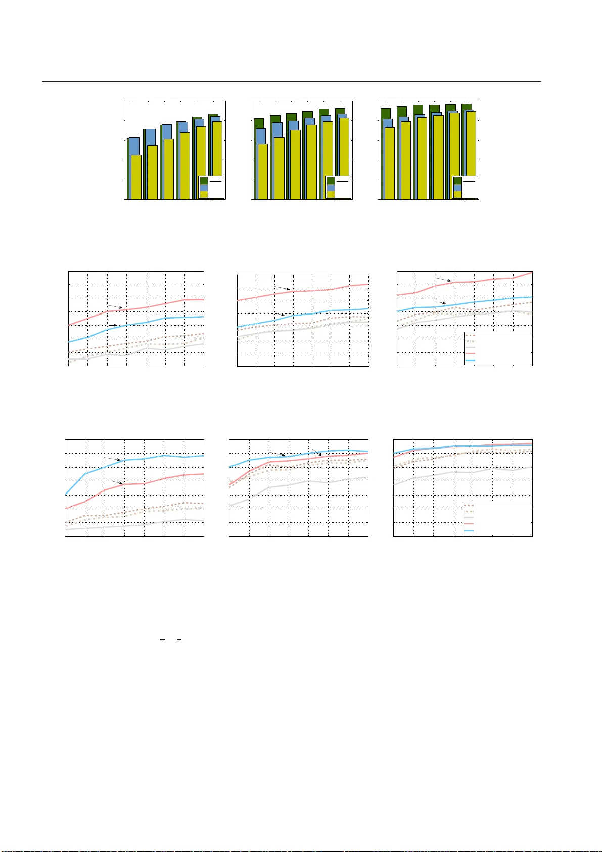
Noname manuscript No. (will be inserted by the editor) Compressi v e Mining: F ast and Optimal Data Mining in the Compressed Domain Michail Vlachos · Nikolao s M. Freri s · Anastasios K yrillidi s Receiv ed: date / Accepte d: date Abstract Real- world data typically contain repeated and periodic pa tterns. This sug gests that they can be e ﬀ ectiv ely represented an d compressed using only a few coe ﬃ cients o f an approp riate basis (e.g., Fourier , W av elets, etc.). However , dis tanc e estimat ion when the data are represented using di ﬀ erent sets of c oe ﬃ cients is still a largely unexplored area. This work studies the optimization problems related to obtaining the tightest lowe r/upper bound on E uclidean distances when each data object is potentiall y compressed using a di ﬀ erent set o f orthonormal co e ﬃ cients. O ur technique leads to tighter dist ance estima tes, which translate s into more accurate search, learning and mining operations di- rectly in the compressed domain. W e formula te the problem of estimati ng lowe r/upper distance bounds as an optimization problem. W e establis h the properties of optimal soluti ons, and le verag e the theoretical analysi s to dev elop a fast algorithm to ob tain an exac t solution to the problem. The sug geste d solution provides the tightest estimation of the L 2 -norm or the correlation. W e s how that typical data- analysis operations, such as k -NN search or k -Means clus tering, can operate more accuratel y using the propo sed compression and distance recon struction technique. W e compare it with many oth er prevale nt compression and recon- struction techniques, including random projections M. Vlachos an d A. K yrillidis IBM-Research Z ¨ urich, S ¨ aumerstrasse 4, CH-8803, R ¨ uschlikon, Switzerland E-mail: { mvl,nas } @zurich.ib m .com N. Freris School of Computer and Communication Sciences, ´ Ecole P oly- technique F ´ ed ´ erale de Lausanne (EPFL ), CH-1015 Lausanne, Switzerland E-mail: nikolaos.freris@epﬂ.ch and PCA -based techniques. W e highlight a surprising resul t , namely that when the data are h ighly sparse in some basis, our technique may ev en outperform PC A -based compression. The c o ntributions of this work are ge neric as our methodology is app licable to an y sequential or high- dimensional da ta as wel l as to any or thogonal data transformation used for the underl ying data co mpres- sion scheme. K eyword s: Data Compression, Compressiv e Sensing, Fourier , W a vel ets, W ater -ﬁlling algorithm, Con vex Optimization 1 Introduction Increasing data sizes are a perennial problem for data analysis. This dictates the need not only for more e ﬃ - cient data-compression schemes, but also for analytic operations that work directl y in the compressed do- main. Co mpression schemes exploit inherent patte rns and structures in the data. In fact, many natural a n d indus trial processes exhibit p atterns and periodicities. P eriodic beha vior is o m n ip r esent; be it in environmen- tal and natural processes [1, 2], in medical and p hys- iological measurements (e .g., EC G data [3 ]), w eblog data [4, 5], o r network measurements [6]. The afore- mentioned are only a few o f the numerous scientiﬁc and indus trial ﬁelds that exhibit repetitions. Examples from some of these areas are shown in F ig. 1 . When data contain an inherent structure, more ef - ﬁcient c o mpression can be performed with m inimal loss in data quality (see Fig. 3 for an example). The bulk of relate d work on compression and distance es- timation used the same sets of co e ﬃ cients for all ob- jects [7, 8, 9, 10]. This simpliﬁed the distance estima- 2 Michail Vlachos et al. Fig. 1: Many scientiﬁc ﬁelds entail periodic data. Ex- amples fr om medical, ind ustrial, web and astronomi- cal measurements. tion in the compressed domain. Howev er , by encod- ing the data using only a few and potentially disj oint sets of high-energy coe ﬃ cients (i.e., coe ﬃ cients of high- est absolut e val ue) in an orthonormal basis, one can achieve better reconstruction performance. Nonethe- less, it was not known how to compute tight distance estimat es using such a representation. Our work ex- actly addres ses this iss ue: given da ta that are com- pressed using disjoint coe ﬃ cient sets of a n orthono r - mal basis (for reasons of higher ﬁdelity), how can dis- tances among the compressed objects be estimated with the highest ﬁdelity ? Here, we provide the tightest possible upper and lowe r bounds on the original distances, based only on the compressed objects. By tightest , we mean that , give n the information av ailable, no better estimate ca n be deriv ed. Distance estimation is fundamental for data mining: the majority of mining and learning tasks are distance-based , includ ing clustering (e.g. k -Means or hierarchical), k -NN classiﬁcation, outlier detection, pattern matching, etc. T his work focuses on the case where the distance is the widely used Eu c lidean dis- tance ( L 2 -norm), but makes no assertions on the un- derl ying transform used to compress the data: As long as the transform is orthonormal, our methodol ogy is applicable. In the experimental section, we use both Fourier and W avelets Decomposition as a data co m- pression technique. Our main contribution s are sum- marized below: - W e formulate the problem of tight distance esti- mation in the compressed domain as two optimization problems for obtaining lower/upper bounds. W e show that both p roblems can be solved simultane ously by solving a single convex optimization program . - W e derive the necessary and su ﬃ cient Karush- K uhn- T ucker (KKT) conditions and study the proper - ties of optimal solu tions. W e use the analysis to devise exact closed-form solution algorithms for the op timal distance bounds. - W e ev aluate our analytical ﬁndings experimen- tally; w e compare the proposed alg orithms with prev a - lent distance estimation schemes, and demonstrate signiﬁcant improveme nts in terms of estimation ac cu- racy . W e further compare the performance of our opti- mal algorithm with that of a numerical scheme based on conv ex optimization, and show that our scheme is at least two orders of ma gnitude faster , while also pro- viding more accurate resul ts. - W e also provide extensive ev aluations with min- ing tasks in the co mpressed domain using our ap- proach and man y other prev alent compression and distance reconstruction schemes used in the literature (random projections, SVD, etc). 2 Related W ork W e brieﬂ y position our work in the co ntext of other similar app r oaches in the area. T he majority of data- compression techniques for sequential da ta use the same s et o f low -energy coe ﬃ cients whether using Fourier [7, 8], W ave lets [9, 10] or Chebyshe v polynomi- als [13] as the orthogonal basis for representation and compression. Using the same set of orthogonal coe ﬃ - cients has several advantag es: a) it is straightf o rward to compare the respectiv e coe ﬃ cients; b) space parti- tioning and indexing structures (such as R -trees) can be directly used on the compressed data; c) there is no need to store also the indices (position) of the basis functions to which the stored co e ﬃ cients correspond. The disadv antage is that both object reconstruction and distance estimation ma y be far from optimal for a given ﬁxed compression ratio. One c an also record side information, such as the energy of the discarded coe ﬃ cients, to better approx- imate the distance between compressed sequences by lev eraging the Ca uchy –S chwartz inequality [14]. This is shown in Figu r e 2a). In [12, 11], the auth ors ad- vocat ed the use of high-energy coe ﬃ cients and side information on the discarded coe ﬃ cients for weblog sequence repositories ; in th at se tting o ne of the se- quences was compressed, whereas the query was un- compressed, i.e., all coe ﬃ cients were avail a ble as illus- trated in Figu r e 2 b). This work examines the most gen- eral an d c hallenging case when both objects are com- pressed. In such case, we record a (gene r ally) di ﬀ erent set o f high-energy coe ﬃ cients and also store aggregate side information, such as the energy of the omitted Compressi ve Mining 3 e e e e e Q X Q X Q X a) b) c) Fig. 2: Comparison with previous work. Distance estimation betwe en a compressed sequence (X) and a query (Q) represented in any complete orthono rmal basis. A compressed sequence is represented by a set of stored coe ﬃ cients (gray) as well as the error e incurred beca use of compression (yell ow). a) Both X,Q are co mpressed by storing the ﬁrst coe ﬃ cients. b) T he highes t -energy coe ﬃ cients are used for X , whereas Q is uncompress ed as in [11, 12]. c) The problem we address: both sequences are co mpressed usi ng the highest -ene rgy coe ﬃ cients; note that in general for each object a di ﬀ erent set of coe ﬃ cients is used. data; this is depicted in Figure 2c ). W e are not aware of an y previous art addressing this problem to derive either optimal or suboptimal bounds on distance esti- mation. The ab ove approaches conside r determining dis- tance estimat ion in the compressed domain. There is also a big b o dy of w ork that considers pr obabilistic distance estimati on via l ow-di mensional embeddings. Several projection technique s for dimensionality re- duction can preserve the geometry o f the p oints [15, 16]. T hese resul ts heavil y depend on the work o f John- son and Lindenstrauss [17], accor ding to which any set of points c an be projected onto a logarithmic (in the cardinality of the data points) dimensional sub- space, while still retaining the relativ e distances be- tween the points, thus preserving an approximation of their nearest neighbors [18, 19 ] or clust ering [20 , 21]. Both random [22] an d deterministic [23] constructions hav e been pr oposed in the literature. This pap er extends and expands the work of [24]. Here we include additional experiments tha t show the performance of our methodology for k -NN-search, and k -Means clustering directly in the compressed do- main. W e also compare our approach with the per - formance of Principal C omponents and Random Pro- jection techniques (both in the tr a ditional and in the compressiv e sensing setting). Final ly , we also conduct experiments using other orthonormal bases (namely , wav elets) to demonstrate the generality of our tech- nique. In the experimental section of th is work, we compare our methodology to both deterministic and probabilistic techniques. 3 Searching Data Using Distance Estimates W e consider a database D B that stores sequences as N -dimensional complex vectors x ( i ) ∈ C N , i = 1 , . . . , V . A search problem that we examine is abstracted as fol- lows: a user is intereste d in ﬁnding the k most ‘simi- lar’ sequences to a give n query sequence q ∈ D B , un- der a certain dist ance metric d ( · , · ) : C N × N → R + . This is an elementary , yet fundamental operation known as k -Nearest -Neighb or ( k -NN)-search. It is a co re func- tion in dat abase-querying, dat a -mining and machine- learning algorithms including classiﬁcation (NN clas- siﬁer), clustering, etc. In this paper , we focus on the case where d ( · , · ) is the Euclide an distance. W e note that other mea- sures, e.g., time-inv ariant matching, c an be formu- lated as Euclidean distance on the periodogram [25]. Correlation can also be expressed as an instance of E uclidean distance on pr operly normalized sequences [26]. Therefore, our approach is applicable on a wide range of distance measures w ith little or no modiﬁca - tion. However , for ease of exposition, we focus on the E uclidean distance as the most used measure in the lit - erature [27]. Search operations can be quite costly , especially for cases when the dimensionality N of data is high: se- quences need to be retrieved fr om the disk for com- parison against the query q . An e ﬀ ectiv e wa y to mit - igate this is to retain a compressed representation of the sequences to be used as an initial pre-ﬁlte ring step. T he set of co mpressed sequences co uld be small enough to keep in-memory , hence enabling a signiﬁ- cant performance speed up. In esse n c e, this is a mul- 4 Michail Vlachos et al. tilevel ﬁltering mechanism. With o nly the c ompressed sequences availab le, we obviousl y cannot infer the ex- act distance betw een the query q and a sequence x ( i ) in the database. Howev er , it is still plausible to obtain lower and upper bounds of the dis tanc e. Using the se bounds, one might request a superset of the k -NN an- swers, w hich will be then veriﬁed using the uncom- pressed se q uences that will need to be fetched and compared with the query , so that the exact distances can be computed. Such ﬁlte ring ideas are used in the majority of the data-mining literature for speeding up search o perations [7 , 8, 28]. 4 Notation Consider an N -dimensional sequence x = [ x 1 x 2 . . . x N ] T ∈ R N . For compress io n purpo ses, x is ﬁrst transformed using a sparsity-i nducing (i.e., compressib le) basis F ( · ) in R N or C N , such that X = F ( x ). W e denote the forward linear map- ping x → X by F , whereas the inv erse linear ma p X → x is denoted by F − 1 , i.e., we say X = F ( x ) and x = F − 1 ( X ). A nonexhaus tive list of invertible linear transformations includes Discrete Fourier T ransform (DFT), Discrete Cosine T ransform, Di screte W av elet T ransform, etc. As a running example for this pa p er , we assume that a sequence is compressed using DFT . In this case, the basis represent sinusoids of di ﬀ erent frequencies, and the pair ( x , X ) satisﬁes X l = 1 √ N N X k =1 x k e i 2 π ( k − 1)( l − 1) / N , l = 1 , . . . , N x k = 1 √ N N X l =1 X l e i 2 π ( k − 1)( l − 1) / N , k = 1 , . . . , N where i is the imaginary unit i 2 = − 1. Given the above, we assume the L 2 -norm as the dis- tance between two sequences x , q , which can easily be translated into distance in the frequency domain be- cause of P arsev al’ s theorem [29]: d ( x , q ) := || x − q || 2 = || X − Q || 2 In the experimental section, we also show app lica- tions of our methodology when wavele ts are used as the signal decomposition transform. 5 Motiva tion The choice of which coe ﬃ cients to use has a direct im- pact o n the data ap proximation quality . It has l o n g been reco gnized that sequence app r oximation is in- deed superior when using high-energy coe ﬃ cients [30, 12]; in fact, using high-energy coe ﬃ cients co rresponds to optimal L 2 compression–as indicated by P arsev al’ s theorem–hence, we also use the term ‘’best coe ﬃ - cients” to refer to the high-energy coe ﬃ cients main- tained during compression; see also Figure 3 for an il- lus trativ e example - However , a barrier still has to be overcome when using optimal l 2 compression: the ef - ﬁciency of solu tion for distance estimation. Consider a sequence represented using its high- energy coe ﬃ cients. Then, the compressed seque nce will be described by a set of C x coe ﬃ cients that hold the largest energy . W e denote the vector describing the positions of those coe ﬃ cients in X as p + x , and the posi- tions of the remaining o nes as p − x (that is, p + x ∪ p − x = { 1 , . . . , N } ). For any sequence X , we store the vector X ( p + x ) in the da tabase, which we denote simply by X + := { X i } i ∈ p + x . W e denote the vector of discarded co- e ﬃ cients by X − := { X i } i ∈ p − x . In addition to the best co- e ﬃ cients of a sequence, we can also record one addi- tional val ue for the energy of the compression err or , e x = || X − || 2 2 , i.e., the sum of squared magnitude s o f the omitted coe ﬃ cients. Then, one needs to solve the following minimiza- tion (maximization) problem for c alcula ting the lowe r (upper) bounds on the distance between two se- quences based on their compressed versions: min (max) X − ∈ C | p − x | , Q − ∈ C | p − q | || X − Q || 2 s.t. | X − l | ≤ min j ∈ p + x | X j | , ∀ l ∈ p − x | Q − l | ≤ min j ∈ p + q | Q j | , ∀ l ∈ p − q X l ∈ p − x | X − l | 2 = e x , X l ∈ p − q | Q − l | 2 = e q (1) The inequality constraints are due to the fact that we use the high-e n ergy components for the compression. Hence, any of the omitted c o mponents must hav e an energy lower than the minimum energy of any kept component. The o ptimization problem presented is a c o mplex- v alued program: we show a single real-v alued convex program that is equi valent to both the minimization and maximization problems. T his program can be solved e ﬃ cientl y w ith numerical methods [31], cf. Sec. 8. 1. Howev er , as we show in the experimental section, eval- uating an instance of this problem is not e ﬃ cient in practice, even for a single pair of sequences. There- fore, although a solution c an be found nu m erically , it is generally costly and not suitable for large min- ing tasks, where one would like to ev aluate thousands Compressi ve Mining 5 a) b) c) Distance = 6.4 Distance = 4.3 Distance = [5.7 ... 7.2] Uncompressed Data Compressed using First Coefficients Compressed using Best Coefficients Goal is to make the lower and upper bounds as tight as possible Fig. 3: Motiv ation for using the high-energy (best) coe ﬃ cients for compression. Using the best 10 co e ﬃ cients (c) resul ts in signiﬁcantly better sequence appro ximation than when using the ﬁrst coe ﬃ cients (b). or millions of lower/upper bounds on co mpressed se- quences. In this paper , we show how to solve this problem anal yt ic all y by exploiti ng the deriv ed optimality con- ditions. In this manner we can solve the problem in a fraction of the time required by numerical meth- ods. W e solve this problem as a ‘double- waterﬁlling’ instance. Vlachos et al. have shown how the opti- mal lower and upper distance bounds betw een a c om- pressed and an uncompressed sequence can be rele- gated to a single wa terﬁlling problem [12]. W e revisit this appr o ach as it will be used as a building block for our solut ion. In addition, we later derive optimality properties for our solution. 6 An Equivalent Conv ex Optimization Problem For ease of notation, we consider the partition P = { P 0 , P 1 , P 2 , P 3 } of { 1 , . . . , N } (see Fig. 4), where we set the following: – P 0 = p + x ∩ p + q are the common known components in two co mpressed sequences X , Q . – P 1 = p − x ∩ p + q are the c omponents unknown for X but known for Q . – P 2 = p + x ∩ p − q are the components known for X but unknown for Q . – P 3 = p − x ∩ p − q are the co mponents unknow n for both sequences. Using the standard notation x ∗ for the conjugate transpos e of a complex vector x , ℜ{ ·} to denote the real part of a complex number , and considering all vectors as co lumn vectors, we have that the squared E uclidean Q X Unknown (Discarded) Coefficient Known (Kept) Coefficient P 0 P 1 P 2 P 3 P 0 P 1 P 2 P 3 P 3 P 3 P 3 P 3 Fig. 4: Visual illustrat ion of sets P 0 , P 1 , P 2 , P 3 betwe en two compressed objects. distance is given by: || x − q || 2 2 = || X − Q || 2 2 = ( X − Q ) ∗ ( X − Q ) = || X || 2 2 + || Q || 2 2 − 2 X ∗ Q = || X || 2 2 + || Q || 2 2 − 4 N X i =1 ℜ{ X i Q i } = || X || 2 2 + || Q || 2 2 − 4( X l ∈ P 0 ℜ{ X l Q l } + X l ∈ P 1 ℜ{ X l Q l } + X l ∈ P 2 ℜ{ X l Q l } + X l ∈ P 3 ℜ{ X l Q l } ) . Note that || X || 2 , || Q || 2 can be inferred by summing the squared magnitudes of the known coe ﬃ cients with the energy of the compression error . Also, the term P l ∈ P 0 ℜ{ X l Q l } is known, whereas the last three sums are unknown. C o nsidering the polar form, i.e., abso- lute v alue | · | and argument arg( · ) X l = | X l | e i arg( X l ) , Q l = | Q l | e i arg( Q l ) , we have that the decision variables are vectors | X l | , arg( X l ) , l ∈ p − x as well as | Q l | , arg( Q l ) , l ∈ p − q . Ob- serve that for x , y ∈ C with | x | , | y | know n, we have that 6 Michail Vlachos et al. −| x || y | ≤ ℜ{ x y } ≤ | x | | y | , w here the upper bound is at - tained when arg( x ) + arg( y ) = 0 and the lower bound when ar g( x ) + arg( y ) = π . Therefore, both problems (1) boil down to the real- v alued optimization problem min − X l ∈ P 1 a l b l − X l ∈ P 2 a l b l − X l ∈ P 3 a l b l (2) s.t. 0 ≤ a l ≤ A , ∀ l ∈ p − x 0 ≤ b l ≤ B , ∀ l ∈ p − q X l ∈ p − x a 2 l ≤ e x X l ∈ p − q b 2 l ≤ e q , where a l , b l represent | X l | , | Q l | , respectiv ely , and A := min j ∈ p + q | X j | , B := min j ∈ p + q | Q j | . Note also that we hav e relaxed the equality constraints to inequalit y con- straints as the objective function of (2) is decreasing in all a i , b i , so the optimum of (2) has to satis fy the re- laxed inequality constraints with equality , becau se of the elementary property that | p − x | A 2 ≥ e x , | p − q | B 2 ≥ e q . Recall that in the ﬁrst sum only { a i } are known and in the second only { b i } , whereas in the third all v ariables are unknown. W e have reduced the o r iginal pr oblem to a single optimization program, which, however , is not convex unless p − x ∩ p − q = ∅ . It is easy to check that the constraint set is conv ex and compact; however , the bilinear func- tion f ( x , y ) := x y is convex in each argument alone, but not jointly . W e consider the re-parametrization of the decision variab les z i = a 2 i for i ∈ p − x , and y i = b 2 i for i ∈ p − q , we set Z := A 2 , Y : = B 2 and get the equiv alent problem: min − X i ∈ P 1 b i √ z i − X i ∈ P 2 a i √ y i − X i ∈ P 3 √ z i √ y i (3) s.t. 0 ≤ z i ≤ Z , ∀ i ∈ p − x 0 ≤ y i ≤ Y , ∀ i ∈ p − q X i ∈ p − x z i ≤ e x X i ∈ p − q y i ≤ e q . The necessary and su ﬃ cient conditions on opti- mality are presented in appendix 12.1. Optimal low er/upper bounds: Let us denote the op- timal valu e of (3) by v opt ≤ 0. Then the optimal lower bound (LB) and upper bound (UB) for the distance es- timation problem under consideration are giv en by LB = q ˆ D + 4 v opt (4) U B = q ˆ D − 4 v opt (5) ˆ D := || X || 2 2 + || Q || 2 2 − 4 X l ∈ P 0 ℜ{ X l Q l } . Remark 1 Interestingl y , the widely used conv ex solver cvx [32] cannot directl y address (3)–the issue is that it fails to recognize convexity of the objective functions. For a numerical solution, we con sider solving a relaxed versi on of the minimization problem (1), where equal- ity constraints are replaced by ≤ inequalities. W e note that this problem is not equiv alent to (1), but still pro- vides a viable lower bound. An upper bound can be obtained by (cf . (4), (5) ): U B = p 2 ˆ D − LB 2 . W e test the tightness of such approa c h in the experi- mental section 10. 7 Exact Solutions In this section, we study alg o rithms for obtaining ex- act solutions for the optimization p roblem (3). By ex- act , we mean that the op timal val ue is obtained in a ﬁnite number o f computations as opposed to when us- ing a numerical scheme for convex o ptimization. In the latter case, an appro ximate solution is obtained by means of an iterat ive scheme which converges with ﬁnite pr ecision. Before addressing the general pro b- lem, we brieﬂy recap a special ca se that was dealt with in [12], where the sequence Q was assumed to be un- compressed. In this ca se, a n exact solution is p r ovided via the waterﬁlling al gorithm, which constitutes a key buil ding block for obtaining exact solutions to the gen- eral p roblem later on. W e then proceed to study the properties of optimal solutions; our theoretical analy - sis gives rise to an exact algorithm, cf. Sec. 8.2. 7.1 W aterﬁlling Algorithm. The c a se that Q is uncompressed is a special instance of our problem with p − q = ∅ , whence also P 2 = P 3 = ∅ . The problem is strictly c onve x, and (A -2d) yiel ds z i =  b i λ + α i  2 ⇔ a i = b i λ + α i (6) In such a case, the strict conv exity guarantees the ex- istence o f a unique solution satisfying the KKT con- ditions as given by the w aterﬁlling algorithm, cf. Fig. Compressi ve Mining 7 5. The algorithm progressivel y increases the unknown coe ﬃ cients a i until sat uration, i.e., until they reach A , in which ca se they are ﬁxed. The set C is the set of no n satura ted coe ﬃ cients at the beginning of each itera- tion, whereas R denotes the “energy reserve,” i.e., the energy tha t can be used to inc rease the non satura ted coe ﬃ cients; v op t denotes the optimal valu e. W aterﬁlling algorithm Inputs: { b i } i ∈ p − x , e x , A Outputs: { a i } i ∈ p − x , λ, { α i } i ∈ p − x , v opt , R 1. Set R = e x , C = p − x 2. while R > 0 and C , ∅ do 3. set λ = q P i ∈ C b 2 i R , a i = b i λ , i ∈ C 4. if for some i ∈ C , a i > A then 5. a i = A, C ← C − { i } 6. else break ; 7. end if 8. R = e x − ( | p − x | − | C | ) A 2 9. end while 10. Set v opt = − P i ∈ p − x a i b i and α i = ( 0 , if a i < A b i A − λ , if a i = A Fig. 5: W aterﬁlling algorithm for optimal distance es- timation between a compressed and an uncompressed sequence As a sh orthand notation, w e write a = wate r ﬁll( b , e x , A ). Note that in this case the prob- lem (2) for P 2 = P 3 = ∅ is c onve x, so the solution can be o btained via the KKT conditions to (2), which are di ﬀ erent fr o m those for the re-parameterized problem (3); this was done in [12]. The analysis and straightforward extensions are summarized in Lemma 1. Lemma 1 (Exact solutio ns) 1. If either p − x = ∅ or p − q = ∅ (i.e., when at least one of the sequences is uncompresse d) we can obtain an ex- act solution to the optimization problem (2 ) via the waterﬁlling algorithm. 2. If P 3 = p − x ∩ p − q = ∅ , i.e., when the two compressed sequences do not have any common unknown coe ﬃ - cients, the problem is decoupled in a , b , and the water - ﬁlling algorithm can be used separately to obtain exact solutions to both unknown vectors. 3. If P 1 = P 2 = ∅ , i.e., when both compressed sequences have the same discarded coe ﬃ cients, the optimal value is simp l y equal to − √ e x √ e q , but there is no un i que so- lution for a , b . Proof The ﬁrst two cases are obvious. For the third o ne, note that it f ollows immediatel y from the Cauch y–Schwartz inequality that − P l ∈ P 3 a l b l ≥ − √ e x √ e q , and in this is case this is also attainable. J ust consider for example, a l = q e x | P 3 | , b l = q e q | P 3 | , which is feasibl e becau se | p − x | A 2 ≥ e x , | p − q | B 2 ≥ e q , as follows by compression with the high-energy c oe ﬃ cients.  W e hav e shown how to obtain exact optimal solu- tions for special cases. T o derive e ﬃ cient al gorithms for the general case, we ﬁrst study and establish some properties of the optimal solution of (3). Theorem 1 (Properties of optimal solutions) Let an augmented optimal solution of (2) be deno ted by ( a opt , b opt ); where a opt := { a opt i } i ∈ p − x ∪ p − q denote s the optimal solution extended to include the known values | X l | l ∈ P 2 , and b opt := { b opt i } i ∈ p − x ∪ p − q denote s the optimal solution ex- tended to include the known values | Q l | l ∈ P 1 . Let us further deﬁne e ′ x = e x − P l ∈ P 1 a 2 l , e ′ q = e q − P l ∈ P 2 b 2 l . W e then have the following: 1. The optimal solution satisﬁes 1 a opt = waterﬁll ( b opt , e x , A ) , (7a) b opt = waterﬁll ( a opt , e q , B ) . (7b) In particular , it follows that a opt i > 0 i ﬀ b opt i > 0 and that { a opt i } , { b opt i } have the same ordering. In addition, min l ∈ P 1 a l ≥ max l ∈ P 3 a l , min l ∈ P 2 b l ≥ max l ∈ P 3 b l . 2. If at optimality it holds that e ′ x e ′ q > 0 there exists a multitude of solutions. One solution ( a , b ) satisﬁes a l = q e ′ x | P 3 | , b l = q e ′ q | P 3 | for all l ∈ P 3 , whence λ = s e ′ q e ′ x µ = s e ′ x e ′ q , (8a) α i = β i = 0 ∀ i ∈ P 3 . (8b) In particular , λµ = 1 and the values e ′ x , e ′ q need to be solutions to the following set of nonlinear equations: X l ∈ P 1 min  b 2 l e ′ x e ′ q , A 2  = e x − e ′ x , (9a) X l ∈ P 2 min  a 2 l e ′ q e ′ x , B 2  = e q − e ′ q . (9b) 3. At optimality , it is not possible to have e ′ x e ′ q = 0 unless e ′ x = e ′ q = 0 . 1 This has a natural interpretation as the Nash equilibrium of a 2-pla yer game [33] in which Player 1 seeks to minimize the objectiv e of (3) with respect to z , and P layer 2 seeks to minimize the same objective with respect to y . 8 Michail Vlachos et al. 4. C onsider the vectors a , b with a l = | X l | , l ∈ P 2 , a l = | X l | , l ∈ P 1 and { a l } l ∈ P 1 = waterﬁll ( { b l } l ∈ P 1 , e x , A ) , (10a) { b l } l ∈ P 2 = waterﬁll ( { a l } l ∈ P 2 , e q , B ) . (10b) If e x ≤ | P 1 | A 2 and e q ≤ | P 2 | B 2 , whence e ′ x = e ′ q = 0 , then by deﬁning a l = b l = 0 for l ∈ P 3 , we obtain a globall y optimal solution ( a , b ) . Proof See appendix 12.2. Remark 2 One may be tempted to think that an op- timal solut io n can be derived by wat erﬁ lling for the coe ﬃ cients o f { a l } l ∈ P 1 , { b l } l ∈ P 2 separatel y , and then allo- cating the remaining energies e ′ x , e ′ q to the coe ﬃ cients in { a l , b l } l ∈ P 3 lev eraging the Ca uchy –Schwartz inequal- ity , the val ue being − p e ′ x q e ′ q . However , the third and fourth pa r ts of Theorem 1 state that this is not optimal unless e ′ x = e ′ q = 0. W e hav e shown that there are two possible cases for an optimal solution of (2): either e ′ x = e ′ q = 0 o r e ′ x , e ′ q > 0. The ﬁrst case is easy to identify by checking whether (10) yields e ′ x = e ′ q = 0. If this is not the case, we are in the latt er case and need to ﬁnd a sol ution to the set of nonlinear equations (9). Consider the mapping T : R 2 + → R 2 + deﬁned by T (( x 1 , x 2 )) := e x − X l ∈ P 1 min  b 2 l x 1 x 2 , A 2  , e q − X l ∈ P 2 min  a 2 l x 2 x 1 , B 2  ! (11) The set of nonlinear equa tions of (9) corresponds to a positive ﬁxed point of T , i.e., ( e ′ x , e ′ q ) = T ( e ′ x , e ′ q ) , e ′ x , e ′ q > 0. Cal culating a ﬁ xed po int of T may at ﬁ rst seem in- volv ed, but it turns out tha t this c a n be acc o mplished exactly and with minimal overhead . The analysis can be found in appendix 12.3, where we pro ve that this problem is no di ﬀ erent from the simplest numerical problem: ﬁnding the roo t of a scalar linear equati on. Remark 3 W e no te that coe ﬃ cients { a l } P 2 , { b l } P 1 are already sorted becaus e of the way we perform compression–by storing high-energy coe ﬃ cients. It is plain to check that all o ther operations can be e ﬃ - ciently implemented, with the averag e c omplexity be- ing lin ear ( Θ ( N ))–hence the term minimum-overhead alg orithm. Remark 4 (Extensions) It is straightforward to see that our appro ach can be applied without modiﬁcation to the case that each p o int is compressed using a di ﬀ erent number of coe ﬃ cients. Additionally , we note here two important extensions of our problem formulation an d optimal algorithm. 1. Consider the case that a data point is a countably in - ﬁnite sequence. For example, we may express a co n- tinuous function via its Fourier series, o r Cheby- shev polynomials expansion. In that case, surpris- ingly enough, our alg orithm c an be applied with- out any alteration. This is becaus e P 0 , P 1 , P 2 are ﬁ - nite sets as deﬁned above, whereas P 3 is now inﬁ- nite. The energy allocation in P 3 can be computed exactly by the same procedure (cf. a p pendix 12.3) and then in P 3 the Ca uchy – Schwartz inequality is again applied 2 . 2. Of particular interest is the case that data are com- pressed using an over -complete basis (also kno wn as frame in the signal-processing literature [29 ]); this ap proach has recently become p o pular in the compressed-s ensing framework [34]. Our method can be extended to handle this important gen- eral case, by storing the compression errors corre- sponding to each given basis, and calculating the lowe r/upper bounds in each one separatel y using our approach. W e leave this direction for future re- search work. 8 Algo rithm for Optimal Distance Estimation In this section, we present an algorithm for obtain- ing the exact optimal upper and lower bounds on the distance between the original sequences, when fully lev eraging all information av ailable give n their co m- pressed counterparts. First , we present a simple nu- merical scheme using a c onve x solver such a s c vx [32] and then use our theoretical ﬁndings to derive an ana- lytical alg orithm which we call ‘double- waterﬁlling’ . 8.1 Convex Programming W e let M := N − | P 0 | , and consider the nontrivial case M > 0. Following the discussion in Sec. 6, we set the 2 M × 1 vector v = ( { a l } l ∈ P 1 ∪ P 2 ∪ P 3 , { b l } l ∈ P 1 ∪ P 2 ∪ P 3 ) and con- sider the foll owing conv ex problem directly amenable to a numerical solu tion via a solv er such as cvx: min P l ∈ P 1 ∪ P 2 ∪ P 3 ( a l − b l ) 2 s.t. a l ≤ A , ∀ l ∈ p − x , b l ≤ B , ∀ l ∈ p − q P l ∈ p − x a 2 l ≤ e x , P l ∈ p − q b 2 l ≤ e q a l = | X l | , ∀ l ∈ P 2 , b l = | Q l | , ∀ l ∈ P 1 2 The pr oof of optimality in this case assumes a ﬁnite subset of P 3 and applies the same conditions of optimality tha t were leverag ed before ; in fact particular selectio n of the subset is not of importance, as long as its cardinality is large enough to ac- commodate t he computed energy a llocation ( e ′ x , e ′ q ). Compressi ve Mining 9 The lowe r bound ( L B ) can be obtained by adding D ′ := P l ∈ P 0 | X l − Q l | 2 to the optimal valu e of (1) and taking the square root; then the upper bound is given by U B = √ 2 D ′ − L B 2 , cf. (4). Double-waterﬁlling algorithm Inputs: { b i } i ∈ P 1 , { a i } i ∈ P 2 , e x , e q , A, B Outputs: { a i , α i } i ∈ p − x , { b i , β i } i ∈ p − q , λ, µ, v opt 1. if p − x ∩ p − q = ∅ then use waterﬁlling algorithm (see Lemma 1 parts 1,2); return ; endif 2. if p − x = p − q then set a l = q e x | P 3 | , b l = q e q | P 3 | , α l = β l = 0 for all l ∈ p − x , v opt = − √ e x √ e q ; return ; endif 3. if e x ≤ | P 1 | A 2 and e q ≤ | P 2 | B 2 then { a l } l ∈ P 1 = waterﬁll ( { b l } l ∈ P 1 , e x , A ) { b l } l ∈ P 2 = waterﬁll ( { a l } l ∈ P 2 , e q , B ) with optimal values v ( a ) opt , v ( b ) opt , respectivel y . 4. Set a l = b l = α l = β l = 0 for a ll l ∈ P 3 , v opt = − v ( a ) opt − v ( b ) opt ; return ; 5. endif 6. Calculate the root ¯ γ as in Remark 5 (a ppendix 12.3) and deﬁne e ′ x , e ′ q as in (A-8). 7. Set { a l } l ∈ P 1 = waterﬁll ( { b l } l ∈ P 1 , e x − e ′ x , A ) { b l } l ∈ P 2 = waterﬁll ( { a l } l ∈ P 2 , e q − e ′ q , B ) with optimal values v ( a ) op t , v ( b ) op t , respectivel y . 8. Set a l = q e ′ x | P 3 | , b l = q e ′ q | P 3 | , α l = β l = 0 , l ∈ P 3 and set v opt = − v ( a ) op t − v ( b ) op t − p e ′ x q e ′ q Fig. 6: Double-wa terﬁlling alg orithm for optimal dis- tance estimation betw een two compressed sequences. 8.2 Double-wa terﬁlling Lev eraging o ur theoretical analysis, we derive a simple e ﬃ cient alg o rithm to obtain an exact solution to the problem of ﬁnding tight lower/upper bound on the distance o f two c o mpressed sequences; we c all this the “double- waterﬁlling algorithm. ” The idea is to obtain an exact solution of (2) based on the results of Theo- rems 1 , 2, and Remark 5; then the lower/upper bounds are given by (4), (5). The algorithm is described in Fig. 6; its pro of o f optimality follows immediatel y from the preceding theoretical analysis. 9 Mining in the compresse d domain In the experimental section, we will demonstrate the performance of o ur methodology when operating di- rectly in the compressed domain for distance-based operations. W e will use two common search an d m in- ing tasks to showcase our m ethodology: ( i ) the k -NN search and ( i i ) the k -Means clustering. P erforming such operations in the compressed domain may re- quire m o diﬁcations in the original alg orithms, because of the uncertainty introduced in the distance estima- tion in the c ompressed domain. W e discuss these mod- iﬁcations in the sections that follow . W e also elaborate on previous state-of -art ap proaches. 9.1 k -NN search in the compressed domain Finding the closest points to a given query p o int is an elementary subroutine to many problems in search, classiﬁcation, and prediction. A brute-f or ce approach via exhaustiv e search on the uncompressed data can incur a prohibitiv e co st [22]. Thus, the capability to work directly in a compresse d domain pro vides a very practical advantag e to any algorithm. In this context , the k -NN problem [35] in the com- pressed domain can be succinctly described as: k -NN Problem: Given a compressed query representation Y Q and k ∈ Z + , ﬁnd the k closest elements X ( i ) ∈ D B w ith respect to the ℓ 2 -norm through their compres sed repr esen- tations Y ( i ) . V arious diverse approaches exist to tackle this problem e ﬃ ciently and robustly; cf., [36 ]. Here, we compare our methodology with two alg o r ithmic ap- proaches of k -NN search in a low -dimensional space: ( i ) Randomized pro jection-based k -NN and ( i i ) PC A - based k -NN. W e describe these appro aches in mor e de- tail. Approximate k -NN using Randomized Projections (RP): One of the most establis hed approac hes for low - dimensional data processing is through the Jo hnson Lindenstrauss (JL) Lemma 3 : Lemma 2 (JL Lemma) Let X = { X (1) , . . . , X ( V ) } be any arbitrary collection of V points i n N dimensions. F or an isometry constant ǫ ∈ (0 , 1) , we can construct with high 3 While JL Lemma applies for any set of points { X (1) , . . . , X ( V ) } in high dimensions, more can be achiev ed if sparse r epresenta- tions of X ( i ) , ∀ i , are kn own to exist a priori . Comp ressive sens- ing (CS) [37] [34] roughly states that a sparse signal, compared with its ambient dimension, can be perfectly reconstructed from far few er samples than dictated by the well-known Nyquist – Shannon theorem. T o this extent , CS theory expl oits the spar - sity to extend the JL Lemma to more general signal classes, n ot restricted to a collection of points X . As a by-product of this extension, the CS version of the JL Lemma constitutes the Re- stricted Isometry Pr operty (RIP). 10 Michail Vlachos et al. Alg orithm 1 RP -based approximate k -NN alg orithm Input: k ∈ Z + , Q , ǫ ∈ (0 , 1) ⊲ k : # of Nearest Neighbors, Q : the tr ansformed uncompressed query X with the tr ansformed elements X ( i ) = F ( x ( i ) ). 1: Select appropriate d = O ( ǫ − 2 log( V )) 2: Construct Φ ∈ R d × N where Φ i j is i.i.d. ∼ N (0 , 1 √ d ) or ∼ Ber {± 1 √ d } or according to (12). 3: for each X ( i ) ∈ X do ( Pre-processing step ) 4: C ompute Y ( i ) = Φ X ( i ) ∈ C d 5: end for 6: Compute Y Q = Φ Q ∈ C d . 7: for each Y ( i ) do ( Real-time execution step ) 8: C ompute k Y Q − Y ( i ) k 2 9: end for 10: Sort and keep the k -closest Y ( i ) ’ s, in the ℓ 2 -norm sense. probability a linear mapping Φ : C N → C d , wh ere d = O ( ǫ − 2 log( V )) , such that (1 − ǫ ) ≤ k Φ ( X ( i ) ) − Φ ( X ( j ) ) k 2 2 k X ( i ) − X ( j ) k 2 2 ≤ (1 + ǫ ) for all X ( i ) , X ( j ) ∈ X . Therefore, instead of working in the ambient space o f N dimensions, we can co nstruct a linear , nearl y i somet - ric map Φ that p rojects the data onto a low er subspace, approximately preserving their relative distances in the E uclidean sense. V ariants of this approach have also been proposed in [38]. As we ar e n o t interest ed in re- covering the entries of X ( i ) in the d -dimensional space, rather than just performing data manipulations in this domain, o n e can control the distortion ǫ so that tasks such as classiﬁcation and clustering can be performed quite accurately w ith low c omputati onal cost. Ho w- eve r , we underline that the J L guarantees are p roba- bilistic and asymptotic, whereas the lower and upper bounds provided by o ur technique cannot be violated. The topic of constructing m atrices Φ that satisfy the J L Lemma with nice properties (e.g., determin- istic c onstruction, low space-complexity for storage, cheap operations using Φ ) is still an op en question, although many ap p roaches have been proposed. Sim- ilar questions also app ear under the tag of locality- sensitive hashing , where sketching matrices “sense ” the signal under consideration. Fortunately , ma ny works hav e proved the existence of random universal m atrix ensembles that sat isfy the JL Lemma with overwhelm- ing p r obabi l ity , thus ignoring the deterministic co n- struction pro perty . 4 Representativ e examples inc lude 4 Recent developme n ts [39] describe deterministic construc- tions of Φ in polynomial time, based on the fact that t he data X is known a priori and ﬁxed. The authors in [39] propose the NuMax alg orithm, a SemiDeﬁnite Programming (SDP) solve r for conv ex nucl ear norm minimization over ℓ ∞ -norm and pos- random Gaussian matrices [40] and random binary (Bernoulli) matrices [41][22]. Ailon and Chazelle [19] propose a fast JL transform for the k -NN problem with faster execution time than its predecessors. Achlioptas [22] proposes a r a n dom ized construction for Φ , both simple and fast, which is suitable for standard SQL - based databas e environments; each entry Φ i j indepen- dently takes o ne of the following v alues: Φ i j =            1 with probability 1 6 , 0 with probability 2 3 , − 1 with probability 1 6 . (12) This has the additional adv antage of p r oducing a sparse transformation matrix Φ which resul ts in co m - putation savings at the data-compressi on step. In our experiments, we shall r efer to the Gaus- sian distributed pro jection matrix a s GRP , the Bernoulli distribute d pro jection matrix as BRP and Achlioptas’ construction ARP . W e omit sophisticated constructions of Φ because o f their incr eased implementa tion com- plexity . Using linear maps Φ ∈ R d × N or Φ ∈ C d × N satis- fying the J L Lemma, one can compress X ( i ) as Y ( i ) = Φ X ( i ) ∈ C d and store only Y ( i ) for further pro cess- ing. Given a compressed representa tion of a query Q , Y Q = Φ Q , o ne c an compute the distances of each Y ( i ) to Y Q and pick the k nearest po ints in the Euclid ean sense. W e provide a pseudo-code description of the above in Algorithm 1. Overall, Alg orithm 1 requires O ( ǫ − 2 V N log( V )) time to preprocess the entries of D B and O ( ǫ − 2 ( V + N ) log( V )) double-si zed space-complexity , in the itive semideﬁnite constraints. Howev er , NuMax has O ( C + N 3 + N 2 C 2 ) time-com plexity per iteration an d overall O ( C 2 ) space- comple xity , where C :=  V 2  ; this renders NuMax prohibiti ve for real-time applications. Such an a pproach is not include d in our experime nts, but we mention it here for completeness. Compressi ve Mining 11 Gaussi an case. In the other two cases, the space com- plexity can be further reduced thanks to the binary representation of Φ . Given a q uery Y Q , Algorithm 1 requires O (max { V , N } · ǫ − 2 log( V )) time-cost. Approximate k -Nearest Neighbors u sing PC A: Instead of projecting onto a randomly chosen low-dime nsional subspace, one can use the most inf ormative sub- spaces to construct a projection matrix, based on X . PC A -based k -NN relies on this pr inc iple: let X : = [ X (1) X (2) . . . X ( V ) ] ∈ C N × n be the data matrix. Given X , one can compute the Singular V alue Decomposi- tion (S V D) X = U Σ V T to identify the d most important subspaces of X , spanned by the d dominant singular vectors in U . I n this case, Φ := U (1 : d , :) works as a low -dimensional linear m ap, biased by the informa- tion contained in X . The main shortcoming of PC A -based k -NN search is the computation of the SVD of X ; generall y , such an operation has cubic complexity in the number of en- tries in X . Moreover , PC A -based pro jection provides no guarantees on the order of distortion in the co m- pressed dom a in: While in most c ases Φ := U (1 : d , :) outperforms RP -based ap proaches with JL guarantees, one can construct test cases where the pairwise po int distances are heavily distorted such that po ints in X might be m a p ped to a single point [22] [39]. Finall y , note that computa tion of the SVD requires the pres- ence of the entire dataset , whereas ap p roaches such as ours operate on a per -object basis. Optimal bounds-based k -NN: Our app roach can easily be adapted to perform k -NN search op erations in the compressed domain. Similar to Algorithm 1, instead o f computing random p rojection matrices, we keep the high-energy co e ﬃ cients for each transformed signal representation X ( i ) (in Fourier , W av elet or other basis) and also r ecord the total discarded energy per object. Following a similar appr oach to compress the input query Q , sa y Y Q , we p erform the op timal bounds p ro- cedure to obtain upper ( u b ) an d lowe r bounds ( ℓ b ) of the distance in the original domain. Therefore, we do not hav e o nly one distance, but can compute three dis- tance proxies based on the upper and lower bounds on the distance: ( i ) W e use the low er bound ℓ b as indicator o f how close the unco mpressed x ( i ) is to the uncompresse d query q . ( i i ) W e use the upper bound u b as indicator of how close the unco mpressed x ( i ) is to the uncompresse d query q . ( i i i ) W e deﬁne the av erage metric ℓ b + u b 2 as indicator of how close the uncompressed x ( i ) is to the uncom- pressed query q . In the experimental section, we evalu ate the per - formance of these three metrics, and show that the last metric based on the averag e distance bound provides the most robust performance. 9.2 k -Means clus tering in the compressed domain Clust ering is a r udimentary mining task for summa- rizing and visualizing large amounts of data. Speciﬁ- cally , the k -clustering problem is deﬁned as follows: k -Clustering Problem: Given a D B containing V com- presse d representations of x ( i ) , ∀ i , and a target number of clusters k , group the compressed data into k clusters in an accurate way through their compressed representa tions. This is an assignment pro blem and is in fact NP - hard [42]. Man y approximations to this p roblem ex- ist , o ne of the most widely- used algorithms being the k -Means cluste r ing algorith [43]. Formally , k -Means clust ering involve s partitioning the V vectors into k clust ers, i.e., into k disjoint subsets G ( t ) (1 ≤ t ≤ k ) with ∪ t G ( t ) = V , such tha t the sum o f intraclass variances V := k X t =1 X x ( i ) ∈ G ( t ) || x ( i ) − C ( t ) || 2 , (13) is minimized, where C ( t ) is the centroid of the k -th clus- ter . There also exist other formalizations for data clu s- tering, based o n either hierarchical clustering (“top- down ” and “bottom-up ” constructions, cf. [44]); ﬂat or centroid-based clustering, or o n spectral-based clus- tering [45 ]. In our subsequent discussions, we focus on the k -Means alg orithm becaus e of its widespread use an d fast runtime. Note also that k -Means is eas- ily amenable for use by our methodol o gy owning to its computa tion o f distances between objects and the derive d centroids. Similar to the k -NN problem case, we consider low -dimensional embedding matrices based on both PC A and randomized constructions [46][15] [20]. W e note that [20] theoretically proves that a speciﬁc ran- dom matrix construction achieves a (2 + ǫ )-optimal k -partition o f the points in the co mpressed domain in O ( V N k ǫ 2 log( N ) ) time. Based on simulated annealing clust ering heuristics, [21] propo ses a n iterativ e pro- cedure where sequential k -means clust ering is per - formed, with increasing projection dimensions d , for better clustering performance. W e r efer the r eader to [20] for a recent discussion of the above a p proaches. Similar , in spirit, to our approach is the work of [42]. There, the authors propose 1-bit Minimu m Mean 12 Michail Vlachos et al. Alg orithm 2 Optimal bounds-based k -Means Input: k ∈ Z + , Y = { Y (1) , . . . , Y ( V ) } ⊲ k : # of clusters, Y ( i ) : Compressed data vectors. 1: Select randomly k centroids C ( t ) , t = 1 , . . . , k , in the comprese d d oma in. ( Initializa tion step ) 2: while Y ( i ) assignment to C ( t ) changes do 3: C ompute optimal lowe r ℓ b and upper u b bounds betwee n each Y ( i ) and C ( t ) , ∀ i , t . 4: For each pair Y ( i ) , C ( t ) calculate a distance metric m i ,t , based on ℓ b and u b . 5: As sign Y ( i ) ’ s to groups G ( t ) such that: G ( t ) = n Y ( i ) | m i ,t ≤ m i ,q , ∀ q , t o . ( Assignment step ) 6: Up date the centroids: C ( t ) = 1 | G ( t ) | P Y ( i ) ∈ G ( t ) Y ( i ) . ( Upd ate step ) 7: end while Square Error (MMSE) quantizers per dimension and clust er , and p r ovide guarantees for clu ster preserva- tion in the compressed domain. Optimal bound s-based k -Means: T o describe how to use our prop osed bounds in a k -clustering task, let G ( t ) , t = 1 , . . . , k , be the k gro ups of a par tition with cen- troids C ( t ) , t = 1 , . . . , k . W e use a modiﬁcation o f Lloyd’ s alg orithm [43] which co nsists of the following steps: Assignment step: Let C ( t ) , t = 1 , . . . , k , be the curr ent centroids. 5 For each compresse d sequence Y ( i ) ∈ D B , we compute the corresponding upper u b and lower ℓ b bounds with respect to every centroid C ( t ) . W e use a distance metric m i ,t , based on u b and ℓ b to decide the assignment of each Y ( i ) to one of the centroids, i.e., G ( t ) = n Y ( i ) | m i ,t ≤ m i ,q , ∀ q , t o . Here, we use m i ,t = u b + ℓ b 2 where u b , ℓ b denote the upper - and lower -bounds between the c o mpressed se- quence Y ( i ) and the centroid C ( t ) ; other distance met - rics can be used depending on the nature and the re- quirements of the problem at hand. Update step: T o update the centroids C ( t ) , we use the av erage rule using the current distribution of points at each cluster , i. e. , C ( t ) = 1 | G ( t ) | X Y ( i ) ∈ G ( t ) Y ( i ) . Distance to new centroids: Recall that each of the com- pressed objects has information only about its high- energy coe ﬃ cients. This set of coe ﬃ cients may be dif - ferent across objects. So, during the above av eraging operation for computing the centroids, we may end up with the new centroids having (potentiall y) all coe ﬃ - cient p o sitions ﬁlled with some energy . Howev er , this 5 For centr oid initialization, one can choose C ( t ) to be ( i ) com- pletel y random points in t he compressed domain; ( i i ) set ran- domly to one of the compressed representations of X ( i ) ∈ DB , or (iii) use the better performing k -Mean s++ initialization alg o- rithm [47, 42]. does not p ose a pro blem for the distance computa tion becaus e the waterﬁlling algorithm ca n compute dis- tance estimat es eve n betw een co mpressed sequences with di ﬀ erent number of coe ﬃ cients. Therefore, we exploit all information av ailable in the co mputed cen- troid, as this does not increase the space complexity of our technique. Alterna tive ly , one co uld keep on ly the top high-energy coe ﬃ cients for the new centroid. Howev er , there is no need to discard this extra infor - mation. The above steps are summarized in Algorithm 2. 10 Experiments Here we conduct a range of experiments to showcase a) the tightnes s of bounds that we calcula te; b) the low runtime to c o mpute those bounds and, c) the compar - ativ e quality of various mining tasks when using the optimal distance estima tes. Our intention in the experimental section is not to focus on a speciﬁc app lication, rather to eval uate dif - ferent methodologies under imple mentation inv ariant settings. This makes the contribution of our work for compression and search mor e generic and fundamen- tal. Datasets: W e use two datasets: ( i ) a weblog time-series datase t and ( i i ) an image dataset consisting o f V ery Large Scale Integration (VLSI) layouts. The weblog dataset consists of approximately 2.2 million da ta v alues, distill ed fr o m past logs of the IBM.com search page. W e created time-series by as- sembling how man y times important keywords were entered at the search page. W e constructed 2 , 150 time- series x ( i ) ∈ R 1024 , corresponding to an equal number of text queries. Each time-series object captures how many times a p articular text query was posed for 1024 consecutiv e days. W e tr an sform the data into a com- pressible form: for each x ( i ) , we compute its Fourier representation X ( i ) ∈ C N . Compressi ve Mining 13 0 1 2 3 [a] First Coeff. [b] Best Coeff. Numerical Optimal bounds 1 . 94 2 . 13 1 . 96 1 . 94 Coefficients = 4 Improvement over [a] = 0.08% Improvement over [b] = 8.98% PC A-based 0 1 2 3 1 . 78 1 . 96 1 . 74 1 . 70 Coefficients = 8 Improvement over [a] = 4.88% Improvement over [b] = 13.38% 0 1 2 3 1 . 68 1 . 67 1 . 44 1 . 39 Coefficients = 16 Improvement over [a] = 17.21% Improvement over [b] = 16.56% 0 1 2 3 1 . 59 1 . 43 1 . 21 1 . 15 Coefficients = 32 Improvement over [a] = 27.32% Improvement over [b] = 19.12% Fig. 7: Comparison of lower and upper bounds for distances for various compression approac hes. Distances are shown normalized with respect to the original distance (black ve r tical line) on the uncompressed data. The red ve rtical line indicat es the bound giv en the PCA -based approach, which uses a ll the dataset to compute the appropriate basis. The second dataset considers images co nsisting of patterns from a da tabase o f VLSI layouts. The dataset is co mprised of ∼ 150 , 000 image s o f size 512x512. T o support translation-inv ariant matching from each im- age, we extract a signature x ( i ) ∈ R 512 . W e describe this process in mo re detail later . Finally , we represent the resul ting signature using the high-energy wav elet co- e ﬃ cients as basis. Detailed information on this appli- cation will be provided late r on. W e take special care to perform a fair comparison of all techniques. For our approach, per compressed object we need to store the following: ( i ) the v alues X ( p + x ) o f each high-energy c oe ﬃ cient , as s double com- plex valu es for the Fourier case (16 bytes each) and s double valu es for the W av elet case (8 bytes each); ( i i ) The positions p + x of the high-energy coe ﬃ cients, as s integer val ues (4 bytes each) and, ( i i i ) the to- tal remaining energy e x of the discarded c oe ﬃ cients, which can be r epresented with one double variable (8 bytes). Overall, our app roach allocate s spac e for r = l 2 s + s 2 + 1 m double valu es for the Fourier case and r = l s + s 4 + 1 2 m double val ues for the W av elet case. W e make sure that a ll approaches use the same space . So , methods that do not require recording of the explicit position of a co e ﬃ cient , in essence, use m o re coe ﬃ - cients than our technique. 10.1 Tightness of bounds and time complexity First , we ill ustrate how tight the bounds computed by both ( i ) deterministic an d ( i i ) probabilistic approaches are. Deterministic approaches : W e consider the following schemes: ( i ) First Coeffs. : this scheme only exploits the ﬁrst s coe ﬃ cients of each Fourier -transformed X ( i ) to suc- cinctly represent the uncompressed data x ( i ) . No further co mputa tion is performed. ( i i ) Best Coeffs. : this scheme only exploits the best s coe ﬃ cients (in ma gnitude sense) of each Fourier - transformed X ( i ) to succinctly represent the un- compressed data x ( i ) . Similarly to ( i ), no further computation is performed. ( i i i ) PCA-based . This technique uses the PC A -based di- mensionality reduction appro ach. No te that this approach requires as input the complete data, and not each object separately . Given the complet e datase t , one can compute its SVD to extract the most dominant subspaces that explain the most v ar iance in the data. T o achiev e dimensionality re- duction, one pro jects the time-series ve c to rs onto the best d -dimensional subspace by multipl ying the dat a points with the set of d dominant left sin- gular vectors. ( i v ) Optimal bounds - Numerical : Here, we use o ﬀ - the-she lf conv ex solvers to nu m erica lly solve problem (1) through second-order optimization schemes. Numerical approaches are not exact and the minimizer lies within a predeﬁned numerical tolerance ǫ . In our experimental setup, we use the well established CVX li brary where (1 ) is solv ed with tolerance ǫ = 10 − 8 . ( v ) Optimal bounds : our approach in which the upper and l ower bounds on the distance are solved using the closed-form waterﬁlling ideas described . 14 Michail Vlachos et al. 0 1 2 3 RP−based Optimal bounds 1 . 30 1 . 94 Coefficients = 4 PC A-based 0 1 2 3 0 . 97 1 . 70 Coefficients = 8 0 1 2 3 0 . 70 1 . 39 Coefficients = 16 0 1 2 3 0 . 49 1 . 15 Coefficients = 32 0 0.5 1 1.5 2 2.5 RP−based Optimal bounds 1 . 08 0 . 82 Coefficients = 4 PC A-based 0 0.5 1 1.5 2 2.5 0 . 86 0 . 77 Coefficients = 8 0 0.5 1 1.5 2 2.5 0 . 65 0 . 72 Coefficients = 16 0 0.5 1 1.5 2 2.5 0 . 47 0 . 63 Coefficients = 32 Fig. 8: Comparison of lower and upper bounds for the RP -based approac h with the PC A -based and optimal bounds appro aches. T op row: dense case; Bottom row: sparse case. All bounds are shown no r malized with respect to the or iginal distance (black vertical line) on the uncompressed data. The av erage PCA -based dist ance over all pairwise distances is denoted by a v ertical r ed line. T o pr ovide a fair comparison, all appro ac hes use the same amount of space per compressed object for all experiments. Probabilistic approaches : Here, any estimation of dis- tances in the original dat a space holds only in prob- ability and in the asymptotic sense. The performance recorded r epresents only an av erage behavior; i.e., we can alwa ys construct adversarial cases where these schemes p erform poorly for a ﬁxed pr ojection matrix. ( i ) RP-based approach : in this case, we randomly genera te GRP / BRP / ARP d -dimensional mappings Φ . As this appro a c h is pro babilistic, we perform 10 3 Monte Carlo iterations to independentl y generate Φ ’ s and implicitl y extract an app r oximate range o f lowe r and upper bounds. Quality of approximation: Using the weblog time-series data, Figure 7 illustra tes the results for various c o m- pression ratios (i.e. number of coe ﬃ cients used). Us- ing the Optimal bounds scheme, we can ac hiev e up to 27% tighter bounds. The Optimal bounds - Numeri- cal approach provides marginally worse resul ts and has a very high computational cost. The comparsion with probabilistic approaches based on Random Projections is shown in Figure 8 (top row). Among the RP-based approaches, the GRP matrices on av erage attain the best approximation o f the or iginal dist ance. W e should highlight , though, that our appro ach computes nontrivial bounds for any pair of compressed sequences , in contrast to RP -based schemes, where the guarantees hold in probability . Furth ermore, to measure the e ﬃ ciency and robust - ness of our approach w hen the da ta is naturally sparse in some basis, i.e., most o f the entries in N -dimensions are zero, we syntheticall y “sparsify” the webl og data: give n each uncompressed sequence X ( i ) , we assume that X ( i ) is perfectly represented by using only 3 s Fourier coe ﬃ cients, where s = { 16 , 32 , 64 } ; i.e., we sub- sample the signal such that only 3 s amo ng N coe ﬃ - cients are nonzero. Then, we keep s coe ﬃ cients. Fig- ure 8 (bottom row) illu strates the performance of our approach as compared to RP -based and PC A -based ap- proaches. As the data under consideration are sparse, e x and e q estimat es are tighter , pr oviding better upper and lower bounds than in the non-sparse c ase (see Fig- ure 8, top row). Running time: The time complexity of each ap- proach under comparison is given in Figure 9. The graph r eports the average running time (in msec) for computing the distance estimate s between one pair of sequences. It is evident that the proposed an- alytical solu tion based o n double- waterﬁlling is at least two orders o f magnitude faster than the numer - ical approach. More importantly , the optimal solu- Compressi ve Mining 15 0 1000 2000 3000 [a] First Coeff. [b] Best Coeff. Numerical RP−Based PCA−based Optimal bounds 1 . 3 msec 1 . 1 msec 1264 . 4 msec 3 . 1 msec 86 . 0 msec 2 . 2 msec 573x Coefficients = 4 0 1000 2000 3000 1 . 3 msec 1 . 2 msec 1279 . 3 msec 3 . 4 msec 85 . 6 msec 2 . 7 msec 469x Coefficients = 8 0 1000 2000 3000 1 . 2 msec 1 . 3 msec 1379 . 2 msec 8 . 8 msec 85 . 8 msec 2 . 3 msec 588x Coefficients = 16 0 1000 2000 3000 1 . 3 msec 1 . 3 msec 1467 . 2 msec 8 . 0 msec 86 . 0 msec 2 . 4 msec 607x Coefficients = 32 Fig. 9: Runtime of v ar io us techniques to co mpute a distance estimate for one pair of objects. tion thro ugh wa terﬁlling is not computationally bur - dening: competing appr o aches require 1-2 msec for computation, whereas the waterﬁlling approach re- quires around 2.5 msec. The small additional time is attribu ted to the fact that the algorithm distributes the currently remaining energy over two to three it - erations, thus incurring only minimal overhead . The numerical solution runs for m ore than 1 sec and is con- sidered impractical for large mining tasks. 10.2 Mining in the compressed domain W e ev aluate the q uality of mining operations when operating directly on the compressed data. W e com- pare with techniques based on PC A and R andom- Projections. Which distance proxy?: While techniques based on PCA and RP provide only a single distance estimate in the compressed doma in, o ur appr o ach pr ovides both a lowe r and an upper bound. Earlier , we explained that one can use one of three potential proxies for the dis- tance: the upper bound u b , the low er bound ℓ b , o r the av erage o f the two. So, ﬁrst , we ev aluate which o f the three metrics provides better distance estimation using a k -NN task on the webl og dataset. Figure 10 shows how mu ch large a percentage of the common k - NN o bjects is returned in the compressed domain, ver - sus those we would have gott en o n the uncompressed data. The experiment is co nducted under increasing number of coe ﬃ cients. O ne can observe that the av er - age of the lower and upper bounds shows overall su- perior performance, and this is the distance proxy we use for the remaining o f the experiments. k -NN performance: As mentioned, we perform com- parisons under fair settings. Each object under our methodology is represented using r = l 2 s + s 2 + 1 m dou- ble variab les using s coe ﬃ cients in the Fourier ba- sis. T o compress each object using RP -based or PCA - based k -NN, we project each sequence on to d dimen- sions such that the r esul ting low- dimensional projec- tion point does not exceed the memory size of r double v alues. The random matrices Φ in the RP -based k -NN are universally near -isometric; i.e., with high probabil- ity , the same Φ matrix serves as a good linear ma p for any input signal, the creation of Φ ’ s is p erformed once o ﬄ ine for each case; thus , we assume that this opera- tion requires O (1) time and space complexity . Figu re 11 displa ys the results, av eraged over 100 queries. Na turally , the PC A -based k -NN ap proach re- turns the best r esul ts becaus e it uses all the data to construct the appr o priate basis on which to project the data. However , it requires the computation of a Singular V alue or Eigen valu e Decomposition, a O ( d N ) (using Krylov power methods [48]) and O ( d 2 N ) time complexity operation in the most favorable and aver - age scenario, r espectively . Sacriﬁcing acc urac y for low c o mplexity , the RP - based ap proaches constitute inexpensive sol utions: constructing ma trix Φ is easy in practice, while binary-b ased matrix ensembles, such as BRP o r ARP matrices, con stitute low s pace-complexity alterna- tive s. Howev er , RP -based schemes are p r obabilistic in nature; they might “ break down ” for a ﬁxed Φ : one can construct adversarial inputs where their p erfor - mance degrades signiﬁcantl y . Our methodol o gy presents a balanced approach with low time and space complexity , while retaining high accuracy of results . Our ap p roach exhibits better performance over all compression rates, compared to the RP -based ap proaches, see in Figure 11. When sparsity is present: Using a similar m ethodology as in the previous section, we test the k -NN p erfor - mance of the v arious approaches when sparsity of the signals is present. W e create sparse representations of the weblog data by subsampling their Fourier repre- sentati on. Figure 12 illustra tes the quality of k -NN us- ing such a spar siﬁed dataset. P er Φ ∈ C d × N matrix in the RP -based and the PCA -based k -NN, we pr oject 16 Michail Vlachos et al. 10 20 30 40 50 60 0 20 40 60 80 100 k Preserved k - NNs (%) Coe ﬃ cient s = 16 u b + ℓ b 2 u b ℓ b 10 20 30 40 50 60 0 20 40 60 80 100 k Preserved k - NNs (%) Coe ﬃ cient s = 128 u b + ℓ b 2 u b ℓ b 10 20 30 40 50 60 0 20 40 60 80 100 k Preserved k - NNs (%) Coe ﬃ cient s = 384 u b + ℓ b 2 u b ℓ b Fig. 10: Comparison of distance-estimat io n metrics for the k -NN task using the weblog data. The bars depict mean val ues of 100 Monte Car lo iterations. 10 20 30 40 50 60 70 80 30 40 50 60 70 80 90 100 k Preserve d k - NNs (%) Coe ﬃ cient s = 16 Our a ppro ach PC A-ba sed 10 20 30 40 50 60 70 80 30 40 50 60 70 80 90 100 k Preserve d k -NNs (%) Coe ﬃ cient s = 32 Our ap proa ch PC A-ba sed 10 20 30 40 50 60 70 80 30 40 50 60 70 80 90 100 k Preserve d k - NNs (%) Coe ﬃ cient s = 64 GRP BRP ARP PCA Optimal b ounds Our a ppro ach PC A-ba sed Fig. 11: Comparison of the algorithms under c o nsideration for the k -NN task, where X ( i ) / x ( i ) is o r iginally dense. The curves depict mean val ues of 100 Monte Car lo iterat io ns. 10 20 30 40 50 60 70 80 20 30 40 50 60 70 80 90 k Preserve d k -NNs (%) Coe ﬃ cient s = 16 PC A-ba sed Our a ppro ach 10 20 30 40 50 60 70 80 20 30 40 50 60 70 80 90 k Preserve d k -NNs (%) Coe ﬃ cient s = 32 PC A-ba sed Our a ppro ach 10 20 30 40 50 60 70 80 20 30 40 50 60 70 80 90 k Preserve d k -NNs (%) Coe ﬃ cient s = 64 GRP BRP ARP PCA Optimal b oun ds Fig. 12: Comparison o f the alg o rithms under c o nsideration for the k -NN task, where each webl o g sequence is sparsiﬁed to contain only 3 s coe ﬃ cients, w here s = { 16 , 32 , 64 } . The curve s depict mean val ues of 100 Monte Carl o iterations. each weblog signal onto a d -dimensional (complex v al- ued) space, where d = ⌈ s + s 4 + 1 2 ⌉ . Figu re 12 reveals a notable behavior of our model: When X ( i ) is sparse, each X ( i ) can be more accuratel y represented (and thus compressed) using fewer coe ﬃ - cients. Thus, on av erage, the energy discarded e x is also limited. Alterna tively put, the constraint P l ∈ p − x | X ( i ) l | 2 ≤ e x in (1) highly restrict s the candidate space that the un- compresse d signal x ( i ) resides in , r esul ting in tighter up- per and low er bounds. On the other hand, when com- pressing dense X ( i ) ’ s into s coe ﬃ cients, w here s ≪ N , e x provides a large amount of uncertainty as to the reconstruction of x ( i ) . This leads to less tight distance bounds and thus degraded performance. In summary , under high da ta-sparsity , our ap- proach provides superior results in revealing the true k -NNs in the uncompressed domain. Our app roach eve n outperforms PC A -based techniques, and more importantly , our method has a very low computational cost. Clustering quality: W e assess the quality of k -Means clust ering operations in the compressed domain using Compressi ve Mining 17 the original webl og dat aset. The quality is ev aluated in terms of how similar the clusters are before and af - ter c ompression when k -Means is initialized using the same seed points. So, we use the same centroid points C ( t ) as in the uncompressed domain and then co m- press each C ( t ) accordingly , using the dimensionality reduction strategy dictated by each algorithm. The quality resul ts of the algorithms under c om- parison are depicted in Figure 13. W e perform k - Means for di ﬀ erent compression ratios (coe ﬃ cients) and for di ﬀ erent numbers of clus ters k . T he PCA - based ap proach returns the best performance, but in- troduces very large c omputati onal demands due to SVD/Eigen valu e computation. The p erformanc e o f our methodol o gy lies in-betwee n PC A a n d R andom- Projection techniques. 10.3 Using a di ﬀ erent basis (wa velets) In the pr eceding sections we used Fourier decomposi- tion a s our compression method. Now we use wav elets [49] to show the generality of our technique. W e also use a very large image dataset co nsisting of VLSI pat - terns obtained by the semiconductor department of our organ ization. In the remainder of this subsection we ( i ) p rovide an overview of the tasks and challenges related to the speciﬁc dom a in and, ( i i ) show the performance of k - NN search operations on this large real-wor ld dataset. P attern detection on VLSIs: During the production of VLSI circuits (i.e., CPUs), a series of parameters and design protocols shoul d be satisﬁed to ensure that the resul ting product w ill not fail during the manufac- turing process. For example, there are v arious layouts conﬁgurations , that have been known to cause short - circuits and jeopardize the reliability of a circuit. The absence of such artifacts guarantees that the circuit will connect as desired and ensures a margin of safety . A nonexhaustiv e list o f parameters includes the width of metal wires, minimum distances between two adja- cent objects, etc. W e refer the reader to Figu r e 14 for some illu strations. Design-rule checking (DRC) is the process of checking the sat isﬁability of these rules. As a result of a testing process, a collection of VLSI designs ar e annotated as faulty or functional. Now , each newly -pro duced circuit layout is classiﬁed as potentially -faul ty based on its similarity to an al- ready annotated circuit. Novel desi gns, never seen be- fore, need to be tested f urther . Therefore, the testing process can be relegated to a k -NN search operation. The whole process needs to be both expedient and accurate, so that design and production are properly streamlined. Based on an alg ebra of polygons [51 ], a strategy to compare di ﬀ erent layouts is by projecting their binary , 2D description o nto one of the axes. This genera tes a descriptiv e vector per layout as the summary scanned from left to right or from top to bottom, see Figu re 14. Thus, each VLSI layout can be app roximately (but not uniquel y) represented by a signature as the sum along rows or columns. Note that not only this format can be stored and processed more e ﬃ ciently , but it also allows a translation-inv ariant matching of the shape. One can use both row- wise and co lumn-wise signa- tures, but for the purposes of our experiments, we only use the column- wise signature. VLSI datase t: Our original dataset consists of ap prox- imatel y 150 , 000 binary VLSI images, each o f dimen- sion 512x512. W e convert each image into a signature ℓ ( i ) ∈ R 512 , ∀ i , as the column-su m of each image. Fig- ure 15 depicts an instance of a layout image and its resul ting signature. Afterwards, we compress each signa ture using the wav elet transformat ion [49]: L ( i ) = WVL  ℓ ( i )  ∈ R 512 , ∀ i , where WVL ( · ) represents the wa velet linear op erator with minimum scale J min = 2. Observe in the r ight part of Figure 15 that L ( i ) is highly compressible: the energies of wa velet components deca y rap idly to zero according to a power -law decay model of the form:       L ( i )  j      ≤ R · j 1 / p , R > 0 , ∀ j , (14) for som e r and p . This suggest s that each signature is highl y compressible with minimal loss in acc urac y . k -NN results on VLSI layouts: W e ev aluate the q uality of the results of k -NN operations in the compressed domain as c ompared to the k -NN resul ts when o per - ating on the uncompressed image data. W e limit our ev aluation to c omparing our methodology to R andom- Projection techniques, since only these approaches are scalable for large datasets. Figu re 16 illust rates the performanc e of the fol- lowing appr o aches: ( i ) RP -based k -NN for three dif - ferent r andom matrix ensembles (Gaus sian, Bernoulli and Achlioptas’ based) and ( i i ) our Optimal Bounds approach. W e observe that our method can improve the relative e ﬃ ciency of matching by up to 20%, com- pared with the best ra n dom -p r ojection approach. Fi- nally , F igure 17 p rovides some r epresentati ve exam- ples of the k = 5 nearest neighbors for four randomly selected queries. Using the la yo ut signature derived, 18 Michail Vlachos et al. 0 50 100 150 200 250 0 20 40 60 80 100 Coe ﬃ cient s Preserve d Cluster Assignments (%) Clusters = 5 Our a ppro ach PC A-ba sed 0 50 100 150 200 250 0 20 40 60 80 100 Coe ﬃ cient s Preserve d Cluster Assignments (%) Clusters = 10 Our a ppro ach PC A-ba sed 0 50 100 150 200 250 0 20 40 60 80 100 Coe ﬃ cient s Preserve d Cluster Assignments (%) Clusters = 20 GRP BRP ARP PCA Optimal b oun ds Our a ppro ach PC A-ba sed Fig. 13: Assessing the q uality of k -Means cluste r ing in the compressed domain. Fig. 14: Left: Subset of design par a m eters to be satisﬁed during the manufactu r ing [50]. Width and spacing are single la yer rules, where the VLSI layout is seen as a 2D object. A width rule speciﬁes the minimum width of objects; a spacing rule speciﬁes the minimum distance betw een two a djacent objects. Enclosing deals with mul ti-layer rules is not c o nsidered here. R ight: In the left -to-right scanning strategy , moving a vertical scan line horizontally across the layout , we can ma intain the sum of p o lygons observed. As the scan line adv a n c es, new objects are added and old ones are removed. n n 100 200 300 400 500 100 200 300 400 500 0 100 200 300 400 500 0 100 200 300 400 500 n Co l u m n su m 64 192 320 448 −2000 −1000 0 1000 2000 3000 n Am pl i tu de Fig. 15: Lef t panel: Original 2D layout example. White areas indicat e the presence of objects, e.g., metal w ires. Center panel: Co lumn-su m representation o f po lygons in R 512 . Right panel: Amplitude of wave let transforma- tion on the column-sum r epr esentat io n: the majority o f the energy can be captured in only a few coe ﬃ cients. Compressi ve Mining 19 0 100 200 300 400 500 60 70 80 90 100 k Preserve d k -NNs (%) Coe ﬃ cient s = 16 Our ap proa ch 0 100 200 300 400 500 60 70 80 90 100 k Preserve d k -NNs (%) Coe ﬃ cient s = 32 Our ap proa ch 0 100 200 300 400 500 60 70 80 90 100 k Preserve d k -NNs (%) Coe ﬃ cient s = 64 GRP BRP ARP Optimal b ounds Our ap proa ch Fig. 16: k -NN preserv ation performanc e as function of k . Here, the cardinality of D B r is | V | = 149 , 245 and the byte size of each sequence is d bytes. 4 -NN 5 -NN 1 -NN 2 -NN 3 -NN 3 -NN 4 -NN 5 -NN Que ry 1 -NN 2- N N 4 -NN 5 -NN Que ry 1 -NN 2- N N 3- N N 4 -NN 5 -NN Que ry 1 -NN 2- N N 3- N N Que ry Fig. 17: Illus trativ e examples of the Optimal Bounds approach performance for the k -NN pro blem. The leftmost images are the query images, and on the right we depict the k = 5 nearest neighbors as computed in the com- pressed domain. O bserve that owing to the signature extracted f rom each image, we can also detect translation- inv ariant matche s. we can dis cover ve ry ﬂexible translation-in variant matches. Clustering quality on VLSI layouts: W e assess the qual- ity of k -Means clust ering operations in the compressed domain. As before, the quality is ev aluate d as to how similar the cluste rs are before and af ter compres- sion when k -Means is initialized using the same seed points. So, we use the same c entro id points C ( t ) as in the uncompressed domain and then compress each C ( t ) accordingly , using the dimensionality r eduction strategy dictated by each algorithm. Again, we con- sider the k -Means algorithm as our baseline proc e- dure. 20 Michail Vlachos et al. 0 20 40 60 80 100 120 20 40 60 80 100 Coe ﬃ cient s Preserve d Cluster Assignm ent s (%) Clusters = 5 Our a ppro ach 0 20 40 60 80 100 120 20 40 60 80 100 Coe ﬃ cient s Preserve d Cluster Assignm ent s (%) Clusters = 10 Our a ppro ach 0 20 40 60 80 100 120 20 40 60 80 100 Coe ﬃ cient s Preserve d Cluster Assignments (%) Clusters = 20 GRP BRP ARP Optimal b oun ds Our a ppro ach Fig. 18: Clustering preserva tion performance as function of the number of c oe ﬃ cients s . R P -based approaches project onto a d -dimensional subspace, where d = ⌈ 2 s + s 2 + 1 ⌉ . Here, the cardinality of the dataset is | V | = 50 , 000 and the byte size of each sequence is d bytes. Figu re 18 depicts the results for three clustering lev els k : 5, 10 and, 20 clu sters. W e perform k -Means for di ﬀ erent compression ratios (coe ﬃ cients) in the range s = { 4 , 8 , 16 , 32 , 64 , 128 } . W e ev aluate how strong the distortion in cluste r ing assignment is when oper - ating in the compressed domain compared witg the clust ering on the original data. For all cases, our ap- proach provides clus ter output tha t aligns bette r with the original clustering. For this dataset we observ e a consistent 5 − 10% improv ement in the cluster quality returned. These trends are captured in Fi g. 18. In summary , the abov e experiments hav e provided strong evidence that our methodology can o ﬀ er bet - ter mining quality in the compressed domain than random p r ojection techniques , both in the traditional and in the co mpressed-sensing sense (i.e., high data- sparsity). Finally , because our appro ach is also very fast to compute (e.g. co mpared with PC A), we believ e that it will provide an important building block for transitioning many mining operations into the co m - pressed data spac e. 10.4 Indexing In this ﬁnal section we discuss how the prop o sed rep- resentati on and distance estimation scheme can be lev eraged for indexing. The preceding experiments hav e sugg ested that: – The pro posed r epresentati on can exploit patt erns in the dataset to achieve high co mpression. This will r esult in a smaller index size. – The distance estimation (lower -, upper -bounds) are tighter than competitiv e techniques . This eventu- ally leads to better pruning power during search. Note that using the presented variabl e coe ﬃ cient representation traditional space-partitioning indices, such as R -trees o r KD-trees, cannot be used. This is be- cause such techniques assume that each object is r ep- resented by the same set o f coe ﬃ cients, whereas our technique may use: a) potentiall y disjoint sets of coef - ﬁcients per object and/or b) variable number o f coe ﬃ - cients per o bject. Our representati on can be indexed using met - ric trees which create a hierarchical organization of the compressed objects based on their respective dis- tances. In pr evious work we hav e shown how V P -trees (a variant o f metric trees) can be used to index repre- sentati ons tha t use variab le sets of coe ﬃ cients [11]. A VP -tree is constructed by recursiv ely partitioning the objects according to their distance to some selected objects. These objects are called vantage points (VP), and are selected in such a wa y so that they provide a good separation of the currently examined subset o f the dataset . Search and pr uning of the tree is facili- tated using triangle inequality . Q ueries are compared with the vantage point at the current tree level, and search is directed towards the most promising part of the tree. P arts of the tree that ar e pro v ably out - side the search scope (invoking triangle inequality) are pruned from examination. For additional details the interested reader can consult [11]. Indexing setup: W e use three instances from the V LSI datase t: with 10K, 20K and 50K objects, compressed using wavele t coe ﬃ cients. Objects are represented in the compressed domain using s = 4, s = 8 and s = 16 coe ﬃ cients per object. W e use 100 o bjects as queries, which are not the same as the indexed objects . T o construct and search the tree on the compressed objects we use the presented double-w aterﬁlling al- gorithm. The algorithm is used to compute distances both between o bjects for the tree construction phase, as well as for computing distances between the query posed and the tree ’ s v antage p oints. There ar e two Compressi ve Mining 21 0 20 40 60 80 100 10NN 5NN 1NN 92.3 92.2 88.8 92.9 92.4 90.2 92.9 92.8 91.2 Data Pruning (%) VLSI 10K 4 coeffs 8 coeffs 16 coeffs 0 20 40 60 80 100 10NN 5NN 1NN 92.9 92 90.6 94.2 93 91.2 94.6 94 92.2 Data Pruning (%) VLSI 20K 4 coeffs 8 coeffs 16 coeffs 0 20 40 60 80 100 10NN 5NN 1NN 95.4 93.8 93.1 95.9 94.6 93.9 96.4 95.7 94.6 Data Pruning (%) VLSI 50K 4 coeffs 8 coeffs 16 coeffs 0 20 40 60 80 100 10NN 5NN 1NN 95.3 93.8 91.5 96.4 93.9 91.8 96.6 94 92.2 Data Pruning (%) VLSI 10K 4 coeffs 8 coeffs 16 coeffs 0 20 40 60 80 100 10NN 5NN 1NN 94.9 93.8 92.9 96 95.4 94.7 96.6 96 95.7 Data Pruning (%) VLSI 20K 4 coeffs 8 coeffs 16 coeffs 0 20 40 60 80 100 10NN 5NN 1NN 97 96.7 96.2 97.3 96.9 96.8 97.9 97.6 97.5 Data Pruning (%) VLSI 50K 4 coeffs 8 coeffs 16 coeffs Fig. 19: Pruning po wer of a VP -tree index when using the proposed object representa tion and double-wa terﬁlling distance estimation. T op row: conserva tive pruning. Bottom row: aggressiv e pruning. search and pruning strategies one can follow: a con- servative and an aggressive pruning strategy . For the conserv ative strategy both lower and upper bounds (double- waterﬁlling process) from the query to each v antage po int are used to naviga te the tree and prune nodes. For the aggressive pruning strate gy only the av - erage distance ( u l + l b ) / 2 is used as the distance proxy betwe en the query and a vantag e point. The aggres- sive strategy achieves gr eater pruning but this resul ts in slightl y lower pr ecision compared to the co nserv a- tive strateg y . Howeve r the precision of the aggress ive search is still kept at very levels, ra n ging from 75 − 90% across all experiments. In Fi gure 19 we repor t the pruning power achieved with the use of the index for both conserva tive and aggressiv e pruning strategi es. Pruning power is ev al- uated as the number of leave s acc essed over the total number of o bjects in the index. W e calculate the prun- ing power when running 1NN, 5NN and 10NN (Near - est Neighbor) search on the query objects. One can see that with the use of indexing we can refrain from ex- amining a v ery big p art of the dat aset , w ith the prun- ing co nsistentl y exceeding 90%. It is important to no te that the pr uning power gro ws for increasing dataset sizes. 11 Conclusion W e have examined how to compute optimally-tig ht distance bounds on compressed data representations under any or thonormal transform. W e have demon- strated that our methodology can retrieve more rele- v ant match es than competing ap p roaches during min- ing operations on the compressed data. A p a r ticularl y interesting result is that for data w ith very high re- dundancy/sparsity (see, for example, magnetic r eso- nance imaging [37 ]), our app roach may even provide better search performance than compressed sensing approaches, which hav e been designed to speciﬁcally tackle the sparsity issue. In such scenarios, our method may even outperform PCA -based techniques, owing to its capability to use di ﬀ erent sets of high-energy coef - ﬁcients per object. As future work, we intend to continue to inv esti- gate the merits of our methodology under a broader v ar iety of distance-based operations such as anomaly detection and density -based clustering. Acknowledgements: The research leading t o these r esults has receiv ed funding from the Europe a n Research Council under the Europe an Union ’ s Seventh Framework Programme (FP7/2007-201 3) / ERC grant agreement no. 259569 . 22 Michail Vlachos et al. References 1. A. Souza an d J. P in eda, “Tidal mixing modulation of sea surface temperature and diatom abundan ce in Southern California,” in Continental Shelf Research, 21(6-7) , pp. 651– 666, 2001. 2. P . Noble and M. Wheatland, “Modeling the sunspot number distribution with a fokker -planck equation,” The Astrophys- ical Journal , vol. 732, no. 1, p. 5, 2011. 3. G. Ba echler , N. Freris, R. Quick, and R. Crochiere, “Finite rate of innovation based modeling an d compressio n of ECG signals,” in Proceedings of the International Confer ence on Acoustics, Speech and Signal P rocessing (ICA SSP) , pp. 1252– 1256, 2013. 4. S. Chien an d N. Immorli ca, “Semantic similarity betw een search engine queries using t emporal correlation,” in Pro- ceedings of W orld Wide W eb conference (WWW 2005) , 2005 . 5. B. Liu, R. J ones, and K. L . Klinkner , “Measuring the mean- ing in time series clustering of text search q ueries,” in Pro- ceedings of the AC M International Confer ence on Information and Knowledge Management , pp. 836–837, A CM, 2006. 6. E. Nygren, R. K. Sitaraman, and J. W ein, “Networke d sys- tems research at akamai,” A CM SIGOPS Operating Sys tems Review , vol. 44, no. 3, pp. 1–1, 2010. 7. R. Ag rawal, C. F aloutsos, and A. Swami, “E ﬃ cient similar - ity search in sequence databases,” in Proceedings of the In- ternational Confer en ce of F oundations of Data Organization (F ODO) , pp. 69–84, 1993. 8. D. Raﬁei and A. M endelzon, “E ﬃ cient retrieval of sim- ilar time sequences using dft,” in Proceedings of the In- ternational Confer en ce of F oundations of Data Organization (F ODO) , pp. 1-15, 1998. 9. F .-P . Chan, A.-C. Fu, and C. Y u, “Haar wave lets fo r e ﬃ - cient similarity search of time-series: with and without time warping,” IEEE T ransactions on Knowledge and Data Engi- neering , vol. 15, n o. 3, pp. 686–70 5, 2003 . 10. V . Eruhimov , V . Martyanov , P . Raulefs, and E. T uv , “Com- bining unsupervised an d supervised approaches to feature selection for multiv ar iate signal compression,” in Intelli- gent Data Engineering and Automated Learning , pp. 480–487, 2006. 11. M. Vlachos, S. Kozat, and P . Y u, “Optimal distance bounds for f a st search on compressed time-series query logs ,” in A CM T ransactio ns on the We b, 4(2) , pp. 6:1–6:2 8, 2010. 12. M. V lachos, S. Kozat, and P . Y u, “Optimal Distance Boun ds on Time-Series Data,” in Proceedings of SIAM Data Mining (SD M) , pp. 109–120, 2009 . 13. Y . Cai and R. Ng, “Indexing spatio-temporal trajectories with chebyshev polynomials,” in Proceedings of the A CM SIGMOD International C onference on Management of Data , pp. 599–610, A CM, 2004. 14. C. W ang and X. S. W an g, “Multilev el ﬁltering for high di- mensional nearest neighbor search,” in Proceedings of A CM SIGMOD W orkshop on Res earch Issu es in Data Mining and Knowledge , Citeseer , 2000. 15. S. Dasgupta, “Experiments with random projection,” in Proceedings of Conference on Uncertainty in Artiﬁcial Intel- ligence , pp. 143–151, Morgan Kaufmann Publishers Inc., 2000. 16. R. Calderbank, S. Jaf arpour , and R. Schapire, “Compressed learning: Universal sparse dimensionality reduction and learning in t he m easurement domain,” T echnical Report (Princeton University) , 2009. 17. W . B. Johnson and J. Lindenstrauss, “Extensions of Lipschitz mappings into a Hilbert space,” Contemporary Mathematics , vol. 26, pp. 189– 206, 1984 . 18. P . Indyk and A. Naor , “Nearest -neighbor -preserving em- beddings,” A C M T ransactio ns on A lgorithms (T A LG) , vol. 3, no. 3, p. 31, 2007. 19. N. Ailon and B. Chazelle, “ Approximate nearest neighbors and the fast Johnson-Lindenstrauss tran sform,” in Proceed- ings of A CM sy mposium on T heory of Computing , pp. 557– 563, A CM, 2006. 20. C. Boutsidis, A. Zouzias, an d P . Drineas, “Ran dom Projec- tions for k -means Clustering,” in Advances in Neural Infor - mation Processing Systems , pp. 298–306, 2010 . 21. ˆ A. Ca r doso and A. Wichert, “Iterative ran dom projections for high-dimensional data clustering,” Pattern Recognition Letters 33(13) , pp. 1749–17 55, 2012. 22. D. Achlioptas, “Database-friendl y rand om projections,” in Proceedings of A CM Symposium on Principles of Database Sys- tems (PODS) , pp. 274– 281, 2001. 23. E. Bingham and H. M a nnila, “Random projection in dimen- sionality reduction: applications to imag e and text data,” in Proceedings of AC M SIGKDD International Conference on Knowledge Discovery and Data Mining (KDD) , pp. 245–250, A CM, 2001. 24. N. M. Freris, M. Vlachos, and S. S. Kozat, “Optimal distance estimation between compressed data series.,” in Proceedings of SIAM Data Mining (SD M) , pp. 343–354 , 2012. 25. M. Vlachos, P . Y u, and V . Castelli, “On periodicity detection and str uctural periodic similarity ,” in Proceedings of SIAM Data Mining (SD M) , pp. 449–460, 2005 . 26. A. M ueen, S. Nath, and J. Liu, “Fast approximate correla- tion for massive t ime-series data,” in Proceedings of the A CM SIGMOD International Confer ence on Management of Data , pp. 171–182, A CM, 2010. 27. E. Keogh an d S. K asetty , “On the Need for Time Series Data Mining Benchmarks: A Survey and Empirical Demonstra- tion,” in Proceedings of A C M SIGKDD International Confer - ence on Knowledge Discovery and Data Mining (KDD) , 2002. 28. A. M ueen, E. J. Keogh, an d N. B. Shamlo, “Finding Time Series Motifs in Disk -Resident Data,” in Proceedings of the IEEE International Confere nce on Data Mining (ICD M) , pp. 367–376, 2009. 29. A. V . Oppenheim, R. W . Schafer , J. R. Buck, et al. , Discrete- time signal processing , vol. 5. P rentice Hall Upper Saddle River , 1999. 30. E. Keogh, K . Chakrabarti, S. Mehrotra, and M. P azzani, “Locally Adaptive Dimensionality Reduction for Index- ing La rge Time Series Databases,” in Proceedings of A C M SIGMOD W orkshop on Research Issues in Data Mining and Knowledge , pp. 151–162, 2001 . 31. S. Boyd and L . V andenberghe, Convex Op tim ization . Cam- bridge University Press, 1st ed., 2004. 32. M. Grant and S. Boyd, “Gra ph Implementations for Nons- mooth Convex Programs,” Recent Advances in Learning and Contro l, Springer , pp. 95–11 0, 2008 . 33. T . Basar and G. J. Olsder , Dynamic Noncooperative Game The- ory . Academic Press, 2nd ed., 1995. 34. D. L . Donoho, “Compressed sensing,” IEEE T ransactio ns on Information Theory , vol. 52, no. 4, pp. 1289–130 6, 2006. 35. T . Cover and P . Hart, “Nearest neighbo r pattern classiﬁca- tion,” IEEE T ransactions on Information Theory , vol. 13, no. 1, pp. 21–27, 1967. 36. P . W . J ones, A. Osipov , an d V . Rokhlin, “Randomized ap- proximate nearest neighbors algorithm,” in Proceedings of National Academy of Sciences , vol. 108, no. 38, pp. 156 79– 15686 , 2011. 37. E. J. Candes, J. K . Romberg, an d T . T ao, “Stable signal recov- ery from incomp lete and inaccurate measurements,” Com- munications on Pure and A pplied Mathematics , vol. 59, no. 8, pp. 1207–122 3, 2006. Compressi ve Mining 23 38. E. Kushile vitz, R. Ostrovsky , and Y . Rabani, “E ﬃ cient search for approximate nearest neighbor in high dimensional spaces,” SIAM Journal on Computing , vol. 30, n o. 2, pp. 457– 474, 2000. 39. C. Hegde, A. Sankaranar ayanan, W . Yin, and R. Baraniuk, “A convex approach fo r learning near -isometric linear em- beddings,” preprint, August , 2012. 40. S. Dasgupta, “Learning mixtures of Gaussians,” in Pro- ceedings of Symposium on F oundations of C omputer Science (F OCS) , pp. 634– 644, IEEE, 1999. 41. R. I. Ar riaga and S. V empala, “An alg orithmic theory of learning: Robust concepts an d random projection,” in Pro- ceedings of Symposium on F oundations of C omputer Science (F OCS) , pp. 616– 623, IEEE, 1999. 42. N. M. Freris, M. Vlachos, a nd D. S. T uraga, “Cluster - A ware Compressi on with Provable K -means Preservation,” in Pro- ceedings of SIAM Data Mining (SD M) , pp. 82–93, 2012. 43. S. Lloyd, “Least sq uares quantizat ion in PCM,” IEEE T rans- actions on Information Theory , vol . 28, no. 2, pp. 129–137, 1982. 44. A. T anay , R. Sha ran, and R. Shamir , “Biclustering algo- rithms: A survey ,” Handb ook of computational molecular bi- ology , vol. 9, pp. 26–1, 2005. 45. I. S. Dhillon, “Co-clustering documents and words using bipartite spectral graph partitioning,” in Proceedings A CM SIGKDD International Confer ence on Knowledge Discovery and Data Mining (KDD) , pp. 269–274, 2001. 46. P . J. Huber , “Projection pursuit,” The annals of Statistics , pp. 435–475, 1985. 47. D. Art hur an d S. V assilvitskii, “k -Means++: The Advantages of Careful Seeding,” in Proceedings of Symposium of Discrete Analysis , 2005. 48. J. K. C ullum and R. A. Will oughby , Lanczos A lgorithms for Large Symm etric Eigenvalue Computations: V olume 1, Theory . No. 41, SIAM, 2002. 49. S. Mallat, A wavelet tour of signal processing . Elsevier , 1999. 50. Wiki pedia, “ http:/ /en.wi kipedia.org/wiki/Design_rule_checking . ” 51. B. Crawford, “Design rules checking for integrated cir - cuits using graphical operator s,” in Proceedings on Computer Graphi cs and Intera ctive T echniques , pp. 168–176, A CM, 1975. 12 Appendix 12.1 Existence of solutions and necessary and su ﬃ cient conditions for optimality The c o nstraint set is a compact conv ex set , in fact , a compact polyhedron . The function g ( x , y ) := − √ x √ y is conve x but not strictly co nv ex o n R 2 + . T o see this, note that the Hessian exists for all x , y > 0 and equals ▽ 2 g = 1 4       x − 3 2 y − 1 2 − x − 1 2 y − 1 2 − x − 1 2 y − 1 2 x − 1 2 y − 3 2       with eigenv alues 0 , 1 √ xy ( 1 x + 1 y ), and hence is positive semi-deﬁnite , which in turn implies that g is co nv ex [31]. Furthermore, − √ x is a strictly convex function o f x so that the objective function of (3) is co nv ex, and strictly conve x only if p − x ∩ p − q = ∅ . I t is also a co ntinu- ous function so solutions exist , i.e., the optimal v alue is bounded and is attained. It is easy to check that the Slater condition holds, whence the pro blem satis- ﬁes strong duality and there exist Lagrange mul tipli- ers [31]. W e skip the technical details for simplicity , but we want to highlight that this pro perty is crucial becaus e it guarantees that the Karush–K uhn–T ucker (KKT) necessary c o nditions [31] for Lagrangian opti- mality are also su ﬃ cient . T herefore, if we can ﬁnd a soluti on that satisﬁe s the KKT conditions for the prob- lem, we have found an exact optimal solu tion and the exact optimal v a lue of the problem. T he Lagrangian is L ( y , z , λ, µ, α , β ) := − 2 X i ∈ P 1 b i √ z i − 2 X i ∈ P 2 a i √ y i − 2 X i ∈ P 3 √ z i √ y i (A -1) + λ  X i ∈ p − x ( z i − e x )  + µ  X i ∈ p − q ( y i − e q )  + X i ∈ p − x α i ( z i − Z ) + X i ∈ p − q β i ( y i − Y ) . The KKT conditions are as follows 6 : 0 ≤ z i ≤ Z , 0 ≤ y i ≤ Y , (PF) (A -2a) X i ∈ p − x z i ≤ e x , X i ∈ p − x z i ≤ e Q λ, µ, α i , β i ≥ 0 (DF) (A -2b) α i ( z i − Z ) = 0 , β i ( y i − Y ) = 0 (CS) (A -2c) λ  X i ∈ p − x ( z i − e x )  = 0 , µ  X i ∈ p − q ( y i − e q )  = 0 i ∈ P 1 : ∂L ∂z i = − b i √ z i + λ + α i = 0 (O) (A -2d) i ∈ P 2 : ∂L ∂y i = − a i √ y i + µ + β i = 0 i ∈ P 3 : ∂L ∂z i = − √ y i √ z i + λ + α i = 0 ∂L ∂y i = − √ z i √ y i + µ + β i = 0 , where we use shorthand notation for Primal F easibil- ity (PF), Dual F easibility (DF), C omplementary Slackness (CS), and O ptimality (O) [31]. 12.2 Proo f of theorem 1 For the ﬁ rst part, note that problem (3) is a double minimization problem over { z i } i ∈ p − x and { y i } i ∈ p − q . If we ﬁx one vector in the objective f unction of (3 ), then the optimal solution with respect to the other one is given by the waterﬁlli ng alg o r ithm. In fact , if we consider the KKT c o nditions (A -2) or the KKT conditions to (2), they correspond exactly to (7). T he wa terﬁlling algo- rithm has the prop erty that if a = wate r ﬁll ( b , e x , A ), then b i > 0 implies a i > 0. Fu r thermore, it has a mono- tonicity property in the sense that b i ≤ b j implies a i ≤ a j . Assume that, at o p timality , a l 1 < a l 2 for some l 1 ∈ P 1 , l 2 ∈ P 3 . Because b l 1 ≥ B ≥ b l 3 we can swap thes e 6 The condition (A-2 d) excl udes t he cases that for some i z i = 0, or y i = 0, which will be tr eated separately . 24 Michail Vlachos et al. two val ues to decrease the objectiv e function, which is a contradiction. The exact same argument applies for { b l } , so min l ∈ P 1 a l ≥ max l ∈ P 3 a l , min l ∈ P 2 b l ≥ max l ∈ P 3 b l . For the second part, note that − P i ∈ P 3 √ z i √ y i ≥ − p e ′ x q e ′ q . If e ′ x e ′ q > 0, then at o ptimality this is attained with equality for the particular c hoice of { a l , b l } l ∈ P 3 . It f ollows that all entries of the optimal solution { a l , b l } l ∈ p − x ∪ p − q are strictly positive, hence (A -2d) implies that a i = b i λ + α i , i ∈ P 1 (A -3a) b i = a i µ + β i , i ∈ P 2 (A -3b) a i = ( µ + β i ) b i , i ∈ P 3 (A -3c) b i = ( λ + α i ) a i , i ∈ P 3 . For the particular soluti on with all entries in P 3 equal  a l = p e ′ x / | P 3 | , b l = q e ′ q / | P 3 |  , (8a ) is an im- mediate application of (A -3.c). The optimal entries { a l } l ∈ P 1 , { b l } l ∈ P 2 are provided by waterﬁlling with av ail- able energies e x − e ′ x , e q − e ′ q , respectiv ely , so (9) imme- diatel y follows. For the third part, note that the cases that either e ′ x = 0 , e ′ q > 0 or e ′ x > 0 , e ′ q = 0 are excluded at optimality by the ﬁrst pa r t, cf. (7). For the last part, note that w hen e ′ x = e ′ q = 0, equiv - alently a l = b l = 0 for l ∈ P 3 , it is not p ossible to take deriv atives with respect to any coe ﬃ cient in P 3 , so the last two equations of (A -2) do not hold. In that case, we need to perform a standard p erturbati on a n a ly- sis. Let ǫ := { ǫ l } l ∈ P 1 ∪ P 2 be a su ﬃ ciently small positive vector . As the constraint set of (3) is linear in z i , y i , any feasible direction (of potential decrease of the ob- jectiv e function) is of the form z i ← z i − ǫ i , i ∈ P 1 , y i ← y i − ǫ i , i ∈ P 2 , and z i , y i ≥ 0 , i ∈ P 3 such that P i ∈ P 3 z i = P i ∈ P 1 ǫ i , P i ∈ P 3 y i = P i ∈ P 2 ǫ i . The change in the objectiv e function is then equal to (modu lo an o ( || ǫ || 2 ) term) g ( ǫ ) ≈ 1 2 X i ∈ P 1 b i √ z i ǫ i + 1 2 X i ∈ P 2 a i √ y i ǫ i − X i ∈ P 3 √ z i √ y i (A -4) ≥ 1 2 X i ∈ P 1 b i √ z i ǫ i + 1 2 X i ∈ P 2 a i √ y i ǫ i − s X i ∈ P 1 ǫ i s X i ∈ P 2 ǫ i ≥ 1 2 min i ∈ P 1 b i √ z i ǫ 1 + 1 2 min i ∈ P 2 a i √ y i ǫ 2 − √ ǫ 1 ǫ 2 , where the ﬁrst inequality follows fr o m an application of the Cauch y–Schwartz inequality to the last term, and in the second one we have deﬁned ǫ j = P i ∈ P j ǫ i , i = 1 , 2. Let us deﬁne ǫ := √ ǫ 1 / ǫ 2 . From the last expres- sion, it su ﬃ ces to test for any i ∈ P 1 , j ∈ P 2 : g ( ǫ 1 , ǫ 2 ) = 1 2 b i √ z i ǫ 1 + 1 2 a j √ y j ǫ 2 − √ ǫ 1 √ ǫ 2 = 1 2 √ ǫ 1 √ ǫ 2 g 1 ( ǫ ) (A -5) g 1 ( ǫ ) := b i √ z i ǫ + a j √ y j 1 ǫ − 2 ≥ 1 ǫ g 2 ( ǫ ) g 2 ( ǫ ) := b i A ǫ 2 − 2 ǫ + a i B , where the inequality above follows from the fact that √ z i ≤ A, i ∈ P 1 and √ y i ≤ B, i ∈ P 2 . Note that h ( ǫ ) is a quadratic with a nonpositiv e discriminant ∆ := 4(1 − a i b i AB ) ≤ 0 as, by deﬁnition, we hav e that B ≤ b i , i ∈ P 1 and A ≤ a i , i ∈ P 2 . Therefore g ( ǫ 1 , ǫ 2 ) ≥ 0 for any ( ǫ 1 , ǫ 2 ) both po sitiv e and su ﬃ ciently small, which is a neces- sary condition for local optimality . By conv exity , the vector pa ir ( a , b ) obtained constitutes an optimal solu- tion.  12.3 Energy allocat ion in double- waterﬁlling Calcu lating a ﬁxed point o f T is of interest only if e ′ x e ′ q > 0 at optimality . W e know tha t we are not in the setup of Theorem 1.4, therefore we hav e the additional property that either e x > | P 1 | A 2 , e q > | P 2 | B 2 or both. Let us deﬁne γ a := inf  γ > 0 : X l ∈ P 2 min  a 2 l 1 γ , B 2  ≤ e q  (A -6) γ b := sup  γ ≥ 0 : X l ∈ P 1 min  b 2 l γ , A 2  ≤ e x  . Clearl y if e x > | P 1 | A 2 then γ b = + ∞ , and for any γ ≥ max l ∈ P 1 A 2 b 2 l we hav e P l ∈ P 1 min( b 2 l γ , A 2 ) = | P 1 | A 2 . Sim- ilarl y , if e q > | P 2 | B 2 then γ a = 0, and for any γ ≤ min l ∈ P 2 a 2 l B 2 we have P l ∈ P 2 min( a 2 l 1 γ , B 2 ) = | P 2 | B 2 . If γ b < + ∞ , we can ﬁnd the exact v alue of γ b analyticall y by sorting { γ ( b ) l := A 2 b 2 l } l ∈ P 1 , –i.e., by sor ting { b 2 l } P 1 in de- creasing order – and considering h b ( γ ) := X l ∈ P 1 min( b 2 l γ ( b ) i , A 2 ) − e x and v i := h b ( γ ( b ) i ). In this c a se, v 1 < . . . < v | P 1 | , a n d v | P 1 | > 0, and there ar e two possibilities : 1) v 1 > 0 whence γ b < γ ( b ) 1 , or 2) there exists some i such that v i < 0 < v i +1 whence γ ( b ) i < γ b < γ ( b ) i +1 . For both ranges of γ , the f unction h becomes linear and strictly increas- ing, and it is elementary to compute its ro ot γ b . A sim- ilar argument applies for calcula ting γ a if γ a is strictly positive , by deﬁning h a := X l ∈ P 2 min  a 2 l 1 γ , B 2  − e q . Compressi ve Mining 25 0 1 2 3 4 −160 −150 −140 −130 γ h a (γ ) Function h a (γ ) 0 0.2 0.4 0.6 0.8 −140 −135 −130 −125 −120 γ h b (γ ) Function h b (γ ) 0 1 2 3 4 −2 0 2 4 γ h(γ ) Function h(γ ) 0 1 2 3 4 −1.1 −1 −0.9 −0.8 −0.7 γ h(γ )−γ Function h(γ ) − γ Fig. 20: Plot of functions h a , h b , h . T op row: h a is a bounded decreasing function, which is piecewise lin- ear in 1 γ with no nincreasing slope in 1 γ ; h b is a bounded increasing piecewise linear function of γ with nonin- creasing slope. Bottom ro w: h is an increasing func- tion; the linear term γ dominates the fraction term, which is also incr easing, see bottom right. Theorem 2 (Exact solutio n of (9)) If either e x > | P 1 | A 2 , e q > | P 2 | B 2 or both, then the nonlinear mapping T has a unique ﬁxed point ( e ′ x , e ′ q ) with e ′ x , e ′ q > 0 . The equation e x − P l ∈ P 1 min( b 2 l γ , A 2 ) e q − P l ∈ P 2 min( a 2 l 1 γ , B 2 ) = γ (A -7) has a uniq ue solution ¯ γ with γ a ≤ ¯ γ and γ a ≤ γ b when γ b < + ∞ . The unique ﬁxed point of T (solution of (9)) satisﬁes e ′ x = e x − X l ∈ P 1 min  b 2 l ¯ γ , A 2  (A -8) e ′ q = e q − X l ∈ P 2 min a 2 l 1 ¯ γ , B 2 ! . Proof Exist ence 7 of a ﬁx ed point is guaranteed by ex- istence of solutions and Lagrange mul tiplies for (3), as by assumption we are in the setup o f Theorem 1.2. De- ﬁne γ := e ′ x e ′ q ; a ﬁ x ed point ( e ′ x , e ′ q ) = T (( e ′ x , e ′ q )) , e ′ x , e ′ q > 0, corresponds to a roo t of h ( γ ) : = − e x − P l ∈ P 1 min( b 2 l γ , A 2 ) e q − P l ∈ P 2 min( a 2 l 1 γ , B 2 ) + γ (A -9) 7 An alternative and more direct approach of establishing the existence of a ﬁxed point is by considering all possible cases and deﬁning an appropriate compact convex set E ⊂ R 2 + \ (0 , 0) so that T ( E ) ⊂ E , whence existence fol lows by the Brower’ s ﬁxed point theorem [33], as T is continuous. For the range γ ≥ γ a and γ ≤ γ b , if γ b < + ∞ , we have that h ( γ ) is continuous and strictly increasing. The fact that lim γ ց γ a h ( γ ) < 0 , lim γ ր γ b h ( γ ) > 0 shows the exis- tence of a unique r oot ¯ γ of h corr esponding to a unique ﬁxed point of T , cf. (A -8).  Remark 5 (Exact calculation of a root of h ) W e seek to calcula te the root of h exactly and e ﬃ ciently . In doing so, consider the points { γ l } l ∈ P 1 ∪ P 2 , where γ l := A b 2 l , l ∈ P 1 , γ l := a 2 l B , l ∈ P 2 . Then, note that for any γ ≥ γ l , l ∈ P 1 we hav e that min( b 2 l γ , A 2 ) = A 2 . Similarly , for any γ ≤ γ l , l ∈ P 2 , we hav e that min( a 2 l 1 γ , B 2 ) = B 2 . W e or - der all such points in increasing o rder , an d consider the resulti ng vector γ ′ := { γ ′ i } exclu ding any points be- low γ a or above γ b . Let us deﬁne h i := h ( γ ′ i ). If for some i , h i = 0 we are done. Otherwise there are three possi- bilities: 1) there is an i such that h i < 0 < h i +1 ; 2) h 1 > 0, or 3) h N < 0. In a ll c a ses, the numerator (denominat or) of h is linear in γ ( 1 γ ) for the respectiv e range of γ . Therefore, ¯ γ is obtained by solving the linear equation f ( γ ) := e x − X l ∈ P 1 min( b 2 l γ , A 2 ) − γ         e q − X l ∈ P 2 min a 2 l 1 γ , B 2 !         . (A -10) Note that there is no need for further computat ion to set this into the form f ( γ ) = α γ + β for some α , β . In- stead, we use the elementary pr operty that a linear function f on [ x 0 , x 1 ] with f ( x 0 ) f ( x 1 ) < 0 has a unique root given by ¯ x = x 0 − x 1 − x 0 f ( x 1 ) − f ( x 0 ) f ( x 0 ) . This figure "DRC_checks2.png" is available in "png" format from: This figure "line_search.png" is available in "png" format from:

Compressive Mining: Fast and Optimal Data Mining in the Compressed Domain

Original Paper

Comments & Academic Discussion

Leave a Comment

Original Paper

Related Papers

Comments & Academic Discussion

Leave a Comment