Gaussian Approximation of Collective Graphical Models

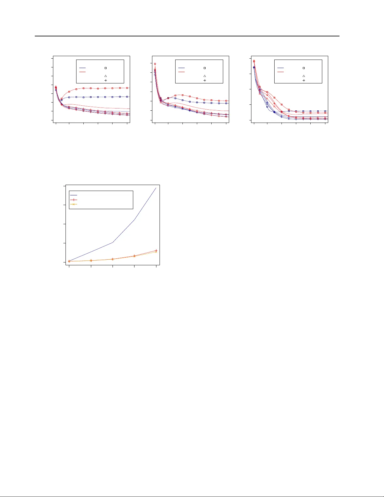
Gaussian A ppr oximation of Collective Graphical Models Li-Ping Liu 1 L I U L I @ E E C S . O R E G O N S TA T E . E D U Daniel Sheldon 2 S H E L D O N @ C S . U M A S S . E D U Thomas G. Dietterich 1 T G D @ E E C S . O R E G O N S TA T E . E D U 1 School of EECS, Oregon State Uni versity , Corvallis, OR 97331 USA 2 Univ ersity of Massachusetts, Amherst, MA 01002 and Mount Holyoke Colle ge, South Hadley , MA 01075 Abstract The Collectiv e Graphical Model (CGM) models a population of independent and identically dis- tributed individuals when only collecti ve statis- tics (i.e., counts of individuals) are observ ed. Ex- act inference in CGMs is intractable, and pre- vious work has explored Marko v Chain Monte Carlo (MCMC) and MAP approximations for learning and inference. This paper studies Gaus- sian approximations to the CGM. As the popula- tion gro ws large, we sho w that the CGM distri- bution con v erges to a multi variate Gaussian dis- tribution (GCGM) that maintains the conditional independence properties of the original CGM. If the observations are exact marginals of the CGM or marginals that are corrupted by Gaus- sian noise, inference in the GCGM approxima- tion can be computed efficiently in closed form. If the observations follo w a dif ferent noise model (e.g., Poisson), then expectation propagation pro- vides efficient and accurate approximate infer- ence. The accuracy and speed of GCGM infer- ence is compared to the MCMC and MAP meth- ods on a simulated bird migration problem. The GCGM matches or exceeds the accuracy of the MAP method while being significantly faster . 1. Introduction Consider a setting in which we wish to model the behavior of a population of independent and identically distributed (i.i.d.) individuals but where we can only observe collec- tiv e count data. For example, we might wish to model the relationship between education, sex, housing, and income from census data. For pri vac y reasons, the Census Bureau only releases count data such as the number of people ha v- Pr oceedings of the 31 st International Confer ence on Machine Learning , Beijing, China, 2014. JMLR: W&CP volume 32. Copy- right 2014 by the author(s). ing a given lev el of education or the number of men living in a particular region. Another e xample concerns modeling the behavior of animals from counts of (anonymous) indi- viduals observed at v arious locations and times. This arises in modeling the migration of fish and birds. The CGM is constructed by first defining the individual model —a graphical model describing a single indi vidual. Let C and S be the clique set and the separator set of a junc- tion tree constructed from the individual model. Then, we define N copies of this individual model to create a pop- ulation of N i.i.d. individuals. This permits us to define count v ariables n A , where n A ( i A ) is the number of indi- viduals for which clique A ∈ C ∪ S is in configuration i A . The counts n = ( n A : A ∈ C ∪ S ) are the suf ficient statis- tics of the individual model. After marginalizing away the individuals, the CGM provides a model for the joint distri- bution of n . In typical applications of CGMs, we make noisy obser - vations y that depends on some of the n variables, and we seek to answer queries about the distrib ution of some or all of the n conditioned on these observ ations. Let y = ( y D : D ∈ D ) , where D is a set of cliques from the individual graphical model and y D contains counts of set- tings of clique D . W e require each D ⊆ A for some clique A ∈ C ∪ S the indi vidual model. In addition to the usual role in graphical models, the inference of the distribution of n also serves to estimate the parameters of the indi vid- ual model (e.g. E step in EM learning), because n are suf fi- cient statistics of the individual model. Inference for CGMs is much more difficult than for the individual model. Un- like the indi vidual model, man y conditional distributions in the CGM do not have a closed form. The space of possi- ble configurations of the CGM is very large, because each count variable n i can take v alues in { 0 , . . . , N } . The original CGM paper , Sheldon and Dietterich ( 2011 ) introduced a Gibbs sampling algorithm for sampling from P ( n | y ) . Subsequent experiments showed that this exhibits slow mixing times, which motiv ated Sheldon, Sun, Kumar , and Dietterich ( 2013 ) to introduce an ef ficient algorithm Gaussian Appr oximation of Collective Graphical Models for computing a MAP approximation based on minimizing a tractable con ve x approximation of the CGM distribution. Although the MAP approximation still scales exponentially in the domain size L of the indi vidual-model v ariables, it was fast enough to permit fitting CGMs via EM on modest- sized instances ( L = 49 ). Howe v er , giv en that we wish to apply this to problems where L = 1000 , we need a method that is ev en more ef ficient. This paper introduces a Gaussian approximation to the CGM. Because the count variables n C hav e a multinomial distribution, it is reasonable to apply the Gaussian approx- imation. Howe v er , this approach raises three questions. First, is the Gaussian approximation asymptotically cor - rect? Second, can it maintain the sparse dependency struc- ture of the CGM distribution, which is critical to efficient inference? Third, how well does it work with natural (non- Gaussian) observation distributions for counts, such as the Poisson distribution? This paper answers these questions by proving an asymptotically correct Gaussian approxima- tion for CGMs. It sho ws that this approximation, when done correctly , is able to preserv e the dependency structure of the CGM. And it demonstrates that by applying expecta- tion propagation (EP), non-Gaussian observ ation distrib u- tions can be handled. The result is a CGM inference pro- cedure that gi ves good accuracy and achie ves significant speedups ov er previous methods. Beyond CGMs, our main result highlights a remarkable property of discrete graphical models: the asymptotic dis- tribution of the vector of sufficient statistics is a Gaussian graphical model with the same conditional independence properties as the original model. 2. Problem Statement and Notation Consider a graphical model defined on the graph G = ( V , E ) with n nodes and clique set C . Denote the random variables by X 1 , . . . , X n . Assume for simplicity all vari- ables take v alues in the same domain X of size L . Let x ∈ X n be a particular configuration of the variables, and let x C be the subvector of variables belonging to C . For each clique C ∈ C , let φ C ( x C ) be a non-negati ve potential function. Then the probability model is: p ( x ) = 1 Z Y C ∈C φ C ( x C ) = exp  X C ∈C X i C ∈X | C | θ C ( i C ) · I ( x C = i C ) − Q ( θ )  . (1) The second line sho ws the model in exponential-family form W ainwright & Jordan ( 2008 ), where I ( π ) is an indi- cator variable for the ev ent or expression π , and θ C ( i C ) = log φ C ( i C ) is an entry of the vector of natural parame- ters. The function Q ( θ ) = log Z is the log-partition func- tion. Gi ven a fix ed set of parameters θ and any subset A ⊆ V , the mar ginal distribution µ A is the vector with en- tries µ A ( i A ) = Pr( X A = i A ) for all possible i A ∈ X | A | . In particular , we will be interested in the clique marginals µ C and the node marginals µ i := µ { i } . Junction T r ees. Our development relies on the existence of a junction tree ( Lauritzen , 1996 ) on the cliques of C to write the rele v ant CGM and GCGM distributions in closed form. Henceforth, we assume that such a junction tree exists . In practice, this means that one may need to add fill-in edges to the original model to obtain the triangulated graph G , of which C is the set of maximal cliques. This is a clear limitation for graphs with high tree-width. Our methods apply directly to trees and are most practical for low tree- width graphs. Since we use few properties of the junction tree directly , we revie w only the essential details here and revie w the reader to Lauritzen ( 1996 ) for further details. Let C and C 0 be two cliques that are adjacent in T ; their intersection S = C ∩ C 0 is called a separator . Let S be the set of all separators of T , and let ν ( S ) be the number of times S appears as a separator , i.e., the number of dif ferent edges ( C, C 0 ) in T for which S = C ∩ C 0 . The CGM Distribution. Fix a sample size N and let x 1 , . . . , x N be N i.i.d. random vectors distributed accord- ing to the graphical model G . For an y set A ⊆ V and particular setting i A ∈ X | A | , define the count n A ( i A ) = N X m =1 I ( x m A = i A ) . (2) Let n A = ( n A ( i A ) : i A ∈ X | A | ) be the complete vector of counts for all possible settings of the variables in A . In particular , let n u := n { u } be the vector of node counts. Also, let n = ( n A : A ∈ C ∪ S ) be the combined vector of all clique and separator counts—these are sufficient statis- tics of the sample of size N from the graphical model. The distribution o ver this v ector is the CGM distribution. Proposition 1 Let n be the vector of (clique and separa- tor) sufficient statistics of a sample of size N fr om the dis- cr ete graphical model ( 1 ) . The pr obability mass function of n is given by p ( n ; θ ) = h ( n ) f ( n ; θ ) where f ( n ; θ ) = exp  X C ∈C ,i C ∈X | C | θ C ( i C ) · n C ( i C ) − N Q ( θ )  (3) Gaussian Appr oximation of Collective Graphical Models h ( n ) = N ! · Q S ∈S Q i S ∈X | S |  n S ( i S )!  ν ( S ) Q C ∈C Q i C ∈X | C | n C ( i C )! Y S ∼ C ∈T ,i S ∈X | S | I  n S ( i S ) = X i C \ S n C ( i S , i C \ S )  · Y C ∈C I  X i C ∈X | C | n C ( i C ) = N  . (4) Denote this distribution by CGM( N , θ ) . Here, the notation S ∼ C ∈ T means that S is adjacent to C in T . This proposition was first proved in nearly this form by Sundberg ( 1975 ) (see also Lauritzen ( 1996 )). Proposition 1 dif fers from those presentations by writing f ( n ; θ ) in terms of the original parameters θ instead of the clique and separator marginals { µ C , µ S } , and by includ- ing hard constraints in the base measure h ( n ) . The hard constraints enforce consistenc y of the suf ficient statistics of all cliques on their adjacent separators, and were treated implicitly prior to Sheldon & Dietterich ( 2011 ). A proof of the equiv alence between our expression for f ( n ; θ ) and the expressions from prior work is given in the supple- mentary material. Dawid & Lauritzen ( 1993 ) refer to the same distribution as the hyper-multinomial distribution due to the fact that it follows conditional independence prop- erties analogous to those in the original graphical model. Proposition 2 Let A, B ∈ S ∪ C be two sets that are sep- arated by the separ ator S in T . Then n A ⊥ ⊥ n B | n S . Proof: The probability model p ( n ; θ ) factors over the clique and separator count vectors n C and n S . The only factors where two different count vectors appear together are the consistency constraints where n S and n C appear together if S is adjacent to C in T . Thus, the CGM is a graphical model with the same structure as T , from which the claim follows.  3. A pproximating CGM by the Normal Distribution In this section, we will develop a Gaussian approximation, GCGM, of the CGM and sho w that it is the asymptoti- cally correct distribution as M goes to infinity . W e then show that the GCGM has the same conditional indepen- dence structure as the CGM, and we explicitly derive the conditional distributions. These allow us to use Gaussian message passing in the GCGM as a practical approximate inference method for CGMs. W e will follow the most natural approach of approximat- ing the CGM distribution by a multi variate Gaussian with the same mean and cov ariance matrix. The moments of the CGM distribution follow directly from those of the in- dicator variables of the individual model: Fix an outcome x = ( x 1 , . . . , x n ) from the individual model and for any set A ⊆ V let I A =  I ( x A = i A ) : i A ∈ X | A |  be the vector of all indicator variables for that set. The mean and cov ariance of any such v ectors are giv en by E [ I A ] = µ A (5) co v( I A , I B ) = h µ A,B i − µ A µ T B . (6) Here, the notation h µ A,B i refers to the matrix whose ( i A , i B ) entry is the marginal probability Pr( X A = i A , X B = i B ) . Note that Eq. ( 6 ) follo ws immediately from the definition of co variance for indicator variables, which is easily seen in the scalar form: cov( I ( X A = i A ) , I ( X B = i B )) = Pr( X A = i A , X B = i B ) − Pr( X A = i A ) Pr( X B = i B ) . Eq. ( 6 ) also covers the case when A ∩ B is nonempty . In particular if A = B = { u } , then we re- cov er cov( I u , I u ) = diag( µ u ) − µ u µ T u , which is the co- variance matrix for the marginal multinomial distribution of I u . From the preceding arguments, it becomes clear that the co- variance matrix for the full vector of indicator variables has a simple block structure. Define I = ( I A : A ∈ C ∪ S ) to be the vector concatention of all the clique and separator indi- cator variables, and let µ = ( µ A : A ∈ C ∪ S ) = E [ I ] be the corresponding vector concatenation of marginals. Then it follows from ( 6 ) that the co v ariance matrix is Σ := co v( I , I ) = ˆ Σ − µµ T , (7) where ˆ Σ is the matrix whose ( A, B ) block is the marginal distribution h µ A,B i . In the CGM model, the count vector n can be written as n = P N m =1 I m , where I 1 , . . . , I N are i.i.d. copies of I . As a result, the moments of the CGM are obtained by scaling the moments of I by N . W e thus arri ve at the natural moment-matching Gaussian approximation of the CGM. Definition 1 The Gaussian CGM, denoted GCGM( N , θ ) is the multivariate normal distribution N ( N µ , N Σ) , wher e µ is the vector of all clique and separator mar ginals of the graphical model with par ameters θ , and Σ is defined in Equation ( 7 ) . In the follo wing theorem, we show the GCGM is asymptot- ically correct and it is a Gaussian graphical model, which will lead to efficient inference algorithms. Theorem 1 Let n N ∼ CGM( N , θ ) for N = 1 , 2 , . . . . Then following ar e true: (i) The GCGM is asymptotically corr ect. That is, as N → ∞ we have 1 √ N ( n N − N µ ) D − → N ( 0 , Σ) . (8) Gaussian Appr oximation of Collective Graphical Models (ii) The GCGM is a Gaussian graphical model with the same conditional independence structure as the CGM. Let z ∼ GCGM( N , θ ) and let A, B ∈ C ∪ S be two sets that ar e separated by separator S in T . Then z A ⊥ ⊥ z B | z S . Proof: P art (i) is a direct application of the multiv ariate central limit theorem to the random vector n N , which, as noted above, is a sum of i.i.d. random vectors I 1 , . . . , I N with mean µ and cov ariance Σ ( Feller , 1968 ). Part (ii) is a consequence of the fact that these conditional independence properties hold for each n N (Proposition 2 ), so they also hold in the limit as N → ∞ . While this is intu- itiv ely clear , it seems to require further justification, which is provided in the supplementary material.  3.1. Conditional Distributions The goal is to use inference in the GCGM as a tractable ap- proximate alternati ve inference method for CGMs. How- ev er , it is very dif ficult to compute the co variance matrix Σ ov er all cliques. In particular , note that the ( C, C 0 ) block requires the joint marginal h µ C,C 0 i , and if C and C 0 are not adjacent in T this is hard to compute. F ortunately , we can sidestep the problem completely by le veraging the graph structure from Part (ii) of Theorem 1 to write the distribu- tion as a product of conditional distrib utions whose param- eters are easy to compute (this effecti vely means working with the inv erse covariance matrix instead of Σ ). W e then perform inference by Gaussian message passing on the re- sulting model. A challenge is that Σ is not full rank, so the GCGM distri- bution as written is degenerate and does not have a den- sity . This can be seen by noting that any vector n ∼ CGM( N ; θ ) with nonzero probability satisfies the affine consistency constraints from Eq. ( 4 )—for example, each vector n C and n S sums to the population size N —and that these affine constraints also hold with probability one in the limiting distribution. T o fix this, we instead use a linear transformation T to map z to a reduced vector ˜ z = T z such that the reduced co v ariance matrix ˜ Σ = T Σ T T is in- vertible. The work by Loh & W ainwright ( 2013 ) proposed a minimal representation of the graphical model in ( 1 ), and the corresponding random variable has a full rank cov ari- ance matrix. W e will find a transformation T to project our indicator variable I into that form. Then T I (as well as T n and T z ) will have a full rank co variance matrix. Denote by C + the maximal and non-maximal cliques in the triangulated graph. Note that each D ∈ C + must be a sub- set of some A ∈ C ∪ S and each subset of A is also a clique in C + . For every D ∈ C + , let X D 0 = ( X \{ L } ) | D | denote the space of possible configurations of D after excluding the largest value, L , from the domain of each variable in D . The corresponding random variable I in the minimal representation is defined as ( Loh & W ainwright , 2013 ): ˜ I = ( I ( x D = i D ) : i D ∈ X D 0 , D ∈ C + ) . (9) ˜ I D can be calculated linearly from I A when D ⊆ A via the matrix T D,A whose ( i D , i A ) entry is defined as T D,A ( i D , i A ) = I ( i D ∼ D i A ) , (10) where ∼ D means that i D and i A agree on the setting of the variables in D . It follo ws that ˜ I D = T D,A I A . The whole transformation T can be built in blocks as follows: For ev ery D ∈ C + , choose A ∈ C ∪ S and construct the T D,A block via ( 10 ). Set all other blocks to zero. Due to the redundancy of I , there might be many ways of choosing A for D and any one will work as long as D ⊆ A . Proposition 3 Define T as above, and define ˜ z = T z , ˜ z A + = ( ˜ z D : D ⊆ A ) , A ∈ C ∪ S . Then (i) If A, B ∈ C ∪ S ar e separated by S in T , it holds that ˜ z A + ⊥ ⊥ ˜ z B + | ˜ z S + . (ii) The covariance matrix of ˜ z has full rank. Proof: In the appendix, we sho w that for an y A ∈ C ∪ S , I A can be linearly recovered from ˜ I A + = ( ˜ I D : D ⊆ A ) . So there is a linear bijection between I A and ˜ I A + (The mapping from I A to ˜ I A + has been sho wn in the defini- tion of T ). The same linear bijection relation also exists between n A and ˜ n A + = P N m =1 ˜ I m A + and between z A and ˜ z A + . Proof of (i): Since z A ⊥ ⊥ z B | z S , it follows that ˜ z A + ⊥ ⊥ ˜ z B + | z S because ˜ z A + and ˜ z B + are deterministic functions of z A and z B respectiv ely . Since z S is a deterministic func- tion of ˜ z S + , the same property holds when we condition on ˜ z S + instead of z S . Proof of (ii): The bijection between I and ˜ I indicates that the model representation of Loh & W ainwright ( 2013 ) de- fines the same model as ( 1 ). By Loh & W ainwright ( 2013 ), ˜ I has full rank cov ariance matrix and so do ˜ n and ˜ z .  W ith this result, the GCGM can be decomposed into conditional distributions, and each distribution is a non- degenerate Gaussian distrib ution. Now let us consider the observ ations y = { y D , D ∈ D} , where D is the set of cliques for which we hav e observ a- tions. W e require each D ∈ D be subset of some clique C ∈ C . When choosing a distribution p ( y D | z C ) , a mod- eler has substantial flexibility . For example, p ( y D | z C ) can be noiseless, y D ( i D ) = P i C \ D z C ( i D , i C \ D ) , which permits closed-form inference. Or p ( y D | z C ) can con- sist of independent noisy observations: p ( y D | z C ) = Q i D p ( y D ( i D ) | P i C \ D z C ( i D , i C \ D )) . With a little work, p ( y D | z C ) can be represented by p ( y D | ˜ z C + ) . Gaussian Appr oximation of Collective Graphical Models 3.2. Explicit Factor ed Density f or T rees W e describe how to decompose GCGM for the special case when the original graphical model G is a tree. W e assume that only counts of single nodes are observed. In this case, we can marginalize out edge (clique) counts z { u,v } and re- tain only node (separator) counts z u . Because the GCGM has a normal distribution, marginalization is easy . The con- ditional distribution is then defined only on node counts. W ith the definition of ˜ z in Proposition ( 3 ) and the property of conditional independence, we can write p ( ˜ z 1 , . . . , ˜ z n ) = p ( ˜ z r ) Y ( u,v ) ∈ E p ( ˜ z v | ˜ z u ) . (11) Here r ∈ V is an arbitrarily-chosen root node, and E is the set of dir ected edges of G oriented away from r . The marginalization of the edges greatly reduces the size of the inference problem, and a similar technique is also applica- ble to general GCGMs. Now specify the parameters of the Gaussian conditional densities p ( ˜ z v | ˜ z u ) in Eq. ( 11 ). Assume the blocks T u,u and T v ,v are defined as ( 10 ). Let ˜ µ u = T u,u µ u be the marginal vector of node u without its last entry , and let h ˜ µ u,v i = T u,u h µ u,v i T T v ,v be the marginal matrix o ver edge ( u, v ) , minus the final ro w and column. Then the mean and cov ariance martix of the joint distribution are η := N  ˜ µ u ˜ µ v  , N 2  diag( ˜ µ u ) h ˜ µ u,v i h ˜ µ v ,u i diag ( ˜ µ v )  − η η T . (12) The conditional density p ( ˜ z v | ˜ z u ) is obtained by standard Gaussian conditioning formulas. If we need to infer z { u,v } from some distribution q ( ˜ z u , ˜ z v ) , we first calculate the distribution p ( ˜ z { u,v } | ˜ z u , ˜ z v ) . This time we assume blocks T { u,v } + , { u,v } = ( T u, { u,v } : D ∈ { u, v } ) are defined as ( 10 ). W e can find the mean and variance of p ( ˜ z u , ˜ z v , ˜ z { u,v } ) by applying linear transfor- mation T { u,v } + , { u,v } on the mean and v ariance of z { u,v } . Standard Gaussian conditioning formulas then giv e the conditional distribution p ( ˜ z { u,v } | ˜ z u , ˜ z v ) . Then we can recov er the distribution of z { u,v } from distrib ution p ( ˜ z { u,v } | ˜ z u , ˜ z v ) q ( ˜ z u , ˜ z v ) . Remark: Our reasoning giv es a completely different way of deriving some of the results of Loh & W ainwright ( 2013 ) concerning the sparsity pattern of the in verse cov ariance matrix of the sufficient statistics of a discrete graphical model. The conditional independence in Proposition 2 for the factored GCGM density translates directly to the spar- sity pattern in the precision matrix Γ = ˜ Σ − 1 . Unlike the reasoning of Loh & W ainwright , we derive the sparsity di- rectly from the conditional independence properties of the asymptotic distribution (which are inherited from the CGM distribution) and the fact that the CGM and GCGM share the same cov ariance matrix. 4. Inference with Noisy Obser vations W e now consider the problem of inference in the GCGM when the observations are noisy . Throughout the remainder of the paper , we assume that the individual model—and, hence, the CGM—is a tree. In this case, the cliques cor- respond to edges and the separators correspond to nodes. W e will also assume that only the nodes are observed. For notational simplicity , we will assume that ev ery node is ob- served (with noise). (It is easy to mar ginalize out unob- served nodes if any .) From now on, we use uv instead of { u, v } to represent edge clique. Finally , we assume that the entries hav e been dropped from the vector z as described in the previous section so that it has the factored density described in Eq. 11 . Denote the observation variable for node u by y u , and as- sume that it has a Poisson distribution. In the (exact) CGM, this would be written as y u ∼ P oisson( n u ) . Ho wev er , in our GCGM, this instead has the form y u ∼ Poisson( λ z u ) , (13) where z u is the corresponding continuous v ariable and λ determines the amount of noise in the distribution. Denote the vector of all observations by y . Note that the missing entry of z u must be reconstructed from the remaining en- tries when computing the likelihood. W ith Poisson observations, there is no longer a closed-form solution to message passing in the GCGM. W e address this by applying Expectation Propagation (EP) with the Laplace approximation. This method has been previously applied to nonlinear dynamical systems by Ypma and Heskes ( 2005 ). 4.1. Inferring Node Counts In the GCGM with observations, the potential on each edge ( u, v ) ∈ E is defined as ψ ( z u , z v ) =  p ( z v , z u ) p ( y v | z v ) p ( y u | z u ) if u is root p ( z v | z u ) p ( y v | z v ) otherwise. (14) W e omit the subscripts on ψ for notational simplicity . The joint distribution of ( z v , z u ) has mean and cov ariance shown in ( 12 ). W ith EP , the model approximates potential on edge ( u, v ) ∈ E with normal distribution in context q \ uv ( z u ) and q \ uv ( z v ) . The context for edge ( u, v ) is defined as q \ uv ( z u ) = Y ( u,v 0 ) ∈ E ,v 0 6 = v q uv 0 ( z u ) (15) q \ uv ( z v ) = Y ( u 0 ,v ) ∈ E ,u 0 6 = u q u 0 v ( z v ) , (16) Gaussian Appr oximation of Collective Graphical Models where each q uv 0 ( z u ) and q u 0 v ( z v ) hav e the form of normal densities. Let ξ ( z u , z v ) = q \ uv ( z u ) q \ uv ( z v ) ψ ( z u , z v ) . The EP up- date of q uv ( z u ) and q uv ( z v ) is computed as q uv ( z u ) = pro j z u [ ξ ( z u , z v )] q \ uv ( z u ) (17) q uv ( z v ) = pro j z v [ ξ ( z u , z v )] q \ uv ( z v ) . (18) The projection operator , pro j , is computed in tw o steps. First, we find a joint approximating normal distribution via the Laplace approximation and then we project this onto each of the random v ariables z u and z v . In the Laplace ap- proximation step, we need to find the mode of log ξ ( z u , z v ) and calculate its Hessian at the mode to obtain the mean and variance of the approximating normal distrib ution: µ ξ uv = arg max ( z u , z v ) log ξ ( z u , z v ) (19) Σ ξ uv = ∇ 2 ( z u , z v )= µ ξ uv log ξ ( z u , z v ) ! − 1 . (20) The optimization problem in ( 19 ) is solved by optimizing first over z u then over z v . The optimal value of z u can be computed in closed form in terms of z v , since only nor- mal densities are in v olved. Then the optimal v alue of z v is found via gradient methods (e.g., BFGS). The function log ξ ( z u , z v ) is concave, so we can always find the global optimum. Note that this decomposition approach only de- pends on the tree structure of the model and hence will work for any observ ation distrib ution. At the mode, we find the mean and variance of the normal distribution approximating p ( z u , z v | y ) via ( 19 ) and ( 20 ). W ith this distribution, the edge counts can be inferred with the method of Section 3.2 . In the projection step in ( 17 ) and ( 18 ), this distrib ution is projected to one of z u or z v by marginalizing out the other . 4.2. Complexity analysis What is the computational comple xity of inference with the GCGM? When inferring node counts, we must solve the optimization problem and compute a fixed number of matrix inv erses. Each matrix in verse takes time L 2 . 5 . In the Laplace approximation step, each gradient calculation takes O ( L 2 ) time. Suppose m iterations are needed. In the outer loop, suppose we must perform r passes of EP mes- sage passing and each iteration sweeps through the whole tree. Then the o verall time is O ( r | E | max( mL 2 , L 2 . 5 )) . The maximization problem in the Laplace approximation is smooth and concav e, so it is relati vely easy . In our ex- periments, EP usually con ver ges within 10 iterations. In the task of inferring edge counts, we only consider the complexity of calculating the mean, as this is all that is needed in our applications. This part is solved in closed form, with the most time-consuming operation being the matrix inv ersion. By exploiting the simple structure of the cov ariance matrix of z uv , we can obtain an inference method with time complexity of O ( L 3 ) . 5. Experimental Evaluation In this section, we e valuate the performance of our method and compare it to the MAP approximation of Sheldon, Sun, Kumar , and Dietterich ( 2013 ). The e v aluation data are gen- erated from the bird migration model introduced in Shel- don et al. ( 2013 ). This model simulates the migration of a population of M birds on an L = ` × ` map. The entire population is initially located in the bottom left corner of the map. Each bird then makes independent migration de- cisions for T = 20 time steps. The transition probability from cell i to cell j at each time step is determined by a lo- gistic regression equation that employs four features. These features encode the distance from cell i to cell j , the degree to which cell j falls near the path from cell i to the destina- tion cell in the upper right corner, the degree to which cell j lies in the direction toward which the wind is blowing, and a factor that encourages the bird to stay in cell i . Let w denote the parameter vector for this logistic regression for - mula. In this simulation, the indi vidual model for each bird is a T -step Marko v chain X = ( X 1 , . . . , X 20 ) where the domain of each X t consists of the L cells in the map. The CGM variables n = ( n 1 , n 1 , 2 , n 2 , . . . , n T ) are vectors of length L containing counts of the number of birds in each cell at time t and the number of birds mo ving from cell i to cell j from time t to time t + 1 . W e will refer to these as the “node counts” (N) and the “edge counts” (E). At each time step t , the data generation model generates an obser- vation vector y t of length L which contains noisy counts of birds at all map cells at time t , n t . The observed counts are generated by a Poisson distribution with unit intensity . W e consider two inference tasks. In the first task, the pa- rameters of the model are giv en, and the task is to infer the expected value of the posterior distribution over n t for each time step t gi ven the observations y 1 , . . . , y T (aka “smoothing”). W e measure the accuracy of the node counts and edge counts separately . An important experimental issue is that we cannot com- pute the true MAP estimates for the node and edge counts. Of course we ha ve the v alues generated during the sim- ulation, but because of the noise introduced into the ob- servations, these are not necessarily the expected values of the posterior . Instead, we estimate the expected v al- ues by running the MCMC method ( Sheldon & Dietterich , 2011 ) for a b urn-in period of 1 million Gibbs iterations Gaussian Appr oximation of Collective Graphical Models and then collecting samples from 10 million Gibbs iter - ations and averaging the results. W e ev aluate the ac- curacy of the approximate methods as the relati ve error || n app − n mcmc || 1 / || n mcmc || 1 , where n app is the approx- imate estimate and n mcmc is the value obtained from the Gibbs sampler . In each e xperiment, we report the mean and standard deviation of the relativ e error computed from 10 runs. Each run generates a new set of values for the node counts, edge counts, and observation counts and requires a separate MCMC baseline run. W e compare our method to the approximate MAP method introduced by Sheldon et al. ( 2013 ). By treating counts as continuous and approximating the log factorial function, their MAP method finds the approximate mode of the pos- terior distribution by solving a con ve x optimization prob- lem. Their work shows that the MAP method is much more efficient than the Gibbs sampler and produces inference re- sults and parameter estimates very similar to those obtained from long MCMC runs. The second inference task is to estimate the parameters w of the transition model from the observations. This is per- formed via Expectation Maximization, where our GCGM method is applied to compute the E step. W e compute the relativ e error with respect to the true model parameters. T able 1 compares the inference accuracy of the approxi- mate MAP and GCGM methods. In this table, we fixed L = 36 , set the logistic regression coefficient vector w = (1 , 2 , 2 , 2) , and v aried the population size N ∈ { 36 , 360 , 1080 , 3600 } . At the smallest population size, the MAP approximation is slightly better , although the result is not statistically significant. This makes sense, since the Gaussian approximation is weakest when the population size is small. At all larger population sizes, the GCGM giv es much more accurate results. Note that the MAP ap- proximation exhibits much higher v ariance as well. T able 1. Relativ e error in estimates of node counts (“N”) and edge counts (“E”) for different population sizes N . N = 36 360 1080 3600 MAP(N) .173 ± .020 .066 ± .015 .064 ± .012 .069 ± .013 MAP(E) .350 ± .030 .164 ± .030 .166 ± .027 .178 ± .025 GCGM(N) .184 ± .018 .039 ± .007 .017 ± .003 .009 ± .002 GCGM(E) .401 ± .026 .076 ± .008 .034 ± .003 .017 ± .002 Our second inference experiment is to vary the magnitude of the logistic regression coefficients. W ith large coeffi- cients, the transition probabilities become more e xtreme (closer to 0 and 1), and the Gaussian approximation should not work as well. W e fixed N = 1080 and L = 36 and ev aluated three different parameter vectors: w 0 . 5 = (0 . 5 , 1 , 1 , 1) , w 1 = (1 , 2 , 2 , 2) and w 2 = (2 , 4 , 4 , 4) . T a- ble 2 sho ws that for w 0 . 5 and w 1 , the GCGM is much more accurate, b ut for w 2 , the MAP approximation gi ves a slightly better result, although it is not statistically signifi- cant based on 10 trials. T able 2. Relativ e error in estimates of node counts (“N”) and edge counts (“E”) for different settings of the logistic regression param- eter vector w w 0 . 5 w 1 w 2 MAP(N) .107 ± .014 .064 ± .012 .018 ± .004 MAP(E) .293 ± .038 .166 ± .027 .031 ± .004 GCGM(N) .013 ± .002 .017 ± .003 .024 ± .004 GCGM(E) .032 ± .004 .034 ± .003 .037 ± .005 Our third inference experiment explores the effect of vary- ing the size of the map. This increases the size of the do- main for each of the random variables and also increases the number of values that must be estimated (as well as the amount of evidence that is observed). W e vary L ∈ { 16 , 25 , 36 , 49 } . W e scale the population size accordingly , by setting N = 30 L . W e use the coefficient vector w 1 . The results in T able 3 sho w that for the smallest map, both methods gi ve similar results. But as the number of cells grows, the relative error of the MAP approximation grows rapidly as does the variance of the result. In comparison, the relativ e error of the GCGM method barely changes. T able 3. Relativ e inference error with different map size L = 16 25 36 49 MAP(N) .011 ± .005 .025 ± .007 .064 ± .012 .113 ± .015 MAP(E) .013 ± .004 .056 ± .012 .166 ± .027 .297 ± .035 GCGM(N) .017 ± .003 .017 ± .003 .017 ± .003 .020 ± .003 GCGM(E) .024 ± .002 .027 ± .003 .034 ± .003 .048 ± .005 W e now turn to measuring the relativ e accuracy of the methods during learning. In this experiment, we set L = 16 and v ary the population size for N ∈ { 16 , 160 , 480 , 1600 } . After each EM iteration, we compute the relativ e error as || w lear n − w true || 1 / || w true || 1 , where w lear n is the param- eter vector estimated by the learning methods and w true is the parameter vector that was used to generate the data. Figure 1 sho ws the training curves for the three parame- ter vectors w 0 . 5 , w 1 , and w 2 . The results are consistent with our previous experiments. F or small population sizes ( N = 16 and N = 160 ), the GCGM does not do as well as the MAP approximation. In some cases, it overfits the data. For N = 16 , the MAP approximation also exhibits over - fitting. F or w 2 , which creates extreme transition probabil- ities, we also observe that the MAP approximation learns faster , although the GCGM eventually matches its perfor- mance with enough EM iterations. Our final experiment measures the CPU time required to perform inference. In this experiment, we varied L ∈ { 16 , 36 , 64 , 100 , 144 } and set N = 100 L . W e used pa- rameter vector w 1 . W e measured the CPU time consumed to infer the node counts and the edge counts. The MAP Gaussian Appr oximation of Collective Graphical Models 0.0 0.1 0.2 0.3 0.4 0.5 0.6 0.7 w = (0.5, 1, 1, 1) EM iteration relative error ● ● ● ● ● ● ● ● ● ● ● ● ● ● ● ● ● ● ● ● ● ● 1 10 20 30 40 50 ● population size 16 160 480 1600 methods MAP GCGM 0.0 0.1 0.2 0.3 0.4 0.5 0.6 w = (1, 2, 2, 2) EM iteration relative error ● ● ● ● ● ● ● ● ● ● ● ● ● ● ● ● ● ● ● ● ● ● 1 10 20 30 40 50 ● population size 16 160 480 1600 methods MAP GCGM 0.0 0.2 0.4 0.6 0.8 w = (2, 4, 4, 4) EM iteration relative error ● ● ● ● ● ● ● ● ● ● ● ● ● ● ● ● ● ● ● ● ● ● 1 10 20 30 40 50 ● population size 16 160 480 1600 methods MAP GCGM Figure 1. EM con ver gence curve dif ferent feature coef ficient and population sizes ● ● ● ● ● 0 20 40 60 80 Inference time v.s. domain size domain size running time (seconds) 16 36 64 100 144 ● MAP GCGM GCGM infer node counts only Figure 2. A comparison of inference run time with different num- bers of cells L method infers the node and edge counts jointly , whereas the GCGM first infers the node counts and then computes the edge counts from them. W e report the time required for computing just the node counts and also the total time required to compute the node and edge counts. Figure 2 shows that the running time of the MAP approximation is much larger than the running time of the GCGM approx- imation. For all values of L except 16, the a verage run- ning time of GCGM is more than 6 times faster than for the MAP approximation. The plot also re veals that the computation time of GCGM is dominated by estimating the node counts. A detailed analysis of the implementa- tion indicates that the Laplace optimization step is the most time-consuming. In summary , the GCGM method achiev es relativ e error that matches or is smaller than that achie ved by the MAP ap- proximation. This is true both when measured in terms of estimating the values of the latent node and edge counts and when estimating the parameters of the underlying graphi- cal model. The GCGM method does this while running more than a factor of 6 faster . The GCGM approxima- tion is particularly good when the population size is large and when the transition probabilities are not near 0 or 1. Con versely , when the population size is small or the prob- abilities are extreme, the MAP approximation gives better answers although the differences were not statistically sig- nificant based on only 10 trials. A surprising finding is that the MAP approximation has much lar ger variance in its an- swers than the GCGM method. 6. Concluding Remarks This paper has introduced the Gaussian approximation (GCGM) to the Collecti ve Graphical Model (CGM). W e hav e shown that for the case where the observations only depend on the separators, the GCGM is the limiting dis- tribution of the CGM as the population size N → ∞ . W e showed that the GCGM cov ariance matrix maintains the conditional independence structure of the CGM, and we presented a method for efficiently in verting this cov ari- ance matrix. By applying expectation propagation, we de- veloped an ef ficient algorithm for message passing in the GCGM with non-Gaussian observ ations. Experiments on a bird migration simulation showed that the GCGM method is at least as accurate as the MAP approximation of Shel- don et al. ( 2013 ), that it exhibits much lower variance, and that it is 6 times faster to compute. Acknowledgement This material is based upon work supported by the National Science Foundation under Grant No. 1125228. Gaussian Appr oximation of Collective Graphical Models References Dawid, A. P . and Lauritzen, S. L. Hyper Markov laws in the statistical analysis of decomposable graphical mod- els. The Annals of Statistics , 21(3):1272–1317, 1993. Feller , W . An Intr oduction to Pr obability Theory and Its Applications, V ol. 2 . W ile y , 1968. Lauritzen, S.L. Graphical models . Oxford Univ ersity Press, USA, 1996. Loh, Po-Ling and W ainwright, Martin J. Structure estima- tion for discrete graphical models: Generalized cov ari- ance matrices and their in verses. The Annals of Statistics , 41(6):3022–3049, 2013. Sheldon, Daniel and Dietterich, Thomas G. Collectiv e Graphical Models. In NIPS 2011 , 2011. Sheldon, Daniel, Sun, T ao, Kumar , Akshat, and Dietterich, Thomas G. Approximate Inference in Collecti ve Graph- ical Models. In Pr oceedings of ICML 2013 , pp. 9, 2013. Sundberg, R. Some results about decomposable (or Markov-type) models for multidimensional contingency tables: distribution of mar ginals and partitioning of tests. Scandinavian Journal of Statistics , 2(2):71–79, 1975. W ainwright, M.J. and Jordan, M.I. Graphical models, ex- ponential families, and v ariational inference. F ounda- tions and T rends in Machine Learning , 1(1-2):1–305, 2008. Ypma, Alexander and Heskes, T om. Novel approximations for inference in nonlinear dynamical systems using ex- pectation propagation. Neur ocomputing , 69(1-3):85–99, 2005. Gaussian Appr oximation of Collective Graphical Models A. Proof of Pr oposition 1 The usual way of writing the CGM distribution is to replace f ( n ; θ ) in Eq. ( 3 ) by f 0 ( n ; θ ) = Q C ∈C ,i C ∈X | C | µ C ( i C ) n C ( i C ) Q S ∈S ,i S ∈X | S |  µ S ( i S ) n S ( i S )  ν ( S ) (21) W e will show that f ( n ; θ ) = f 0 ( n ; θ ) for any n such that h ( n ) > 0 by showing that both descibe the probability of an ordered sample with sufficient statistics n . Indeed, sup- pose there exists some ordered sample X = ( x 1 , . . . , x N ) with sufficient statistics n . Then it is clear from inspection of Eq. ( 3 ) and Eq. ( 21 ) that f ( n ; θ ) = Q N m =1 p ( x m ; θ ) = f 0 ( n ; θ ) by the junction tree reparameterization of p ( x ; θ ) ( W ainwright & Jordan , 2008 ). It only remains to sho w that such an X exists whenever h ( n ) > 0 . This is exactly what was shown by Sheldon & Dietterich ( 2011 ): for junction trees, the hard constraints of Eq. ( 4 ), which enforce local consistency on the integer count variables, are equiv alent to the global consistency property that there exists some or - dered sample X with sufficient statistics equal to n . (Since these are integer count variables, the proof is quite dif fer- ent from the similar theorem that local consistency implies global consistency for marginal distributions.) W e briefly note two interesting corollaries to this argument. First, by the same reasoning, any reparameterization of p ( x ; θ ) that factors in the same way can be used to replace f ( n ; θ ) in the CGM distrib ution. Second, we can see that the base measure h ( n ) is exactly the number of differ ent or der ed samples with sufficient statistics equal to n . B. Proof of Theor em 1 : Additional Details Suppose { n N } is a sequence of random vectors that con- ver ge in distribution to n , and that n N A , n N B , and n N S are subv ectors that satisfy n N A ⊥ ⊥ n N B | n N S (22) for all N . Let α , β , and γ be measurable sets in the appro- priate spaces and define z = Pr( n A ∈ α, n B ∈ β | n S ∈ γ ) − (23) Pr( n A ∈ α | n S ∈ γ ) Pr( n B ∈ β | n S ∈ γ ) Also let z N be the same expression but with all instances of n replaced by n N and note that z N = 0 for all N by the as- sumed conditional independence property of Eq. ( 22 ). Be- cause the sequence { n N } con ver ges in distribution to n , we hav e conv ergence of each term in z N to the corresponding term in z , which means that z = lim N →∞ z N = lim N →∞ 0 = 0 , so the conditional independence property of Eq. ( 22 ) also holds in the limit. C. Proof of Theor em 3 : Linear Function fr om ˜ I to I W e need to show I A can be recov ered from ˜ I A + with a linear function. Suppose the last indicator variable in I A is i 0 A , which cor- responds to the setting that all nodes in A take value L . Let I 0 A be a set of indicators which contains all entries in I A but the last one i 0 A . Then I A can be recovered from I 0 A by the constraint P i A I A ( i A ) = 1 . Now we only need to show that I 0 A can be recovered from I A + linearly . W e claim that there exists an in vertible matrix H such that H I 0 A = ˜ I A + . Showing the existence of H . Let ˜ I A + ( i D ) be the i D entry of ˜ I A + , which is for configuration i D of clique D , D ⊆ A . ˜ I A + ( i D ) = X i A \ D I 0 A ( i D , i A \ D ) (24) Since no nodes in D take value L by definition of ˜ I D , ( i D , i A \ D ) cannot be the missing entry i 0 A of I 0 A , and the equation is always v alid. Showing that H is square. For each D , there are ( L − 1) | D | entries, and A has  | A | | D |  sub-cliques with size | D | . So ˜ I A + hav e overall L | A | − 1 entries, which is the same as I 0 A . So H is a square matrix. W e view I 0 A and ˜ I A + as matrices and each ro w is a indi- cator function of graph configurations. Since no trivial lin- ear combination of ˜ I A + is a constant by the conclusion in Loh and W ainwright ( 2013 ), ˜ I A + has linearly independent columns. Therefore, H must have full rank and I 0 A must hav e linearly independent columns.