Modelling Data Dispersion Degree in Automatic Robust Estimation for Multivariate Gaussian Mixture Models with an Application to Noisy Speech Processing

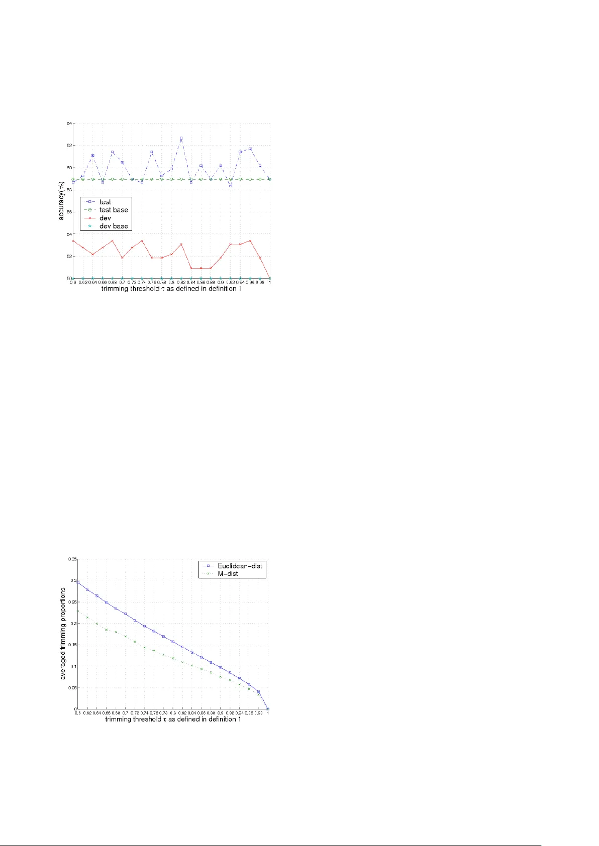
Advance s in Appl ied Acoustic s (AIAA) V ol ume 2 Is s ue 1, February 201 3 www.a iaa - journal.o rg 1 Modelli ng Data Dispe rsion Degre e in Automati c Ro bust Est imation f or Mu ltivari ate Gaussian Mixture M odels with an Applic ation to Noisy Speec h Process ing Dalei Wu *1 , Hai qing W u 2 Department of Electrical and Computer Eng ineering, Concordia University 1455 Ma isonneuv e Blvd. West, Montreal, QC H 3G 1M8, Canada *1 dale iwu@ gma il.com ; 2 ha iqin gwu @gma il.com Ab s tract The trim ming schem e with a prefixe d cut off portion is known as a me thod o f impro ving the ro bust ness of stat istic al models such a s multivar iate Ga ussia n mixture models ( MG - MMs) in small sc ale tests b y alleviating the impacts o f outliers. However, when this metho d is applied to real - world data , such as noisy spee ch processing, it is ha rd to kn ow t he opti ma l c ut - off po rtion to remov e the o utlie rs and some ti m es removes useful data samples as well. In t his paper, we pro pose a new me thod based o n measuri ng the dispersio n degre e (DD) o f the t raining d ata to avoi d this pr oble m , so as to realise automatic r obust e stima tion fo r MGMMs. The DD mode l is st udied by usin g two d if ferent measures. For each o ne , we the oretica lly prove th at the DD of the data samples in a co ntext of MGMMs approximately obeys a sp ecific (ch i or chi - square) distributio n. The proposed method is e valuated o n a real - wo rld application with a m odera tely - sized speaker re cognit ion t ask. Experime nts sho w that t he pro po sed metho d can signific antly impro ve the ro bus tness o f the co nvent ional training method o f GMMs for speaker recognitio n . Keywor ds Gaussian Mix ture Models ; K- mean s; Tri mmed K - mean s; Speech P rocessing Introd ucti on Sta tist ica l mode ls, su ch as Ga uss ian M ixture M ode ls (GMMs) [17] and H idden Ma rkov M odels (HMMs) [15 ], are impo rtant te chnique s in many signa l proc essi ng domai ns, whi ch i nclud e, for ins tance, acoustic al noi se reductio n [20], image r ec ogni tio n [8] , speech/speaker recogn ition [15, 19, 25], etc. In this paper, we study a rob ust modelling issue regarding GMMs. This issue is importa nt, since GMMs are often used a s fundame ntal compo nents to build some mo re compl icated mo dels, suc h as HMMs. Thus, t he me tho d studied in this pa per will be useful for other models as well. The sta ndard tr aini ng met hod f or GMM s is M axi mu m like lih ood E stimation ( MLE) [2] b ased on the E xpe ct ati o n M ax imisation (EM) algor ithm [4]. Th ough it has been proved effective, this m eth od st ill la cks robustness in i ts traini ng pro cess. Fo r instance, it is no t robust agai nst gross outl iers and canno t compensate the impacts fr om the out - l iers co ntai ned in a train ing corpus. As i t i s well known, o utlier s often widel y exist in a tr aining po pulation, due to the cl ean data often either being con taminated by noise, or interfered by the obj ects o ther tha n the cl aim ed d ata. O ut - l iers in the training pop ulatio n may distract the par ameters o f the trained models to inappropriate locat ions [ 3 ] and ca n therefore brea k the models down and resul t in p oor perform - ance of a rec ognition sys tem. In order to s olve this problem, a partial trimming scheme is introduced by Cuesta et al [ 3] to i mprove the robustne ss of the sta tis tica l mod els, s uch as K -m eans an d GMMs. In their method, a prefixed proportion of dat a samples is removed from th e training corpus an d the rest of th e data are us ed for model training . This method ha s been found ro bust ag ainst gross ou tliers when i t is appl ie d to smal l scal e dat a examples. However, when this method is used in real - wo rld appli - cati ons, such a s noisy acousti c sign al pro cessing, it is har d to kn ow th e optim al cu toff p roport ion that should be used, since one do es not kn ow what fa ction of the data sho ul d be tak e n aw ay f rom the overall tra inin g pop ula tion. A bigger or smaller remova l proport ion would result i n either removing too much useful inf ormati on o r having no ef fect o n remov - ing outliers. To atta ck this issue, we propose a new method b y using a dispersion deg ree mo del wi th two www.ai aa - jou rnal.org Advances in Appli ed Acoustics (AI AA) V ol ume 2 Iss ue 1, Februa ry 201 3 2 different dista nce metrics to ident ify the outlier s autom ati cal ly. The c ontr ibution s of our proposed method a re three - fold: F irst, w e suggest to use the trimmed K - me ans algorithm to rep lace the conv entional K - means app roa ch to in itia lise the p aram eters of GMMs. It is showed in thi s paper th at ap propr iat e init ial v alu es for model parameters are crucial for the robust training of GMMs. Sec ond, we propose to use t he dispersion degree of the t raining da ta samples as a selection criterion for aut omatic outlier removal. We theoretically prov e that the dispersion degre e approximately ob eys a certain distrib ution, depending on the measu re it uses. We refer this method a s the automatic r obust estimati on with a tri mmi ng sche me (ARE - TRIM) fo r Gaussi an mi x ture models hereafter. Third, we evaluate th e pro posed method on a real - world app lica tion with a m oder ate ly - sized spe aker recognition tas k. The experimental resu lts show that the proposed meth od can significantly impr ove the robu stne ss of th e conv entiona l tra inin g alg orith m for GMMs by making i t more r obust ag ainst gro ss outl ier s. The rest of th is paper is orga nised as follows: In Section 2, we presen t the fra mework of our proposed ARE - T RIM trai ning alg ori thm for GM Ms. In Sec tio n 3, we present t he trimmed K - means clust ering al gori thm and comp are i t with t he convent io nal K - means. In Section 4, we propose the dispersion degree mode l based on tw o distance metrics and use it for ARM - TRIM. We carry out th e experiments to evaluate ARE - TRI M in S ection 5 an d fin ally we conclude th is paper with o ur fi ndings i n Se ction 6 . Frame wor k of Aut oma tic Tr immin g Algori thm for Ga ussi an Mixt ur e Mod els The proposed ARE - TR IM alg orith m e ssen tia lly inclu des sev era l mod ifica t ions t o th e c onv ent iona l tra ini ng metho d o f GMMs. The co nventi onal GM M tra inin g a lgorit hm norm - all y consi sts of two steps: th e K- means clustering algorithm for model param eter init ialis at ion 1 1 Som e othe r mo del in iti alis atio n me thods ex ist, s uch as m ixtu re split ting , but the in it ialis atio n with K - mea ns is com parab le in performa nc e to the oth ers and al so more popul ar. S o we stic k to K - means. and the EM algorithm for pa rameter fine tr ain ing, as illust rat ed in Fig. 1. It i s well known that app ropr iate initia l v alue s for model parameters crucially affect the f inal performance of G MMs [2]. Inapp - ropriate initial va lues could cause the fine training with EM at the second step to be trapped at a loca l opt imu m, w hic h is of ten not g lob ally opt ima l. Therefore, it is interes ting to study more ro bust clus terin g a lgorit hm s to h elp tr ain better m odel parameters. FIG. 1 THE CONVEN TIONA L TRA INING ALGO RITHM FOR GMMS The ARE - TRI M is f ocused o n modi fying the f irst stag e of the conventiona l GMM training algorithm, i.e., the model p arameter initia lisation algorithm, b ut keeping the fi ne trai ning s tep wi th EM u ntouche d. The modifi catio n consists o f two st eps: (1 ) substitut ing fo r the co nventi onal K - means c lust ering alg orith m b y a more robust trimmed K - means clustering algorithm. In Se ctio n 3, we s hall give more details concern ing the reason why the trimmed K - means cl usteri ng algo rithm i s mo re robust than t he co nventi onal K - means clu stering al gori thm. (2) applyi ng a dispersion degree model to ident ify the outliers a utomatica lly and the n tr im t hem of f from t he tr aini ng pop ulati on. In this procedure, n o other ext ra step is requ ired to govern or mon itor the training process, and t he overall procedure is automa tic and robu st and therefore is referred to as a utomat ic robust estima tion (ARE). The overall ARE - TRIM pr oced ure i s illustrated by Fig. 2. In the ne xt secti on, we shall expl ain why the tri mmed K- means clustering algorithm is more robust than the conve ntio nal K - means clustering method and presen t the theorems and properties relat ed to the trimmed K - means clu stering al gori thm . FIG. 2 THE A RE - TRIM TRAINING SCHEME FOR GMMS Advance s in Appl ied Acoustic s (AIAA) V ol ume 2 Is s ue 1, February 201 3 www.a iaa - journal.o rg 3 Trimmed K - m eans cl ust ering alg orithm At the fir st step, A RE - T RIM replace s the co nve ntio nal K- mean s clu ster ing algorit hm by t he tr immed K - means clu stering algor ithm to i nitia lise mod el parameter s for GMMs. The good property of robustness o f the trimmed K - mea ns clu ste ring algorithm is very important for improving the robustness o f ARE - TRIM. Hence, in this sect ion, we shall present s ome properties of the trimmed K - means clu steri ng algorithm as we ll as cl arify why it is more robust agai nst gross outl iers than the con ventio nal K - means clu stering al gori thm. Algorithm O vervi ew T he t ri mmed K - means clustering is an ext ended ver sion of t he c onv ention al K - means cluster ing alg orith m by us ing im par tial tr imm ing sch eme [3 ] to remove a part of data from a trainin g p opula tion . It is based on a concept of trimmed sets. First let ]} [1, , { = T t t ∈ x D def ine a gi ven tr aini ng data set and a trimmed set is then defined b y α D as a subse t of D by trimmi ng off α percent of data from the full data se t D in terms of a pa rameter α , where [0,1] ∈ α . The trimmed K - m eans clustering algo rithm can b e specifically defined a s follows: t he obj ec ts α D ∈ x are partitioned into K cluste rs, K k C C k , 1, = }, { =  , based on th e criter - ion of min imisin g in tra - class covariance (MIC) V , i.e., , min arg = ) | ( min arg = 2 , 1 = k k C K k k k k C V C µ α µ α µ − ∑ ∑ ∈ ∈ x x x D D (1) where k µ is the centroid or mean p oint of the cluster k C , whic h incl ude s all the poi nts k C ∈ x in the trimmed set, i.e., α D ∈ x and ) | ( C V α D are the i ntra - class cova riance of the trimm ed data s et α D with respect to the clust er set C , i.e., . = ) | ( 2 , 1 = k k C K k C V µ α α − ∑ ∑ ∈ ∈ x x x D D (2) The difference b etween th e trimmed K - means and the conve ntio nal K - means i s that t he fo rmer uses a trimmed set for tra ining , whereas t he latter uses the full tra inin g pop u - lati on. A solu tion to the above o pti misati on pr oble m can be iterati vely sought by u sing a modi fied Lloyd’s algori thm, as foll ows: Algorithm 1 (Trimmed K - mea ns clust erin g algorit hm): 1. I nitialise the cen triods (0) k µ of K clusters. 2. D ete ct ou tliers by follo win g a cert ain prin ciple in terms of the cu rrent centroids ) ( n k µ , wh ich w ill b e described in Section 4. Mea nwhile a trimmed traini ng set ) ( n α D for the n - th iterati on is generated. 3. C luster all the sam ples in the n - th tri mmed training set , i.e., ) ( n t α D ∈ x into K class es, accordi ng to t he fol lowi ng pri nci ple: 4. . , min arg = t 2 ) ( α µ D ∈ ∀ − x x n k t k i 5. Re- calculate the c entroi ds of K - clusters accord - ing to the rul e of 6. . 1 = , 1) ( t k C t t k n k C x x x ∑ ∈ ∈ + α µ D 7. C heck the intr a - cl ass c ovar ianc e V as in e q. (2 ) to see if it is min imise d 2 Existence an d consistency of the trimmed K - means algorithm hav e been proved by Cuesta - albert os et al. in [3], where it st ates that, given a . If yes, stop; otherw ise, go to step (1 ). p - dime nsio nal rando m vari - able space X , a tri mming fac tor α , where [0,1] ∈ α , and a c onti nuou s non decreasing metric function, th ere exists a t rimmed K - means for X [3]. Furthermore, it is also proved tha t for a p - dime nsion al r an dom va riab le spa ce w ith pr obab ility measure ) ( X P , any s equence of the em - piric a l trimme d K - means converges su rely in pro bab ility to the unique trim med K - means [3]. Why T rimme d K - means is M ore R obus t th an C onvention al K - me ans? The robus tness of the trim med K - mean s al gor it hm, has been th eoretically identified b y using th ree methods in [9]: I nfl uence F unc ti on (I F), B reakdown P oint (BP) an d Q ualit a - tive R obustness ( QR). T he results i n [9] sure ly show th at the trimmed K - means i s theoretically more robust tha n the conven tional K - means. Next, w e shall overview th ese results briefly. The IF is a metric to measure the robustnes s of a statis - tica l est im ato r by prov idin g ric h qu an tita tiv e an d 2 In imp leme ntat ion , the mi nimu m va lue of the intr a - class c ovariance can be obt ained by many metho ds, one of wh ich is by checking if the change of t he intra - clas s covar iance V as in eq . (2) between two success ive iterations is less than a given thresho ld. www.ai aa - jou rnal.org Advances in Appli ed Acoustics (AI AA) V ol ume 2 Iss ue 1, Februa ry 201 3 4 grap hic al i nfo rmat ion [11]. Let x be a random vari abl e and ) ( x δ be the probab ility measure , whi ch gives mas s 1 to x , then the IF o f a func tio nal o r an estimator T at a distri bution F is defined as t he directional derivat ive of T at F , in the di recti on of ) ( x δ : t F T x t F t T F T x IF t )}/ ( )) ( ) ((1 { lim = ) , ; ( 0 − + − ↓ δ (5) for those x in whi ch this limit exis ts . From th e defin it io n, we ca n see tha t the IF is a der ivative of T at the distri bution F in the direc tio n of ) ( x δ , as the deriv a tiv e is ca lcu late d ba sed on in crea sin g a sma ll am ount of T towar ds ) ( x δ . Therefore, the IF provides a local des cription of the b ehaviour of a n estimator at a probabil ity model , such that it must always be complemen ted with a m easure of the global rel iab ility of th e fu nct ional on the nei ghbourho od of the mo del , in order to cap ture an accurate v iew for the robustness o f an esti mator T . Such a complementary measure is th e so - called break - down point (BP) [ 5], which provides a measure of how far from the m odel the good properties der ived fro m the IF’s of the esimator can b e expected to ext end [9]. The BP measure uses th e smallest fraction of corrupted observations needed t o break down an estimator T , ) , ( * X T n ε , for a given da ta set X . Bes ides the above two measures, the qua litative ro bus t - ness (QR) is another meth od to measure the robustness of an estimator. The Q R, proposed b y Ham pel [10 ] is def ine d via an equ icont inu ity co ndit ion , i.e., given a real distribution T an d a se que nce of estimator s ∞ 1 = } { n n T , we say T is co nti nu - ous if ) ( F T T n → for ∞ → n , at a distributio n F . By using th ese three measures, we can compare the robustness bet ween the trimmed K - means and th e tra dition al K - means. The principal conclus ions, credited to [9], ca n be summarised a s follows: 1. IF: f or t he K - means, t he IF i s bounde d onl y for bounded pena lty (error) functions us ed in the clustering procedure, wh erea s it is bounded f or the trimme d K - means for a wider ra nge of fun ctions and pra ctic ally I F v anis hes out side ea ch c lust er. 2. BP: the sma llest fraction of corrupted observations needed to break down th e K - means estimator, ) , ( * X T n ε , is n 1/ fo r a gi ven d ata set X with n points, where it could b e near to 1 over the t rimming size for well clustered da ta for the tr immed K - means. Thus, the BP of th e trimmed K - means is mu ch larger. 3. QR: The re i s no QR for the K - mean s in the case of 2 ≥ K while QR exists for every 1 ≥ K fo r t he trimme d K - me ans. The theory o f robust stati stics has lai d solid theo retic foundations for the robustness of the trimm ed K - means, which in turns p rovide strong supp orts for the advantages o f the propo sed A RE - TRIM over the conve ntio nal GM M trai ning al gor ithm. The robus tness of the trimmed K - means can be illust rated by Fi g . 3. In Fig . 3, two clusters are assumed to represent tw o groups o f d ata A and B . Mos t of data A and B are clustered aro und their c lusters 1 C and 2 C , except an out lier A ′ for the cluster 1 C . In f act, the outli er point A ′ is referred to a s a brea kdown point, i.e., BP. I n this cas e, the classic K - means s urely breaks down due to the existen ce of the BP A ′ , and therefore tw o clusters ' 1 C and ' 2 C are generated. However, for the t rimmed K - means, the algorithm does not break down with an appropriate trimm - in g value, and the two ri ght cluster s 1 C and 2 C are still able to be soug ht. This i ll ustrates t he robust ness of th e trimme d K - me ans. FIG. 3 ILLUSTRATION TO THE ROBUSTNESS OF THE TRIMME D K- MEANS CLUSTERING Modell ing d ata disp ers ion degr ee for autom atic r ob ust est imati on In previous work [3], a fix ed fract io n of data i s trimmed off from a full train ing set, in order to realise the training of the trimmed K - means . However, in real applications, e.g., a coustic noise reduction and speaker recogni tion tasks, a fi xed cut - o ff data st rateg y may no t be abl e t o suc cessful ly tri m of f all the e ssenti al outli ers, as test data do not o ften have a fi xed number o f outliers. In th is paper, we propose th at this issu e can be solved by using a model of data dispersion degree. Advance s in Appl ied Acoustic s (AIAA) V ol ume 2 Is s ue 1, February 201 3 www.a iaa - journal.o rg 5 We start our definition for data dispersion d egree from the simplest ca se, i.e.,t he dispersion degree of a data point in t erms of a cl uster. For a clust er c with a mean vec tor µ and an inverse covaria nce matrix 1 − Σ , a dispersion deg ree, ) ( c d || x , of a gi ven dat a po int x , with which the d ata poi nt deviates from the cl uster c is defined as a certain distance ). ( = ) ( c distance c d || || x x (6) A variety of distances can be adopted for this met ric. For instanc e, the Euclidean distance can b e used to represent th e dispersion degree of a data point x and a cluster } , { = 1 − Σ µ c , i.e., , ) ( = = ) ( 2 1 = i i d i x c d µ µ − − ∑ x x || (7) where d is the dime nsio n of the ve cto r x . Apart from this, t he Mahalanobis distance (M - dista nce) can be a lso used. By th is metric, t he dispersion degree of a d ata po int x in terms of the class } , { = 1 − Σ µ c can be defined a s follows: ). ( ) ( = ) ( 1 µ µ − − − x Σ x x T c d || (8) The concept of dispers ion degree of a data point in terms of one c luster can be easily gen eralised into a multi - c lass case. Fo r a multi - class set ] [1, }, { = K k c k ∈ C , the dis - persion degree ) ( C x || d of a data poi nt x in ter ms of a multi - cla ss set C is then defined as the dispersion degree of th e data po in t x in te rms of th e opt ima l clas s to which t he data po in t bel ongs i n a sense of the Baye sian deci sion r ule, i.e., ), ( = ) ( j c d d || || x C x (9) where ) | ( max arg = 1 = k K k c r j x P (10) and ) | ( k c Pr x is a c ondit iona l prob ab ility of th e da ta x generated b y k c . In statisti cal modelli ng theory, the condi - tiona l prob a bilit y ) | ( k c r x P often takes a form of normal distrib ution with a mean vector k µ and a n inverse cova - riance matrix 1 − k Σ , e.g., ). , | ( = ) | ( 1 − k k k c r Σ x x µ N P (11) Based on the ab ove definitions, we can further d efine the dispersion degree of a da ta set ] [1, }, { = T t t ∈ x X in terms of a multi - class ] [1, }, { = K k c k ∈ C as a sequence of the dispersion degree of ea ch data point t x in terms of a multi - cl ass set C , i.e., ] [1, )}, ( { = ) ( T t d d t ∈ C x C X || || . Given a d ata s et X , if we use a random variable y to represent the dispersion degree of a da ta set X i n terms of a mul ti - cl ass set C , then we can pro ve th at under a certa in distance metric, the ra ndom variable y appr oxi mate ly o b - eys a certain distrib ution when T , the size of the da ta set X , approaches infinity, i.e., +∞ → T . For th is, we have our first theorem with respect to the applicati on of the Eucl idean di stance as bel o w. Theor em 4.1 Let th e rando m va riable } , , , { = 2 1 T x x x X  be a set of data poin ts to rep resent a d- dim ensiona l spac e and c an be op timally m odelled by a GMM G , i.e., ), , ( = 1 1 = − ∑ k k k K k w Σ X µ N G ~ (12) W here K is the number o f Gauss ian com ponent s of the GMM G , k w , k µ and 1 − k Σ are th e weigh t, m ean and dia - gonal i nverse c ovara inc e mat rix of t he k - th G aussia n with d i ki ≤ ≤ − ,1 2 σ at the diagonal of 1 − Σ k . Let ] [1, }, { = K k c k ∈ C denot e a mult i - cla ss set, wh - ere each o f its elem ent s k c repr esen ts a G aussian compo - nent ) , ( 1 − k k Σ µ N for th e GMM G . Each sa mpl e t x of t h e dat a set X can be assi gned to an optimal class j c , under t he Bayesi an rul e, i. e., s electi n g th e maximum cond itional probability of the data point t x given a c lass k c , which is the k- th G aussian o f the m odel G , ). , | ( max arg = ) | ( max arg = 1 1 = 1 = − k k t K k k t K k c r j Σ x x µ N P (13) Let’s also assum e a rand om v ariable y to rep resent th e dispersi on d egre e of th e dat a set X in term s of t he mul ti - class C , whic h inc ludes th e dispersio n deg ree of ea ch sam - ple in t he da ta set X tha t is derived ba sed on th e c onti - nuous E uclid ean di stanc e as d efined in eq. (7 ), i. e., ]. [1, and , ] [1, }, { = ) ( T t K k y k k t ∈ ∈ − µ x (14) Then we c an pro ve th at t he distri butio n of th e rando m variabl e y is approxim ately a chi dist ribution ) ; ( ν χ x with the ν degree s of fre edo m ([ 1]) , i.e., www.ai aa - jou rnal.org Advances in Appli ed Acoustics (AI AA) V ol ume 2 Iss ue 1, Februa ry 201 3 6 , ) 2 ( 2 = ) ; ( 2 2 1 2 1 ν ν χ ν ν Γ − − − x e x x y ~ (15) where 2 6 1 = 3 4 1 = 1 = ) ( ) ( = ij d j ij d j K i σ σ ν ∑ ∑ ∑ (16) and ) ( z Γ is the Gam ma funct ion, . = ) ( 1 0 dt e t z t z − − ∞ ∫ Γ (17) Proof : By applyi ng the d ecisio n rule based on the optim al c ond itio nal p rob ab ility d ist rib ution of a d ata poi nt t x and a clas s k c , we can pa rtition the ov erall data se t X into a disjoint s et, i.e., }. , , , { = ) ( (2) (1) K x x x X  (18) Acco rding t o the e ssenti al trai ning o f GM M , e.g., th e ML tr aini ng, any d at a po int t x is assumed to be mode lled by a normal distri butio n co mponent of GMM, thus, we natural ly have ) , ( 1 ) ( − k k k Σ x µ N ~ in a sense of the Ba yesian decision rule. Thus we have ) (0, 1 ) ( − − k k k Σ x N ~ µ . According to eq. (7), we k now that (1), = ) ( = = 2 2 1 = 2 ) ( 2 1 = 2 ) ( 2 ) ( χ σ σ µ σ µ ⋅ − − ∑ ∑ ki d i ki ki k i ki d i k k k x y x (19) thus, 2 ) ( k y is in f act a lin ear comb ina tion o f chi - square dis - tributio ns (1) 2 χ with 1 degree of fr eedom. Accordi ng to [13], it is easy to verif y that 2 ) ( k y appro xim ate ly o bey s a chi - squ are ) ( 2 k ν χ , where 2 6 1 = 3 4 1 = ) ( ) ( = ki d i ki d i k σ σ ν ∑ ∑ (20) (see Appendix for detai led derivation). To this point, w e should be a ble to get a s equence of variables 2 ) ( k y , each o f whi ch i s a ) ( 2 k ν χ distri bution with k ν degrees of freedom, f or each part ition ) ( k x of the dat a X . If we define a new variable y , the squa re of which can b e expressed a s follo ws: , = 2 ) ( 1 = 2 K y y k K k ∑ (21) then we can prove that 2 y app rox ima tely obeys another chi - square distribu tion ) ( 2 2 ν χ y , with t he degrees of free - dom ν , where . ) ( ) ( = 2 6 1 = 3 4 1 = 1 = ij d j ij d j K i σ σ ν ∑ ∑ ∑ (22) The pro of is straightf orwar d by noti cing that 2 y is in fact a li ne ar co mbi nati on of chi - square distri butions 2 ) ( k y . Thus, we can prove this theorem by using Theorem 6.1. For th is, we can have the parameters as follo ws: 0 = k δ (23) 2 6 1 = 3 4 1 = ) ( ) ( = = ki d i ki d i k k h σ σ ν ∑ ∑ (24) K k 1 = λ (25) 2 6 1 = 3 4 1 = 1 = ) ( ) ( 1 = ij d j ij d j k K i k K c σ σ ∑ ∑ ∑ (26) 3/2 2 3 1 = c c s (27) . = 2 2 4 2 c c s (28) Because 1, = 1 1 1 = = 4 2 2 6 4 2 2 3 2 2 1 p K p K p K c c c s s ⋅ (29) Advance s in Appl ied Acoustic s (AIAA) V ol ume 2 Is s ue 1, February 201 3 www.a iaa - journal.o rg 7 where , ) ( ) ( = 2 6 1 = 3 4 1 = 1 = ij d j ij d j K i p σ σ ∑ ∑ ∑ (30) we have 2 2 1 = s s . Therefore, we k now tha t 2 y is approxi - mate ly a cent ra l c hi - square distri bution ) , ( 2 δ ν χ y with 0 = δ (31) . = 1 1 = = 2 6 3 6 2 3 3 2 p p K p K c c ν (32) Further, w e can naturally obt ain th at ) ( ν χ y y ~ . Then the proof for this th eorem is done. Remark s : Theorem 4.1 shows that th e dispersion degree of a data set i n terms of the Eucl idean distanc e approxi - mately obeys a chi distribution. Howev er, when the degrees of freedo m ν is large, a χ distri bution can be approxi - mate d by a norm al distri bution ) , ( σ µ N . This result is es - peciall y useful for real applicati ons, for its ea sy computation, wh en ν is very large. To this end, the following theorem h olds [2]: Theor em 4.2 A chi d istribution ) ( ν χ as in e q. (1 5) c an be accurately approximated by a normal distr ibution ) , ( 2 σ µ N for larg e ν s with 1 = − ν µ and 1/2 = 2 σ [2]. Proof : The pro of is strai ghtforward by using Lapl ace appro - xim ati on [ 2, 21] . Acc or ding t o Lapl ace appro xim ati on, a gi ven pdf ) ( x p with its log - pdf ) ( ln = ) ( x p x f can be appr oxi mate d by a norm al distri bution ) , ( 2 σ max x N , where max x is a local maximu m of the l og - pdf ) ( x f and ) ( 1 = ' 2 max x f ′ − σ . So the proo f is to find max x and 2 σ . For this, w e can der ive 2 2 1 ln ln = ) ( ln = ) ( x e x x p x f − − + ν (33) by usin g th e def initi on of c hi dis tr ibu tion a s in eq. (15) and igno ri ng the co nsta nt ) 2 ( ν Γ and 2 1 2 ν − . By setting the first - order derivativ e of ) ( x f to zero, we get 0. = 1 = ) ( x x dx x df − − ν (34) Hence, 1 = − ν max x and . 2 1 = | ) 1 ( 1 1 = | ) ( 1 = ' 2 max max x dx x x d x x f − − − − ′ ν σ (35) The deriva tion is done. Next, we shall present the other main resu lt of dispersion degree modellin g in regard to using th e Mah alano bi s di s - tance in th e fol lowi ng theo r e m. Theor em 4.3 Let th e rando m va riable } , , , { = 2 1 T x x x X  be a set of data poin ts to rep resent a d- dimensional space and can be optimally modelled by a GMM G , i.e., ), , ( = 1 1 = − ∑ k k k K k w Σ X µ N G ~ (36) where K is the num ber of Gaussi an c omp onents o f th e GMM G , k w , k µ and 1 − k Σ are th e weigh t, m ean and dia - go nal inv erse cov arainc e ma trix o f the k - th G aussia n with d i ki ≤ ≤ − ,1 2 σ at the diagonal of 1 − Σ k . Let ] [1, }, { = K k c k ∈ C denot e a mult i - cla ss set , wh ere each o f its elem ent s k c repr esen ts a Ga ussia n com - ponent ) , ( 1 − k k Σ µ N for th e GMM G . Eac h samp le t x of t h e dat a set X can be assi gned to an optimal class j c , under t he Bayesi an rul e, i. e., s electi n g th e max imum c ondi tional probability of the data point t x give n a cl ass k c , which is the k- th G aussian o f the m odel G , ). , | ( max arg = ) | ( max arg = 1 1 = 1 = − k k t K k k t K k c r j Σ x x µ N P (37) Let’s also assum e a rand om v ariable y to rep resent th e dispersi on d egre e of th e dat a set X in term s of t he mul ti - class C , whic h inc ludes t he d ispersio n d egree of each sampl e in the data set X tha t is derived based o n the conti nuous Ma hala nobis d ist ance a s defi ned in e q. (8 ), i. e., ]}. [1, ], [1, : ) ( ) {( = ) ( 1 ) ( T t K k y k k t k T k k t ∈ ∈ − − − µ µ x Σ x (38) www.ai aa - jou rnal.org Advances in Appli ed Acoustics (AI AA) V ol ume 2 Iss ue 1, Februa ry 201 3 8 Then t he dist ributio n of t he ran dom v ariable y is approxima tely a chi - square d istri butio n wit h ν degree s of freedom [1] , i.e. , /2 1 /2 /2 2 /2) ( 2 1 = ) ; ( x e x x y − − Γ ν ν ν ν χ ~ (39) where . = dK ν (40) Proof : Follo wing the s ame strate gy, the d ata set X can als o b e pa rtitio ned int o a clas s } , , , { = ) ( (2) (1) K X x x x  . By no ting that ) , ( ) ( ) ( = ) ( 2 ) ( 1 ) ( ) ( d x y k k k k T k k k χ µ µ ~ − − − x Σ x , then w e get ) , ( ) ( 2 ) ( d x y k k χ ~ . Further, let , = ) ( 1 = K y y k K k ∑ (41) then we c an pro ve that ) , ( 2 ν χ x y ~ (42) where ν is gi ven by eq. (4 0). The prove is a straigh tforward result by applying Theo - rem 6.1, as y is in fa ct a lin ea r com bin atio n of 2 χ distr i - butions o f ) ( k y . For thi s, we can e asil y know that K k 1 = λ (43) d h k = (44) 0 = k δ (45) 1 1 = = ) 1 ( = − ∑ k k K i k K d d K c (46) dK c c s 1 = = 3 2 2 3 2 1 (47) . 1 = = 2 2 4 2 dK c c s (48) As 2 2 1 = s s , therefore, y approxima tely o beys a central 2 χ distri bution ) , ( 2 δ ν χ with 0 = δ and dK c c = = 2 3 3 2 ν . Then t he pro of is done . From these two th eorems, we can see that the dispersion degree of a data set in terms of a mul ti - class set can be therefore modelled by either a chi distri bution or a chi - square distrib ution depending on the distan ce measure applied to. Th ese are the theoretical results. In practice, the norm al distribution is often used i nstead due to i ts f ast co m pu t atio n and conve nient mani pulati on , to ap pro xima te a c hi and chi - square distribution, especia lly when th e number of the degrees of freedom of the chi (chi - square ) distribution is larg e, e.g., 10 > ν . For the χ dist rib u tion i n eq. (1 5), we have kno wn t hat i t can be approximated by using Theorem 4.2. While for the 2 χ distribution in eq. (3 9), we hav e the following result. Theor em 4.4 A chi - square d istrib ution ) ( 2 ν χ can be approxima ted by a normal di stribution ) ,2 ( ν ν N for larg e ν s, where ν is the n umber o f the d egree o f freed om of ) ( 2 ν χ [12]. After clarifying th e dispersion degree essentially obeys a cer tain d is tr ibution , we can apply th is mode l to automatic o utli er removal i n ARE - TRIM by usi ng the follo wing defi nition: Definition 4.1 G iven a disp ersion d egree m odel M for a data set X and a thre shold τ , where 0 > τ , an y d at a point x is ident ified a s an out lier at t he thresh old τ , if the conditional c umulative pro bability ) | ( M x P of th e dispersi on d egree of the d ata po int x condit ioned on th e dispersi on d egre e mod el M is larg er than a thr eshold τ , i.e., . > ) | ( = ) | ( ) ( τ dy y p P d M M P ∫ ∞ − C x x (49) With De fini tio n 4.1 and a proper va lue selected for th e thresho ld τ , the outli ers can be automatical l y identified and th us removed by our proposed ARE - TRIM training scheme. The deta iled algorithm is formulated a s follows , including tw o main parts, i.e., the estim ation an d iden tific at ion pr o - cesses: Algorithm 2 (ARE - TRIM t raining algor ithm) : 1. E stimation o f the mo del M : according to Theo - rem 4.1, 4.3, 4.2, 4.4, ) ( θ N ~ y , where ) , ( = 2 σ µ θ . Then θ can be as ymp totica lly es tim at ed a s ) ˆ , ˆ ( = ˆ 2 σ µ θ b y the well - known fo rmul ae T y t T t ∑ 1 = = ˆ µ (50) Advance s in Appl ied Acoustic s (AIAA) V ol ume 2 Is s ue 1, February 201 3 www.a iaa - journal.o rg 9 ) ) ˆ ( ( 1 1 = ˆ 2 1 = µ σ − − ∑ t T t y T (51) where ). || ( = C x t t d y (52) 2. O utli er identifi cation: (a) F or each d ata sa mp le t x do; i. C alculate t y according to eq. (52); ii. C alculate the cum ulative pro babili ty ) | ( M t P x according to eq. (49); ii i. I f τ > ) | ( M t P x , then t x is identified as an outlier and is trimmed of f from the tra ining set; otherwise t x is no t an outl ier and thus use d fo r GMM traini ng. (b ) E ndfor Further Rema rks : In the theory, you may notice that both of th eorem 4.1 and 4.3 reply on using the Bayesia n decisio n rule for the partitio n process. A s it is well k nown i n pattern r eco gniti on do main [6] , the Bay esia n dec ision ru le is an option al c las sifie r in a sen se of minim isin g the deci sion ri sk in a square d form [ 6]. Hence, the q uality of the recog - nitio n pro cess should be ab le to satisfy the requ irements of most of the p atter n reco gni tio n appli cati ons. In the ne xt section, we sha ll carry out experiments to show tha t such a procedure is effec tive. Experi ment s In p re vious sec tio ns, we have di scussed t he ARE - TRIM algor ithm from a theoretical viewpoint. In t his section, we shall show its effectiv eness by a pplyin g it to a real si gnal pro cessi ng appli cation. Our proposed training approach a ims at improving the robus tnes s of the cl assic GM Ms by adopti ng the automatic tr immed K- mea ns tr aini ng tech nique s. T hus, theoreti call y speaking, an y app licat ion u sing GMMs , such as spea ker /speech recognition or aco ustical noi se reduction, can b e used to evaluate the effectiv eness of o ur proposed method. Without loss of genera - lis at ion, we select a modera tely - sized speaker reco g nition ta sk for eval uati on, as GMM is widel y accepted a s the most effective meth od for speaker recognition. Spea ker re cognit ion ha s two c ommon applica tion tasks: speaker identification (SI) (recognising a speaker identi ty) and speaker verifi cation (SV) (authenticatin g a registered v alid speaker) [17]. Since the c lassic GMMs have been demonstrat ed to be very efficient for SI [19], we simply choose th e SI task based on a telephony corpus - NTIMIT [7] - fo r evalu atio n. In NTIMIT, th ere are ten sen tences (5 SX’s , 2 SA’s an d 3 SI’s) for each speak er. Similar to [16], we used six sentence s ( two 2 1 − SX , two 2 1 − SA and two 2 1 − SI ) as trai n - ing set , two senten ces ( 3 SX and 3 SI ) as development set and th e last two S X utterances ( 5 4 − SX ) as test set. The dev elopment set is u sed for fine tuning t he rel evant p ara - meters for GMM tr ain ing. With it, we s elect a v ariance thresh old factor of 0.01 and mi nimum Gaussia n wei ght of 0.0 5 as opt imum values for GMM tra ining (performa nce falling sh arply if either is ha lved or doub led). As i n [1 4, 17, 26 - 28], MFCC features, ob tained using HTK [ 29], are use d, with 20m s wind ows and 10m s shift, a pre - emphasi s fac to r of 0. 97, a Hammin g window and 20 Mel s caled featu re bands. All 20 MFCC coefficients are u sed except c0. On this database, neither cepstral mean s ubtraction, nor time difference features increase perform - an ce, so these are not us ed. Apart from th ese, no extra processing m easure is employed. Also as i n [16 - 18], G MMs with 32 Ga ussian s are trained to model each s peaker for SI tasks. All the Gaussia ns use diago nal co variance matri ces, as it i s well - know n in spe ech domai n tha t di agon al converian ce matrices produce v ery similar results to full converian ce matrices [15, 29]. Also, the standa rd MLE method [2] ba sed on the EM algorith m [4] is used to train GMMs, due t o its efficiency an d wide appli - catio n in sp eech p roce ssing . In the tr immed K - means step, ran dom selection of K point s is use d to in itia lis e th e cen troid s of t he K cluster s. Experiments with Euc lidea n distance We first present t he experimen t of testing the disper sion degr ee model by using the E ucli dean dist ance. In thi s expe - riment, different v alues for the thresho ld τ , acc ordin g to D efin ition 4.1, from 1.0 t o 0.6 are used to tr im off the out liers existing in th e trai ning dat a. 1.0 = τ represents no outl ier is pruned, whereas 0.6 = τ means a ma ximum number o f outliers are identified and t rimmed off. The pr oposed method is the n tes ted o n both t he de velo pment se t a nd www.ai aa - jou rnal.org Advances in Appli ed Acoustics (AI AA) V ol ume 2 Iss ue 1, Februa ry 201 3 10 test set. The development tes t i s u sed to se lect the optimal va lue for the trim ming threshold τ . The results are pres ented in Fig. 4. FIG. 4 THE A RE - TRIM GMMS VS. THE CONVENTIONAL GMM S ON N TIMIT WIT H THE EUCL IDEA N DIS TANCE From Fig. 4, we can see that: (1) the pr opos ed meth od does improve sys tem performance on b oth the development an d test set with the threshold [0.6,1.0) ∈ τ . The accuracy of ARE - TRIM for all the threshold values on the develop - ment and for most of them on t he test se t is hi gher than tha t of the conve ntio nal GM M tr aini ng met hod. This sho ws the effectiveness of the proposed meth od. (2) The va lues of thr eshol d τ can not b e too sm all; O t herwise, they will re move too much meani ngful poi nts that are actu all y not outli ers. I t may res ult in unpredictable system per formance ( though most o f them are stil l helpful to improve sy stem per formance as sho wn in Fig. 4) . This can be sho wed in Fi g. 5, where we give the averaged p roportions of the trimm ed samples corresponding to each value of the thresh old τ . FIG. 5 THE AVERAGED PR OPORTIONS OF TRIMMING DATA REGARDING DIFFERENT THRE SHOLD VALUES BASED ON THE EUCLI DEAN DISTA NCE (EU CLIDEAN - DIST) AND THE MAHALANOBIS DISTANCE (M - DIST) The “averaged" proportions are obt aine d acr oss f rom a number of training sp eakers and a number of iterations. Before each itera tion of the EM tra ining, a trimme d K - mean s is a pplie d u sing a t rimm ed s et w ith the thre sho ld τ . From this figure, we can see that the averaged tri mming proportions increa se when the value s of the tri mming thr esho ld τ move away fro m 1.0 . (3) In practice, we suggest the range of [0.9,1.0] be used to select an optimal value for τ , as it i s a reasonable probab ility range for identifying out liers. Out of thi s range, valid data are hi ghly possi bly trimmed o ff. T his can be also par tly show n in Fig. 5, as 0.9 is ro ughly co rrespo nding to 10% of d ata bei ng removed. (4) The tren d of performa nce changes on the development an d test set shows a similar increase before the pea k values a re obtained at the 6% outli er removal, with th e improvements from 50.0% to 53.40% on the developmen t set and from 58.95% to 61.73% on the test s et. After 6% outlier re - mo val , system performa nce varies on both t he development and test se t. It i mplie s that the outli ers i n the tr ai ning data hav e been effectively removed a nd more rob ust models are obta ined. However, when more data are removed with τ taking val ues beyond 0.96 , useful data are rem oved as well. Hence, system p erformance i s demonstrat ed as a threshold - varyi ng ch ar acte ri sti c, depending on wh ich part of dat a is removed. Therefore, we suggest in prac tice [0.90,1.0) be used, from which a s uitable v alue for the th reshold τ is selected. In this experiment, w e choose 0.96 as a n opti mum for τ based on th e development set. Experiments with t he Mah alanobis distance When we use the Euclidean distance to model dispersion degree, we do n ot take into consideration the covari ance o f the da ta in a cl uster but o nly consi d er the distance s to the centroi d . However, the covariance of a cluster may be quite differen t, and it may largel y affec t the distributio n of data disp ersion degrees. Thus , in this experimen t, we eva luate the use of the Mah alanobis di stance fo r the automati c trim - ming me asure in ARE - TRI M. From Fig. 6, we c an see th at for both t he development and test set, the trimmed training sch eme can signif icantly i mpro ve the ro bustness and syste m performance. Th e highes t accuracy on the development s et is improved from 50.0% to 55.25% , with the tri mming factor 0.92 = τ , where the accu racy for the test set is improv ed from 58.95% to 61.11% . Thi s shows that the auto matic tri mming Advance s in Appl ied Acoustic s (AIAA) V ol ume 2 Is s ue 1, February 201 3 www.a iaa - journal.o rg 11 scheme, i.e., ARE - TRI M, is quite effective to improve the ro bustnes s of GMM s. FIG. 6 THE ARE - TRIM GM MS VS. THE CO NVENTIONAL GMMS ON NTIMIT WITH THE M AHALANOBIS DISTANCE When the va lues of the trimming th reshold are t oo large, similar to th e trimming measure with the Euc lidea n d ista nce , sp eaker id ent ifica ti on a ccu racy shows a ce rtai n thre shol d - varying behaviour, beca use , in thi s case, not o nly the o ut - li ers but al so some meaningful data samples are trimm ed off as well. This is similar to the ca se with the Eu clidean distance. Furthermore, by compa ring Fig. 4 and 6, we can find that the impro vements o n the de velopment set by using the Mah alano bi s dist ance ( 55.25% ) are larger than tho se obtai ned by usi ng th e Euclidean distan ce ( % 53.39 ). It may sugges t that the Ma halanobis distance is a better met ric to model dispersion degrees , because of considerat ion of the cova riance factor in modell ing. Concl usio ns In this paper, w e have proposed an autom atic trimmi ng est imat io n algo rithm fo r the c onventi onal Gaussian mixture m odels. This trimming scheme cons ists of sev eral nov el con trib utions to imp rove the robustness o f Gaussi an mixture mo del training by effectively removing outlier interference. First o f all , a modified Lloyd’s algorithm is proposed to realise the trimme d K - me ans cluste ring algor ithm and used for par ame ter in itia lisa tion for Ga uss ian mix ture models . Secondly, data dispers ion degree is proposed to be used for auto matical ly identi fying out l iers. Thirdly, we have theore - tic ally pro ved tha t da ta dis pers ion degree in the context of GMM training approx imately obeys a cert ain d istr ibut io n (chi and chi - squ are distribution), in t erms of either the Eu - clid ean or Maha lan obis dist anc e bein g ap plied. Fina lly, the proposed training sch eme has been evaluated on a rea listic app lica tion with a mediu m - size spe aker identification tas k. The experiments have showed that the proposed meth od can significantly impr ove the robustness o f Gaussi an mi xture mo del s. Ap pendix Theorem fr om [13] We shall first cite the resul t from [13] a s Theorem 6.1, and then use it to derive the result u sed in the proof for Theorem 4.1. Theor em 6.1 Let ) ( X Q be a weig hted sum of n on - cent ral chi - square v ariabl es, i. e., ), ( = ) ( 2 1 = i i h i m i X Q δ χ λ ∑ (53) where i h is the degrees of freedom an d i δ is the non - centrality pa rameter of the i - th 2 χ distri bution. Define the following parameters i k i m i i k i m i k k h c δ λ λ ∑ ∑ + 1 = 1 = = (54) 3/2 3 1 / = c c s (55) , / = 2 2 4 2 c c s (56) then ) ( X Q can be appr oxi mate d by a c hi - squar e distri - bution ) ( 2 δ χ l , where the degrees of freed om l and the non - ce ntrali ty δ are divided into tw o cases:    − ≤ , > if , 2 if , / = 2 2 1 2 2 2 1 2 3 3 2 s s a s s c c l δ (57)    − ≤ 2 2 1 2 3 1 2 2 1 > if , if 0, = s s a a s s s δ (58) and ). 1/( = 2 2 1 1 s s s a − − (59) Useful result for th e pro of of Theore m 4.1 Next, we shall use Theorem 6.1 to derive the distri - bution of 2 ) ( k y in eq. (19) used in the proof of Theorem 4.1. For the simplicity of pr esentation, we drop off t he superscript ) ( k witho ut any c o nf usion, as it is c lear in the context that this derivation procedure is regarding www.ai aa - jou rnal.org Advances in Appli ed Acoustics (AI AA) V ol ume 2 Iss ue 1, Februa ry 201 3 12 the k - th partiti on of the data se t X . From eq. (19), we know that 2 y is a l ine ar c omb ina tion o f 1 - dime nsion al 2 χ distr i - bution, i.e., (1). = 2 2 1 = 2 χ σ ⋅ ∑ i d i y (60) As (1) 2 χ is central, we ha ve 1 = i h , 0 = i δ and 2 = i i σ λ in our case. W ith these quantities, it is eas y to know that k i d i k c 2 1 = = σ ∑ (61) 2 3 4 1 = 6 1 = 3/2 2 3 1 ) ( = = i d i i d i c c s σ σ ∑ ∑ (62) . ) ( = = 2 4 1 = 8 1 = 2 2 4 2 i d i i d i c c s σ σ ∑ ∑ (63) From thi s we c an kno w , 2 2 1 s s ≤ (64) because 1, = ) ( = 8 4 , 12 1 = 6 6 , 12 1 = 8 1 = 4 1 = 2 6 1 = 2 2 1 ≤ + + ⋅ ∑ ∑ ∑ ∑ ∑ ∑ ∑ ∑ ∑ ≠ ≠ j i i j j i i d i j i i j j i i d i i d i i d i i d i s s σ σ σ σ σ σ σ σ σ (65) and ). ( = = 2 2 6 4 , 8 4 , 6 6 , j i j i i j j i j i i j j i j i i j j i σ σ σ σ σ σ σ σ − − ∑ ∑ ∑ ∑ ∑ ∑ ≠ ≠ ≠ C (66) By noti ci ng a term A ) ( = 2 2 6 4 j i j i σ σ σ σ − A (67) alway s h as a sy mmet ri c pai r, a t erm B , i.e., ), ( = 2 2 6 4 i j i j σ σ σ σ − B (68) then we can reorganise them as 0. ) )( ( = 2 2 2 2 4 4 ≤ − − + i j j i j i σ σ σ σ σ σ B A (69) Thus, we k now 0 ≤ C and fur ther . 8 4 , 6 6 , j i i j j i j i i j j i σ σ σ σ ∑ ∑ ∑ ∑ ≠ ≠ ≤ (70) Therefore we hav e eq. (64). As we kno w 2 2 1 s s ≤ , by us ing Theorem 6.1, we c an obt ai n that the approximated ) ( 2 δ χ l is cen tra l wit h the param eters 0 = δ (71) . ) ( ) ( = = 2 6 1 = 3 4 1 = 2 3 3 2 i d i i d i c c l σ σ ∑ ∑ (72) REFERENC ES Alexander, M, Graybill , F., & Boes, D. , Int roduct ion to t he Theory of S tatistics (Third Ed ition), McGraw - Hill , IS BN 0- 07 - 04 2864 - 6, 197 4. Bishop, C. M ., Pat tern rec ognit ion and mac hine learning , Springer Press, 2006. Cuesta - Albertos, J. A ., Gordali za, A., & M atran, C., “Trimme d K - mean s: a at tem pt to robu stif y quant izers" , The Annals of Statistics , 25 , 2 , 553 – 57 6, 1997 . Dempster, A . P. , La ird, N. M ., & Rubin, D. B., “Maximum likelihood f rom inco mplete data via the EM algorithm (with discussio n )", Journal of the Roy al Statis tical Soc iety B , 39 , 1 – 38, 197 7. Donoho , D. L., & H uber, P. J., The not ion o f breakdo wn poin t. A Festsch rift for Erich L. Lehmann , eds. P. Bickel, K. Doksum and J. L. Ho dges, Jr. Be lmont, C A: Wadsworth, 1983. Duda, O., Hart , P.E., & St ork, D.G., Pattern class ification , Wile y Pr ess, 20 01. Fisher, W. M ., Do ddingtio n, G. R., & Gou die - Marshall, K. M., “The DARPA speech reco gni tion research database: Specificat ions and status", Proceedings of DARPA Work shop o n Speec h Reco gn ition , 9 3 – 99, F ebru ary, 19 86. Forsyth, D. A ., & Ponc e, J., Compute r Vision: A Modern Approach, Prenti ce Hall , 2002. Garcia - Esc udero , L. A., & Go rdaliza, A., “Rob ustness pr oper ti es of K - mea ns an d trimmed k - means", Journal of the American S tatistical Ass oc iation , 94 , 956 – 969, 199 9. Hampel, F.R., “A genera l qualitative defi nition o f Advance s in Appl ied Acoustic s (AIAA) V ol ume 2 Is s ue 1, February 201 3 www.a iaa - journal.o rg 13 robu stness", Annal s of Mathematical Statis tics , 42 , 18 87 – 1896, 19 71. Hampel, F. R., Ro usseeuw, P.J. , Ronc het ti, E., & Sta hel , W. A., Robust Statist ics: The Approach based on the Inf luence Function , New York , Wile y, 1986 . I. Shafran a nd R. Rose, “Ro bust spe ech detect ion and seg - mentat ion fo r real - time ASR appli cations" , Proc. of Int. Conf. A coust., S peech, Signal P rocess., vo l. 1, pp. 432 - 435, 2003. Johnso n, N.L., Kot z, S., & Balakris hnan, N., Co ntinuous Univari ate Distri bution s , John Willey and Sons. 1994. Liu, H., Ta ng, Y. Q., & Zhang, H. H., “A new ch i - squ are ap pr oxi ma ti on to t he di st ri but ion of n on - nega tive definite qu adratic forms in non - cent ral no rmal vari ables", Compu t- ati onal St atistic s and Data A nalysi s , 53 , 85 3 – 856, 2009. Mor r is, A., Wu, D., & K oreman, J., “MLP trained to classify a small number of speakers generates discriminative feature s for im prov ed speake r reco gnitio n", Proceedings of IEEE Int . Carnahan Con f erence on Security Techn ology , 11 - 14 , 325 – 328, 2005 . Rabiner L., “A tut ori al on hi dd en M ar kov mode ls a nd selected applicatio ns in speech reco gnition", Proceedings of the IEEE , 77 , 2 , Februar y, 19 89. Reynolds, D. A ., Zissman , M. A., Quat ieri, T. F., Le a r y, G. C. O., & Carlson, B. A ., “The effect of telephone transmiss ion d egradatio ns o n speaker reco gnitio n perfo rmance", Proceed - ings of Int ernatio nal Confer ence o n Acoustics, Speech and Signal Processin g , 329 – 332, 19 95. Reyno lds, D. A., “Speaker identif icatio n and verific ation using Ga ussian mixtur e speaker models ", Speech Commu - nicat ion , 17 , 91 – 108, 1995 . Reynolds, D. A ., “La rge populat ion speaker ide ntificatio n using cle an and t elepho ne spee ch", IEE E Signal Processing Letters , 2 , 3 , 46 – 48, 1995. Reynolds, D. , Q uatie ri , T. F., & Dun n, R . B., “Speaker Veri - ficatio n Using Adapted G aussian Mixt ure Models", Digital Signal Pro cessing , 10 , 1-3 , 19 – 41, J anuary , 200 0. S. M. Metev and V. P. Veiko , Laser Assi sted Micro - te chn ology , 2nd ed., R. M. Osgoo d, Jr., Ed. Berlin, G ermany: Springer - V erlag , 200 5. Tierney, L. , & Kadane . J., “Ac cur at e a pp rox im at ion s f or post erior moment s and marginal de nsities", Journal of the American Statist ical Assoc iation , 81(393) , 198 6. Wu, D., M orris, A., & Ko reman, J., “MLP int er nal rep re - sentation as discrimin ative features fo r improved speaker rec ogniti on", Nonlinear An alyses and Al gorithms for Speech Processing Part II (series: Lectu re Notes in Computer Sc ience) , 72 – 78, 2 005. Wu, D ., Mor ri s, A. , & Kor ema n, J ., “Discrimin at ive features by mlp prepro cessing for robust speaker r eco gnitio n in noise", Proc. of Electronic Speech Signal Processi ng , 181 – 188, 2 005. Wu, D., Morris, A., & K oreman, J., “ML P int er nal represent ation as discrim inat ive feat ures fo r impro ved speaker reco gnition", Proceedings of Nonli near Speech Processing , 25 – 32, 2 005. Wu, D., Discri minative Preprocessing of Speech: T owards Improvi ng Biometr ic Authe ntic ation , Ph.D. thesis, S aarland Univers ity, Sa arbruec ken, Ger many, Jul y, 20 06. W u, D., Li, B. J., & Ji ang, H., “No rmalis atio n and Transfo rmatio n Techniqu es fo r Robust Speaker Rec ogn it i on" , S peech Recogni tion: Techniques, Tech nology and Ap pli - cations , V. Kordic (ed.), Sprin ger Press, 1 – 21, 2008. Wu, D., “P arame ter Est imat io n fo r α - GMM b ased on Maximum Likeliho od Criterion", Neural Computat ion , 21 , 1 – 20, 20 09. Wu, D., Li , J., & Wu, H. Q., “ α - Gaussian mixture models for sp eaker rec ogniti on", Patte rn Recognition Letters , 30 , 6 , 589 – 59 4, 2009. Young, S . et al., HTKbo ok (V3.2 ) , Cambridge Un iversity Engineering Dept ., 2002. Dalei Wu - received B.S. degree i n comp uter sci ence fro m Harbi n Enginee ring U ni vers ity i n 199 6, M . Sc. degree in Co mputer Science from Tsinghu a Universit y, Chi na in 2002 and Ph.D. degree in Co mputat io nal L inguistics from Saarland Univ ersit y, Saarbruec ken, Saar - l and, Germ any in 2 006. During 2008 - 2010, h e wo rked as a po st - do cto ral researc her in the depart ment o f co mputer sc ience and eng ineerin g, York U niversit y. Since 2 011, he has bee n working as a pos t doctoral re searcher in t he depa rtment of e lectric al and com - puter e ngineering, C onco rdia Univ ersity. H is researc h inter est f ocuses on automati c spee ch r ecogni tion, a utomatic speaker recogniti on and mac hine learnin g algorit hms and speech enhance - ment .