On the flexibility of the design of Multiple Try Metropolis schemes

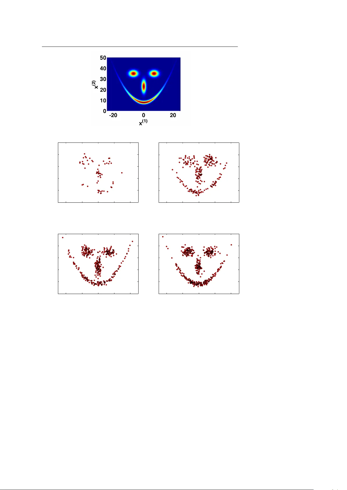
Noname man uscript No. (will b e inserted b y the editor) On the flexibilit y of the design of Multiple T ry Metrop olis sc hemes Luca Martino · Jesse Read Received: date / Accepted: date Abstract The Multiple T ry Metrop olis (MTM) metho d is a generalization of the classical Metrop olis-Hastings algorithm in whic h the next state of the c hain is c hosen among a set of samples, according to normalized weigh ts. In the literature, sev eral extensions ha v e been proposed. In this work, we show and remark up on the flexibility of the design of MTM-t yp e metho ds, fulfilling the detailed balance condition. W e discuss several p ossibilities and sho w different n umerical results. Keyw ords Metrop olis-Hasting metho d; Multiple T ry Metropolis algorithm; Multi-p oin t Metrop olis algorithm; MCMC techniques 1 Introduction Mon te Carlo metho ds are v ery useful to ols for scien tific and appro ximate computing, n umerical inference and optimization [6, 25]. F or instance, Mon te Carlo methods are often necessary for the implemen tation of optimal Ba y esian estimators so that several families of tec hniques hav e b een prop osed [7, 10]. The core of the Monte Carlo approach consists of drawing random samples from a target probabilit y density function (p df ). A very pow erful class of Monte Carlo techniques is the so-called Marko v Chain Mon te Carlo (MCMC) algorithms [9, 10, 15, 16, 25]. They generate a Mark ov c hain such that its stationary distribution coincides with the target probabilit y density function (pdf ). T ypically , the only requirement is to b e able to ev aluate the target function, where the kno wledge of the normalizing constan t is usually not needed. Luca Martino · Jesse Read Department of Signal Theory and Communications, Universidad Carlos I I I de Madrid T el.: 0034-916249192 E-mail: luca@tsc.uc3m.es, jesse@tsc.uc3m.es 2 Luca Martino, Jesse Read The most p opular MCMC metho d is undoubtedly the Metrop olis-Hasting (MH) algorithm [13, 20]. It can b e applied to almost an y arbitrary target distribution. How ev er, to sp eed up the con vergence and reduce the “burn- in” p erio d, sev eral extensions ha ve b een proposed in literature. F or instance, the Multiple T ry Metropolis (MTM) scheme [17] where, according to certain w eights, the next state of the Marko v chain is selected from a set of indep enden t samples drawn from a generic prop osal densit y . The main adv an tage of MTM is that it can explore a larger p ortion of the sample space without a decrease of the acceptance rate. Previously , a similar metho dology w as prop osed in the domain of molecular simulation, called “orien tational bias Mon te Carlo” [8, Chapter 13], where i.i.d. candidates are drawn from a symmetric proposal p df and one of these is chosen according to normalized w eights directly prop ortional to the target p df. Due to its goo d p erformance and the attractiv e possibility to com bine it with adaptive MCMC strategies [15, Chapter 8], [12] (for instance using differen t in teracting or adaptive prop osals at the same iteration [4]), the basic form ulation of the MTM has b een mo dified and stressed in different wa ys. In [22], the transition rule of the MTM algorithm is generalized such that the analytic form of the w eights is not specified. They also study the extension of the MTM in the rev ersible jump framew ork. In [4] an MTM scheme with differen t prop osal is introduced. Different approaches with correlated candidates hav e b een suggested in [5, 18, 24]. Some in teresting theoretical results on the asymptotic b ehavior of different MTM strategies and some considerations on the c hoice of the weigh ts are given in [2]. In all the proposed MTM schemes the n um ber of generated candidates is fixed, differently from the delay ed rejection Metrop olis algorithm [21, 30], and the state space is not augmented defining an extended target distribution, as in other MCMC metho ds based on auxiliary random v ariables [28]. In this work, we stress and remark upon the flexibilit y in the c hoice of transition rules within MTM algorithms. First of all, w e mix the approac hes from [4] and [22], building a MTM with generic weigh ts using different prop osal p dfs. Then, we presen t a general framework for the construction of acceptance probabilities in MTM schemes. W e sho w this theoretically and illustrate with sp ecific examples. Owing to this flexibility , it is also p ossible to design a MTM sc heme without drawing reference p oin ts [26]. Moreov er, we also in tro duce this kind of MTM algorithm with a determinist reference p oints, and then discuss ho w this c hange affects its performance. W e show that all the presen ted schemes fulfill the detailed balance condition and provide n umerical comparisons. Related considerations can b e found in [1, 3, 13, 23, 28, 29, 31]. The rest of the pap er is organized as follo ws. In Section 2 we combine the schemes in [4, 22] describing an MTM algorithm using different prop osal densities and generic weigh t functions. In Section 3, w e explain the flexibility in the c hoice of the acceptance functions, satisfying the detailed balance condition. Some examples of acceptance rules are shown in Section 4. Section 5 in tro duces a MTM metho d without generating the reference p oints randomly . On the flexibility of the design of Multiple T ry Metropolis sc hemes 3 Numerical comparisons are giv en in Section 6 and finally we draw conclusions in Section 7. 2 MTM algorithm with generic weigh ts and differen t proposals In the classical MH algorithm, a new possible state is drawn from the prop osal p df and the mov emen t is accepted with a decision rule that guarantees fulfillmen t of the balance condition. In a m ultiple try approach, sev eral (indep enden t [17, 22] or correlated [18, 24]) samples are generated and from these a “go o d” one is c hosen. In [4] the standard MTM is generalized using differen t proposal densities whereas in [22] the authors extend the standard MTM considering generic w eight functions. In the following section, w e recall and mix together b oth approac hes [4, 22] providing an extended MTM algorithm dra wing candidates from with different prop osals where the weigh t functions are not defined sp ecifically , i.e., the analytic form can b e chosen arbitrarily (they m ust b e b ounded and p ositiv e functions). 2.1 Algorithm Let p o ( x ) b e the p df that we wan t to draw from and p ( x ) a function prop ortional to our target pdf p o ( x ) (i.e., p ( x ) ∝ p o ( x )). Giv en a current state of the chain x t = x ∈ D ⊆ R , t ∈ N , (we assume scalar v alues only for simplicit y in the treatment), we dra w N independent samples each step from differen t prop osal p dfs, i.e., y 1 ∼ π 1 ( ·| x ) , y 2 ∼ π 2 ( ·| x ) , . . . , y N ∼ π N ( ·| x ) . Therefore, w e can write the joint distribution of the generated samples as q N ( y 1: N | x ) = π 1 ( y 1 | x ) π 2 ( y 2 | x ) · · · π N ( y N | x ) . Then, a “go o d” candidate among the generated samples is chosen according to w eight functions ω ( z 1 , z 2 ) ∈ R 2 → R + (where z 1 and z 2 are generic v ariables) that ha v e to be (a) b ounded and (b) positive. Given a curren t state x t = x , the algorithm can b e describ ed as follo ws: 1. Dra w N samples y 1: N = [ y 1 , y 2 , ..., y N ] from the join t p df q ( y 1: N | x ) = π 1 ( y 1 | x ) π 2 ( y 2 | x ) π 2 ( y 3 | x ) · · · π N ( y N | x ) , namely , dra w y j from π j ( ·| x ), with j = 1 , ..., N . 2. Calculate the weigh ts ω j ( y j , x ), j = 1 , ..., N , and normalize them to obtain ¯ ω j , j = 1 , ..., N . 4 Luca Martino, Jesse Read 3. Dra w a y = y k ∈ { y 1 , ...., y N } according to ¯ ω j , j = 1 , ..., N and set (recall that y k = y ) W y = ¯ ω k = ω k ( y , x ) P N j =1 ω j ( y j , x ) . (1) 4. Dra w other auxiliary samples (often called r efer enc e p oints ), x ∗ i ∼ π i ( ·| y ) for i = 1 , ..., k − 1 , k + 1 , ...., N , and set x ∗ k = x . 5. Compute the corresp onding w eigh ts ω j ( x ∗ j , y ), j = 1 , ..., N and set (recall that x ∗ k = x ) W x = ω k ( x, y ) P N j =1 ω j ( x ∗ j , y ) . (2) 6. Let x t +1 = y (recall that y = y k ) with probabilit y α ( x, y ) = min  1 , p ( y ) π k ( x | y ) p ( x ) π k ( y | x ) W x W y  , (3) otherwise set x t +1 = x with the remaining probabilit y 1 − α ( x, y ). 7. Set t = t + 1 and go back to the step 1. The k ernel of the algorithm abov e satisfies the detailed balance condition. The pro of is a sp ecial case of the developmen t that w e will present in Section 3.2, using the probabilit y α ( x, y ) in Eq. (3). 2.2 Sp ecial case: standard MTM algorithm Cho osing the w eight functions with the sp ecific analytic form ω i ( y i , x ) = p ( y i ) π i ( x | y i ) λ i ( x, y i ) , (4) with λ i ( x, y i ) = λ i ( y i , x ), i = 1 , ..., N , w e obtain the MTM sc heme proposed in [4] (with different prop osals). Indeed, note that the acceptance function (3) can b e also expressed as α ( x, y ) = min " 1 , p ( y ) π k ( x | y ) p ( x ) π k ( y | x ) ω k ( x, y ) ω k ( y , x ) P N j =1 ω j ( y j , x ) P N j =1 ω j ( x ∗ j , y ) # , and using the w eight choice in Eq. (4) , α ( x, y ) = min " 1 , p ( y ) π k ( x | y ) p ( x ) π k ( y | x ) p ( x ) π k ( y | x ) λ k ( x, y ) p ( y ) π k ( x | y ) λ k ( y , x ) P N j =1 ω j ( y j , x ) P N j =1 ω j ( x ∗ j , y ) # , then it is simplified α ( x, y ) = min " 1 , P N j =1 ω j ( y j , x ) P N j =1 ω j ( x ∗ j , y ) # . On the flexibility of the design of Multiple T ry Metrop olis schemes 5 Finally , observ e that if w e use just one proposal, π 1 ( y | x ) = π 2 ( y | x ) = ... = π N ( y | x ) and the same functions λ 1 ( x, y ) = λ 2 ( x, y ) = ... = λ N ( x, y ), w e obtain the standard form ulation of the MTM [17]. Figure 1 represents a general sc heme of the algorithm describ ed in Section 2.1. π 1 ( y 1 | x ) y 1 y N y 2 π 2 ( y 2 | x ) π N ( y N | x ) …. y = y k ω 1 ( y 1 ,x ) ω 2 ( y 2 ,x ) ω N ( y N ,x ) x ∗ i ∼ π i ( x ∗ i | y ) , i � = k, x ∗ k = x x = x t x t +1 Reference points α ( x, y )=m i n  p ( y ) π k ( x | y ) p ( x ) π k ( y | x ) W x W y  Fig. 1 Sk etch of the MTM algorithm with generic w eigh ts and differen t proposals described in Section 2.1. 2.3 Imp ortan t observ ations It is imp ortant to remark that, in order to obtain a fair comparison among the generated candidates, in the computation of the weigh ts, it is advisable to use prop osal functions with the same area b elow, i.e., R D π 1 ( y 1 | x ) dy 1 = R D π 2 ( y 2 | x ) dy 2 = ... = R D π N ( y N | x ) dy N , for instance they can b e normalized. This is not strictly needed but recommendable. Moreo ver, it is p ossible to show (see Section 3.2) that the algorithm ab ov e w orks owing to α ( x, y ) satisfies the following equation p ( x ) π k ( y | x ) W y α ( x, y ) = p ( y ) π k ( x | y ) W x α ( y , x ) . (5) Note that 0 ≤ W y ≤ 1 and 0 ≤ W x ≤ 1 are probabilities and functions of x , y , the remaining p oints y i and x ∗ i , then a more appropriate notation would b e W y ( y 1 , ..., y k = y , ..., y N , x ) and W x ( x ∗ 1 , ...x ∗ k = x, ..., x ∗ N , y ). 1 Ho wev er, for 1 Recall that y i are drawn from π i ( ·| x ) whereas x ∗ i are drawn from π i ( ·| y ), i = 1 , ..., N . 6 Luca Martino, Jesse Read simplicit y we main tain the notation W y and W x . In the sequel, we suggest differen t acceptance functions α ( x, y ). 3 Flexibility of the acceptance function Here, we introduce different multiple try MH approac hes with generic weigh ts functions. Sp ecifically w e show ho w to design different suitable acceptance functions α ( x, y ) fulfilling the detailed balance condition. Indeed, it is p ossible to c ho ose functions α ( x, y ) with the form α ( x, y ) = β ( x, y ) γ ( x, y | x ∗ − k , y − k ) , where 1. β ( x, y ) is such that p ( x ) π k ( y | x ) β ( x, y ) = p ( y ) π k ( x | y ) β ( y , x ) , ∀ k ∈ { 1 , ..., N } , (6) 2. γ ( x, y | x ∗ − k , y − k ) satisfies W y γ ( x, y | x ∗ − k , y − k ) = W x γ ( y , x | y − k , x ∗ − k ) , (7) where x ∗ − k = [ x ∗ 1 , ...x ∗ k − 1 , x ∗ k +1 , ..., x ∗ N ] and y − k = [ y 1 , ...y k − 1 , y k +1 , ..., y N ]. 3. Finally w e need 0 ≤ α ( x, y ) ≤ 1 . (8) If the Eqs. (6) and (7) are jointly fulfilled then the condition (5) also holds, i.e., the equation p ( x ) π k ( y | x ) W y α ( x, y ) = p ( y ) π k ( x | y ) W x α ( y , x ) is satisfied. Equation (8) can b e easily obtained choosing separately 0 ≤ β ( x, y ) ≤ 1 and 0 ≤ γ ( x, y | x ∗ − k , y − k ) ≤ 1. Moreov er, in this case, Eq. (6) is exactly the balance condition of the standard MH algorithm, then we can c ho ose an y acceptance functions suitable for the standard MH algorithm as function β ( x, y ). Similar considerations can b e used to design suitable functions γ ( x, y | x ∗ − k , y − k ). Some examples are pro vided in Section 4. 3.1 Algorithm The no vel sc heme can b e summarized as follows: 1. Dra w N samples from the prop osal p dfs y j ∼ π j ( ·| x ), with j = 1 , ..., N . 2. Calculate the weigh ts ω j ( y j , x ), j = 1 , ..., N , and normalize them to obtain ¯ ω j , j = 1 , ..., N . 3. Dra w a y = y k ∈ { y 1 , ...., y N } according to ¯ ω j , j = 1 , ..., N and set (recall that y k = y ) W y = ¯ ω k = ω k ( y , x ) P N j =1 ω j ( y j , x ) . On the flexibility of the design of Multiple T ry Metrop olis schemes 7 4. Dra w other auxiliary samples x ∗ i ∼ π i ( ·| y ) for i = 1 , ..., k − 1 , k + 1 , ..., N , and set x ∗ k = x . 5. Compute the corresp onding w eigh ts ω j ( x ∗ j , y ), j = 1 , ..., N and set (recall that x ∗ k = x ) W x = ω k ( x, y ) P N j =1 ω j ( x ∗ j , y ) . 6. Let x t +1 = y (recall that y = y k ) with probabilit y α ( x, y ) = β ( x, y ) γ ( x, y | x ∗ − k , y − k ) , where p ( x ) π k ( y | x ) β ( x, y ) = p ( y ) π k ( x | y ) β ( y , x ) and W y γ ( x, y | x ∗ − k , y − k ) = W x γ ( y , x | y − k , x ∗ − k ) . Otherwise set x t +1 = x with the remaining probabilit y 1 − α ( x, y ). 7. Set t = t + 1 and go back to the step 1. 3.2 Balance condition T o guaran tee that a Marko v chain generated by an MCMC metho d conv erges to the target distribution p o ( x ) ∝ p ( x ), w e can prov e that the k ernel A ( y | x ) of the corresp onding algorithm (probability of accepting a generated sample y giv en the previous state v alue x ) fulfills the following detailed balance condition 2 [16, 25] p ( x ) A ( y | x ) = p ( y ) A ( x | y ) . First of all, w e need to write down the kernel A ( y | x ). W e consider x 6 = y , since the case x = y is trivial (indeed, in this case A ( y | x ) is prop ortional to a delta function δ ( y − x ) [16, 25]). The kernel (for x 6 = y ) can b e expressed as A ( y = y k | x ) = N X i =1 h ( y = y k | x, k = i ) , where h ( y = y k | x, k = i ) is the probability of accepting the new state x t +1 = y k giv en the previous one x t = x , when the chosen sample y k is the i -th candidate, i.e., when y k = y i . Ho w ev er, since the y i are exc hangeable, for symmetry we ha ve h ( y = y k | x, i ) = h ( y = y k | x, j ) ∀ i, j ∈ { 1 , ..., N } . Hence, we can also write A ( y = y k | x ) = N · h ( y = y k | x, k ) , 2 Note that the balance condition is a sufficient but not necessary condition. Namely , the detailed balance ensures inv ariance. The conv erse is not true. Marko v chains that satisfy the detailed balance condition are called r eversible . 8 Luca Martino, Jesse Read where k ∈ { 1 , ..., N } and we recall N is the total n um b er of prop osed candidates y i . Then, w e need to show that p ( x ) h ( y | x, k ) = p ( y ) h ( x | y , k ) , for a generic k ∈ { 1 , ..., N } . F ollowing eac h step of the algorithm ab ov e, we can write p ( x ) h ( y = y k | x, k ) = p ( x ) Z D · · · Z D   N Y j =1 π j ( y j | x )   ω k ( y , x ) P N i =1 ω i ( y i , x )   N Y j =1; j 6 = k π j ( x ∗ j | y )   · β ( x, y ) γ ( x, y | x ∗ − k , y − k ) | {z } α ( x,y ) dy 1: k − 1 dy k +1: N dx ∗ 1: k − 1 dx ∗ k +1: N . Note that each factor inside the integral corresp onds to a step of the metho d describ ed in the previous section. The integral is ov er all auxiliary v ariables. Since we consider y = y k and recalling the definition of W y in Eq. (1), we can rewrite the expression in this w ay p ( x ) h ( y | x, k ) = p ( x ) Z D · · · Z D π k ( y | x )   N Y j =1 ,j 6 = k π j ( y j | x )   W y   N Y j =1; j 6 = k π j ( x ∗ j | y )   · · β ( x, y ) γ ( x, y | x ∗ − k , y − k ) dy 1: k − 1 dy k +1: N dx ∗ 1: k − 1 dx ∗ k +1: N . and w e only arrange it, obtaining p ( x ) h ( y | x, k ) = Z D · · · Z D   N Y j =1 ,j 6 = k π j ( y j | x )     N Y j =1; j 6 = k π j ( x ∗ j | y )   · · p ( x ) π k ( y | x ) β ( x, y ) · W y γ ( x, y | x ∗ − k , y − k ) d y − k d x ∗ − k . (9) Therefore, since w e assume (see Eqs. (6) and (7)) p ( x ) π k ( y | x ) β ( x, y ) = p ( y ) π k ( x | y ) β ( y , x ) , and W y γ ( x, y | x ∗ − k , y − k ) = W x γ ( y , x | y − k , x ∗ − k ) , it is straightforw ard that the expression in Eq. (9) is symmetric in x and y . Indeed, we can exc hange the notations of x and y , and x ∗ i and y j , resp ectively , and the expression do es not v ary . Then we can write p ( x ) h ( y | x, k ) = p ( y ) h ( x | y , k ) . On the flexibility of the design of Multiple T ry Metrop olis schemes 9 Since we hav e assumed a generic k and A ( y = y k | x ) = h ( y = y k | x, k ), it p ossible to assert that p ( x ) A ( y | x ) = p ( y ) A ( x | y ) , that is the balance condition. Therefore, the Marko v c hain generated by the algorithm, describ ed in the previous section, con verges to our target p df. 4 Examples of functions α ( x, y ) In this section, we provide some suitable acceptance functions α ( x, y ) = D × D → [0 , 1], that satisfies the condition (5). The easiest wa y is to obtain α ( x, y ) is to design separately suitable functions 0 ≤ β ( x, y ) ≤ 1 and 0 ≤ γ ( x, y | x ∗ − k , y − k ) ≤ 1. 4.1 P ossible choices of β ( x, y ) T o design a function β ( x, y ) such that 0 ≤ β ( x, y ) ≤ 1 and p ( x ) π k ( y | x ) β ( x, y ) = p ( y ) π k ( x | y ) β ( y , x ) , w e can choose any acceptance rule suitable for the standard MH algorithm [1, 13]. Hence, for instance, we can choose the classical acceptance rule of the MH algorithm, i.e., β 1 ( x, y ) = min  1 , p ( y ) π k ( x | y ) p ( x ) π k ( y | x )  . (10) Other p ossibilities are summarized in T able 1 where λ ( x, y ) is a symmetric non- negativ e function (i.e., λ ( x, y ) ≥ 0 and λ ( x, y ) = λ ( y , x ) for all ( x, y ) ∈ D × D ) suc h that 0 ≤ β ( x, y ) ≤ 1. T able 1 Example of suitable functions β ( x, y ) F unctions β ( x, y ) References β 1 ( x, y ) = min h 1 , p ( y ) π k ( x | y ) p ( x ) π k ( y | x ) i [13, 20] β 2 ( x, y ) = p ( y ) π k ( x | y ) p ( x ) π k ( y | x )+ p ( y ) π k ( x | y ) [1] β 3 ( x, y ) = λ ( x,y ) 1+ p ( x ) π k ( y | x ) p ( y ) π k ( x | y ) [13] β 4 ( x, y ) = p ( y ) π k ( x | y ) λ ( x,y ) [16, 25] β 5 ( x, y ) = λ ( x,y ) p ( x ) π k ( y | x ) [16, 25] β 6 ( x, y ) = p ( y ) λ ( x,y ) π k ( y | x ) [16, Chapter 5] β 7 ( x, y ) = π k ( x | y ) λ ( x,y ) p ( x ) [16, Chapter 5] 10 Luca Martino, Jesse Read Moreo ver, defining R ( x, y ) = p ( y ) π k ( x | y ) p ( x ) π k ( y | x ) , and considering a function F ( ϑ ) : R + → [0 , 1] suc h that F ( ϑ ) = ϑF (1 /ϑ ) , then it is p ossible to define a general acceptance function [9, 10] β g ( x, y ) = ( F ◦ R )( x, y ) = F ( R ( x, y )) . F or instance, if F ( ϑ ) = min[1 , ϑ ] w e obtain Eq. (10) and if F ( ϑ ) = ϑ 1+ ϑ w e find β 2 or β 3 with λ ( x, y ) = 1 (see T able 1). In [23] there is a comparison of differen t acceptance functions in a standard MH algorithm. 4.2 P ossible choices of γ ( x, y | x ∗ − k , y − k ) In this section, w e pro vide some examples of suitable function γ ( x, y | x ∗ − k , y − k ). W e need functions γ ( x, y | x ∗ − k , y − k ) suc h that W y γ ( x, y | x ∗ − k , y − k ) = W x γ ( y , x | y − k , x ∗ − k ) , (11) where W y = ω k ( y , x ) P N j =1 ω j ( y j , x ) , and W x = ω k ( x, y ) P N j =1 ω j ( x ∗ j , y ) . Therefore, for instance, it is p ossible to c ho ose γ 1 ( x, y | x ∗ − k , y − k ) = W x . Indeed, in this case γ ( y , x | y − k , x ∗ − k ) = W y and the condition (11) is satisfied ( W y W x = W x W y ). Another p ossibilit y is to define γ 2 ( x, y | x ∗ − k , y − k ) = W x W x + W y , or γ 3 ( x, y | x ∗ − k , y − k ) = min  1 , W x W y  . On the flexibility of the design of Multiple T ry Metrop olis schemes 11 5 MTM without drawing reference points The previous considerations also suggest ho w it is p ossible to design a MTM that av oids sampling the reference p oints x ∗ − k . F or some authors generating the reference samples is considered a dra wbac k of the MTM sc hemes, since N − 1 samples are only drawn to fulfill the balance condition [26]. T o av oid this step, the MTM metho d in Section 2.1 can b e mo dified as follows: 1. Giv en a current state x t = x , dra w N samples y 1: N = [ y 1 , y 2 , ..., y N ] from the join t p df q ( y 1: N | x ) = π 1 ( y 1 | x ) π 2 ( y 2 | x ) π 2 ( y 3 | x ) · · · π N ( y N | x ) , namely , dra w y j from π j ( ·| x ), with j = 1 , ..., N . 2. Calculate the weigh ts ω j ( y j , x ), j = 1 , ..., N , and normalize them to obtain ¯ ω j , j = 1 , ..., N . 3. Dra w a y = y k ∈ { y 1 , ...., y N } according to ¯ ω j , j = 1 , ..., N and set W y = ¯ ω k = ω k ( y , x ) P N j =1 ω j ( y j , x ) . (12) 4. Set x ∗ i = y i for i = 1 , ..., k − 1 , k + 1 , ...., N , and set x ∗ k = x . 5. Compute the corresp onding weigh ts ω j ( x ∗ j , y ), j = 1 , ..., N and (recalling x k ∗ = x ) set W x = ω k ( x, y ) P N j =1 ω j ( x ∗ j , y ) . (13) 6. Let x t +1 = y (recall that y = y k ) with probabilit y α ( x, y ) = min " 1 , p ( y ) Q N i =1 π i ( x ∗ i | y ) p ( x ) Q N i =1 π i ( y i | x ) W x W y # , (14) otherwise set x t +1 = x with the remaining probabilit y 1 − α ( x, y ). 7. Set t = t + 1 and go back to the step 1. The differences w.r.t. the standard MTM method are contained in the steps 4 and 6. In this case the v ectors y = [ y 1 , ..., y k = y, ...., y N ] and x ∗ = [ x ∗ 1 = y 1 , ..., x ∗ k = x, ...., x ∗ N = y N ] differ only in the p osition k , i.e., y − k = x ∗ − k . Hence, note that α ( x, y ) can b e expressed as α ( x, y ) = min " 1 , p ( y ) π k ( x | y ) p ( x ) π k ( y | x ) Q N i 6 = k π i ( y i | y ) Q N i 6 = k π i ( y i | x ) W x W y # . (15) Ho wev er, although this scheme satisfies the balance condition as we sho w b elo w, observing the expression of α , a dra wback could seem evident: since the samples y 1: N are drawn from π i ( ·| x ), i = 1 , .., N , the pro duct Q N i 6 = k π i ( y i | x ) w ould b e “often” greater then Q N i 6 = k π i ( y i | y ). That is to sa y , x is more “likely” than y given the “observ ations” y i , i 6 = k . Therefore, α ( x, y ) would b e “often” 12 Luca Martino, Jesse Read less than 1 so that accepting a jump becomes “rare” 3 . This issue w ould increase with N → + ∞ . How ev er, the numerical simulations (see Section 6) sho w that the probability α ( x, y ) first surprisingly increases for small v alues of N (owing to the factor W x W y ) and then decreases with N → + ∞ as exp ected. Moreo v er the p erformance generally gets worse with N → + ∞ . Hence this scheme app ears, in general, useless. These considerations ab ov e explain as, in the standard MTM version [17], the authors introduce the idea of randomly generating the reference p oints x ∗ i . How ev er, there is an imp ortant sp ecial case that we show in Section 5.2. 5.1 Balance condition Again w e m ust c hec k that the detailed balance condition p ( x ) A ( y | x ) = p ( y ) A ( x | y ) is fulfilled. The kernel A ( y | x ) (for x 6 = y ) can b e expressed, also in this case, as A ( y = y k | x ) = N · h ( y = y k | x, k ), where k ∈ { 1 , ..., N } and N is the total num b er of proposed candidates y i . Then, finally we hav e to show that p ( x ) h ( y | x, k ) = p ( y ) h ( x | y , k ) , for a generic k ∈ { 1 , ..., N } . F ollowing each step of the MTM algorithm without reference p oin t, we can write p ( x ) h ( y | x, k ) = p ( x ) Z D · · · Z D " N Y i =1 π i ( y i | x ) # W y min " 1 , p ( y ) Q N i =1 π i ( x ∗ i | y ) p ( x ) Q N i =1 π i ( y i | x ) W x W y # dy 1: k − 1 dy k +1: N dx ∗ 1: k − 1 dx ∗ k +1: N . The in tegral is ov er all auxiliary v ariables. Just by rearranging, we obtain p ( x ) h ( y | x, k ) = Z D · · · Z D min " p ( x ) N Y i =1 π i ( y i | x ) W y , p ( y ) N Y i =1 π i ( x ∗ i | y ) W x # dy 1: k − 1 dy k +1: N dx ∗ 1: k − 1 dx ∗ k +1: N . (16) Recalling that x ∗ j = y j for j = 1 , .., k − 1 , k + 1 , .., N , x ∗ k = x and y k = y , the Eq. (16) can b e rewritten as p ( x ) h ( y | x, k ) = Z D · · · Z D min   p ( x ) π k ( y | x ) N Y i 6 = k π i ( y i | x ) W y , p ( y ) π k ( x | y ) N Y i 6 = k π i ( y i | y ) W x   dy 1: k − 1 dy k +1: N . Therefore it is straightforw ard to see that we can exchange x and y without v arying the expression ab ov e (see also Eq. (12) and (13)), then p ( x ) h ( y | x, k ) = p ( y ) h ( x | y , k ) and the balance condition p ( x ) A ( y | x ) = p ( y ) A ( x | y ) is satisfied. 3 How ev er, it is imp ortant to remark that high acceptance rates are not a suitable indicator of go od performance since, in general, the b est acceptance rate is different from 1 [27]. On the flexibility of the design of Multiple T ry Metrop olis schemes 13 5.2 Indep enden t prop osal p dfs If the prop osal p dfs are chosen as indep endent densities, i.e., π 1 ( y 1 | x ) = π 1 ( y 1 ), π 2 ( y 2 | x ) = π 2 ( y 2 )... π N ( y N | x ) = π N ( y N ), the algorithm is simplified. Indeed, the α ( x, y ) probability in Eq. (15), i.e., α ( x, y ) = min " 1 , p ( y ) π k ( x | y ) p ( x ) π k ( y | x ) Q N i 6 = k π i ( y i | y ) Q N i 6 = k π i ( y i | x ) W x W y # , no w it can b e rewritten as α ( x, y ) = min " 1 , p ( y ) π k ( x ) Q N i 6 = k π i ( y i ) p ( x ) π k ( y ) Q N i 6 = k π i ( y i ) W x W y # = min  1 , p ( y ) π k ( x ) p ( x ) π k ( y ) W x W y  . Observ e that it is exactly the probabilit y α ( x, y ) obtained in Eq. (3) using indep enden t prop osals. Therefore, here, the conclusion is different from the general case: it is not necessary to draw reference p oints when indep endent prop osal densities are used. It is necessary just to set deterministically x ∗ i = y i for i = 1 , ..., k − 1 , k + 1 , ...., N , and set x ∗ k = x . This sp ecial case, when the w eights are c hosen as in Section 2.2, is also discussed in [16, Chapter 5]. Figure 2 depicts the scheme of a MTM with generic w eigh ts and differen t indep enden t prop osal p dfs, whereas Figure 3 shows virtually the simplest MTM algorithms, using the same indep enden t prop osal to dra w the N candidates and imp ortance weigh ts (Fig. 3(a)) or weigh ts prop ortional to the target (Fig. 3(b)). 4 In this sp ecial cases, the analysis of the algorithm is also simpler. Indeed, for instance, consider the case in Fig. 3(a). The acceptance probabilit y can b e expressed as α ( x, y ) = min " 1 , ω ( y ) + P N i 6 = k ω ( y i ) ω ( x ) + P N i 6 = k ω ( y i ) # , where w ( y i ) = p ( y i ) π ( y i ) . Note that, in this case clearly α ( x, y ) → 1 as N → ∞ , since the c hosen candidate is “extremely goo d” using the importance sampling principle, when N → ∞ . 6 Numerical simulations In this section, we pro vide numerical results comparing differen t MTM approac hes: using random w alks or indep endent prop osal pdfs, with differen t w eight functions, without dra wing the reference p oin ts and using different acceptance functions. All the results hav e been av eraged o v er 2000 runs and they are obtained generating 5000 iterations of the Marko v c hain, with the exception of the last example where w e only draw 500 samples. 4 Another simple MTM scheme is the “orientational bias Monte Carlo” [8, Chapter 13]. In this case, the proposal pdf m ust b e symmetric, i.e., π ( y | x ) = π ( x | y ), and the w eights must b e prop ortional to the target, i.e., ω ( y i ) = p ( y i ), i = 1 , ..., N . 14 Luca Martino, Jesse Read y 1 y N y 2 …. y = y k ω 1 ( y 1 ,x ) ω 2 ( y 2 ,x ) ω N ( y N ,x ) π 1 ( y 1 ) π 2 ( y 2 ) π N ( y N ) x = x t +1 α ( x, y )=m i n  1 , p ( y ) π k ( x ) p ( x ) π k ( y ) W x W y  Fig. 2 Scheme of MTM algorithm with generic weigh ts and different indep endent proposal pdfs. y 1 y N y 2 …. y = y k x = x t +1 π ( y ) α ( x, y )=m i n  1 , ω ( y )+  N i � = k ω ( y i ) ω ( x )+  N i � = k ω ( y i )  ω ( y N )= p ( y N ) π ( y N ) ω ( y 1 )= p ( y 1 ) π ( y 1 ) ω ( y 2 )= p ( y 2 ) π ( y 2 ) (a) y 1 y N y 2 …. y = y k x = x t +1 π ( y ) α ( x, y )=m i n  1 , π ( x ) π ( y ) p ( y )+  N i � = k p ( y i ) p ( x )+  N i � = k p ( y i )  w ( y 1 )= p ( y 1 ) w ( y 2 )= p ( y 2 ) w ( y N )= p ( y N ) (b) Fig. 3 Sk etch of the simplest MTM schemes using just one indep endent prop osal density , (a) with imp ortance weigh ts and (b) weigh ts prop ortional to p ( x ). In these cases, clearly α ( x, y ) → 1 as N → ∞ . 6.1 Random w alk prop osal densities Let X ∈ R b e a random v ariable 5 with bimo dal p df p o ( x ) ∝ p ( x ) = exp  − ( x 2 − 4) 2 / 4  = exp  − x 4 − 8 x 2 + 16 4  . (17) 5 Note that, in this work, we have mainly considered scalar v ariables in order to simplify the treatmen t and the notation. All the considerations and algorithms contained in this w ork are also valid for m ulti-dimensional v ariables (see, for instance, the last numerical example in Section 6.6). On the flexibility of the design of Multiple T ry Metrop olis schemes 15 W e wan t to draw samples from p o ( x ) using differen t MTM sc hemes. W e generate tries from a Gaussian prop osal with v ariance σ 2 and the mean dep ends on the previous state x of the c hain, i.e., π ( y | x ) ∝ exp  − ( y − x ) 2 2 σ 2  . (18) W e apply MTM metho ds using the prop osal ab ov e, different num b er of candidates N = 1 , 2 , 5 , 100 , 1000 and different standard deviation σ = 2 , 10. Imp ortance w eigh ts ω ( y i , x ) = p ( y i ) π ( y i | x ) are used to select a go o d candidate. Observ e that an MTM with N = 1 is exactly a standard MH algorithm. W e also apply different MTM techniques without dra wing the reference p oin ts (denoted as “MTM-without”) describ ed in Section 5. T ables 2 and 3 summarize the numerical results in terms of av eraged probability of accepting a mo vemen t and linear correlation b etw een the state x t and x t +1 . T able 2 Numerical results (prop osal as random walk, σ = 2, using imp ortance weigh ts). T echnique Num b er of tries Acceptance rate Linear correlation standard MH N = 1 0.3002 0.9053 (MTM with N = 1) MTM-rw N = 2 0.4363 0.8397 MTM-rw N = 5 0.6046 0.6989 MTM-rw N = 100 0.8647 0.1892 MTM-rw N = 1000 0.9557 0.0513 MTM-without N = 2 0.4229 0.9160 MTM-without N = 5 0.5121 0.9568 MTM-without N = 100 0.1902 0.9978 MTM-without N = 1000 0.0036 0.9993 T able 3 Numerical results (prop osal as random walk, σ = 10, using imp ortance weigh ts). T echnique Num b er of tries Acceptance rate Linear correlation standard MH N = 1 0.0991 0.9085 (MTM with N = 1) MTM-rw N = 2 0.1795 0.8335 MTM-rw N = 5 0.3483 0.6700 MTM-rw N = 100 0.8373 0.1676 MTM-rw N = 1000 0.9483 0.0522 MTM-without N = 2 0.1810 0.8376 MTM-without N = 5 0.3575 0.7017 MTM-without N = 100 0.4453 0.9264 MTM-without N = 1000 0.2612 0.9952 It is important to remark that high acceptance rates are not a suitable indicator of go o d p erformance since, in general, the b est acceptance rate is 16 Luca Martino, Jesse Read differen t from 1 [27]. Therefore, b etter p erformance is indicated b y smaller correlations. W e show also the acceptance rates b ecause of the MTM metho d (dra wing the reference points) presents a b ehavior typical in adaptive MCMC algorithms where the adaptive prop osal p df con v ergence to the true shap e of the target [19]: the acceptance rate grows and the linear correlation decreases quic kly as N → + ∞ . Indeed, we can observe that, in b oth cases σ = 2 , 10, the correlation obtained with the MTM decreases to zero as N → + ∞ . Without dra wing the reference p oin ts, the resulting algorithm is totally useless for σ = 2 (T able 2) whereas it outp erforms the standard MH for N = 2 and N = 5 for σ = 10 (T able 3). How ev er, increasing N the performance gets worse. The results in T able 3 suggest that it exists an optimal n um b er of tries for an MTM sc heme without generating randomly the reference p oin ts. How ev er, the MTM metho d with the additional cost of the random generation of reference p oin ts alwa ys outperforms the general scheme describ ed in Section 5. With indep enden t prop osal p dfs this is not true as we show later. 6.2 Differen t choice of the weigh ts Considering the same target p df in Eq. (17), the Gaussian prop osal with σ = 10 in Eq. (18) (random w alk) and using N = 100 tries, we hav e compared the p erformance of differen t weigh t functions. T able 4 summarizes the results. T able 4 Numerical results (prop osal as random walk, σ = 10, N = 100 tries). W eights Acceptance rate Linear correlation ω i ( y i , x ) = p ( y i ) π i ( y i | x ) 0.8373 0.1676 importance weigh ts ω i ( y i , x ) = p ( y i ) 0.8374 0.1959 ω i ( y i , x ) = 1 0.0988 0.9090 ω i ( y i , x ) = p p ( y i ) 0.7036 0.3340 ω i ( y i , x ) = [ p ( y i )] 2 0.6870 0.3093 ω i ( y i , x ) = [ p ( y i )] 3 0.4476 0.4020 ω i ( y i , x ) = π i ( x | y i ) 0.1348 0.8809 ω i ( y i , x ) = 1 π i ( y i | x ) 0.0365 0.9652 ω i ( y i , x ) = p ( y i ) π i ( x | y i ) 0.8371 0.2248 The b est results are pro vided b y the importance w eigh ts ω i ( y i , x ) = p ( y i ) π i ( y i | x ) . The weigh ts of the form ω i ( y i , x ) = p ( y i ) and ω i ( y i , x ) = p ( y i ) π i ( x | y i ) also yield small correlation. Clearly , the c hoice ω i ( y i , x ) = 1 produces the same results of a standard MH since the selected candidate is chosen uniformly among the set of dra wn tries y i , i = 1 , ..., N , without using any information of the target or the prop osal functions. On the flexibility of the design of Multiple T ry Metrop olis schemes 17 6.3 Indep enden t prop osal densities In order to draw samples from the target in Eq. (17), we also apply MTM algorithms with indep enden t prop osal densities (MTM-ind) as π ( y ) ∝ exp  − ( y − µ ) 2 2 σ 2  , with σ = 10. In a first scheme, we generate N = 100 candidates from one proposal with µ = 0. Moreov er, in other scheme, we use tw o differen t indep enden t proposal pdfs with µ 1 = − 10 and µ 2 = 2. In this case, w e draw N / 2 = 50 tries from each one. W e apply these schemes with importance w eights, ω i ( y i , x ) = p ( y i ) π i ( y i ) , and also with w eights just prop ortional to the target p df, ω i ( y i , x ) = p ( y i ). T able 5 sho ws the numerical results. T able 5 Numerical results ( σ = 10, N = 100 tries). Prop osal p dfs Acceptance rate Linear correlation MTM-rw with 0.8373 0.1676 ω i ( y i , x ) = p ( y i ) π i ( y i | x ) MTM-rw with 0.8374 0.1959 ω i ( y i , x ) = p ( y i ) MTM-ind with 0.9760 0.0252 one prop osal p df ( µ = 0) and ω i ( y i , x ) = p ( y i ) π i ( y i | x ) MTM-ind with 0.9751 0.0267 one prop osal p df ( µ = 0) and ω i ( y i , x ) = p ( y i ) MTM-ind with 0.7420 0.2748 tw o prop osal p dfs ( µ 1 = − 10 and µ 2 = 2) and ω i ( y i , x ) = p ( y i ) π i ( y i | x ) MTM-ind with 0.7509 0.6622 tw o prop osal p dfs ( µ 1 = − 10 and µ 2 = 2) and ω i ( y i , x ) = p ( y i ) The first tw o lines of the T able 5 recall the acceptance rates and the linear correlations using the random walk proposal densities. The table sho ws that the MTM with independent proposal with µ = 0 provides the best results, i.e., the smallest correlation. How ev er, the results depend strongly on a suitable tuning of the parameter µ . Also in this case, the imp ortance w eights seem to provide b etter results. Another imp ortant consideration is that, using tw o prop osal p dfs, the MTM has selected a candidate generated from the prop osal with µ 1 = − 10 with a rate of 39 . 5% using imp ortance weigh ts, and just 1 . 5% with the w eights prop ortional to the target. This observ ation can b e extremely imp ortan t to design an adaptive strategy where the best prop osal density is c hosen among of a set of prop osals. 18 Luca Martino, Jesse Read 6.4 Hea vy tails In order to analyze the performance of the MTM schemes with hea vy tails, no w we consider as target p df the so-called L´ evy distribution for non-negative random v ariable, namely , p o ( x ) ∝ p ( x ) = 1 ( x − η ) 3 / 2 exp  − ν 2( x − η )  , ∀ x ≥ η ≥ 0 . (19) The normalizing constant 1 c p , such that p o ( x ) = 1 c p p ( x ), is analytically known, 1 c p = p ν 2 π . Moreov er, given a random v ariable X ∼ p o ( x ), all the momen ts E [ X γ ] with γ ≥ 1 do not exist owing to the heavy tail characteristic of the L ´ evy distribution. Our goal is to estimate the normalizing constant 1 c p via Monte Carlo sim ulation, when η = 0 and ν = 2, generating 5000 iterations of the Mark ov chain. W e apply three differen t MTM techniques with N = 1000 tries (drawing the reference p oints) and using imp ortance weigh ts to choose a suitable candidate eac h step. In the first t w o schemes (MTM-ind), w e use an indep enden t prop osal π ( x t ) ∝ exp {− ( x t − µ ) 2 / (2 σ 2 ) } with µ = 10 , 100 and σ = 50, whereas, in the last one (MTM-rw), w e use a random walk prop osal π ( x t | x t − 1 ) ∝ exp {− ( x t − x t − 1 ) 2 / (2 σ 2 ) } with σ = 50. W e c hoose huge v alues of σ due to the heavy tail feature of the target. W e ha ve av eraged all the results o ver 2000 runs and they are summarized in T able 6. The real v alue of 1 c p when ν = 2 is q 2 2 π = 0 . 5642. 6 T able 6 Estimation of the constant 1 c p = q 2 2 π = 0 . 5642 and standard deviation of the estimation ( N = 1000 tries). T echnique Estimation Std of F urther informations of 1 c p the estimation MTM-ind 0.6056 0.0012 µ = 10, σ = 50 MTM-ind 0.5994 0.0010 µ = 100, σ = 50 MTM-rw 0.5819 0.0050 σ = 50 6.5 Differen t acceptance probabilities In this section, we consider again the bimo dal target densit y in Eq. (17), i.e., p o ( x ) ∝ p ( x ) = exp  − ( x 2 − 4) 2 / 4  , and we generate candidates from a random walk Gaussian density with σ = 1, i.e., π ( y | x ) ∝ exp n − ( y − x ) 2 2 o . 6 W e do not provide the estimated linear correlation because of the momen ts (as the mean, for instance) of the target do not exist, and it makes difficult a right estimation of the correlation. On the flexibility of the design of Multiple T ry Metrop olis schemes 19 W e c ho ose as w eight functions ω ( x, y ) = [ p ( x )] θ , with θ = 1 / 2. Note that they cannot be obtained using the analytic form necessary in the standard MTM [17]. Moreov er, w e consider four p ossible com binations of the β ( x, y ) and γ ( x, y ) functions α 1 , 1 ( x, y ) = β 1 ( x, y ) γ 1 ( x, y ) , α 1 , 2 ( x, y ) = β 1 ( x, y ) γ 2 ( x, y ) , α 1 , 3 ( x, y ) = β 1 ( x, y ) γ 3 ( x, y ) , α 2 , 3 ( x, y ) = β 2 ( x, y ) γ 3 ( x, y ) , where each β i ( x, y ), i = 1 , 2, and γ j ( x, y ), j = 1 , 2 , 3, are defined in Sections 4.1 and 4.2. Then, we run the different MTM algorithms with N = 10 and N = 100 candidates. T able 7 sho ws the acceptance rate (the a v eraged probability of accepting a mov emen t) and normalized linear correlation co efficient (b etw een one state of the c hain and the next) a v eraged o v er 2000 runs and obtained with the differen t techniques where N = 10. T able 7 Numerical results with N = 10. F unction α Acceptance rate Linear correlation α 1 , 1 ( x, y ) 0.1167 0.9932 α 1 , 2 ( x, y ) 0.3246 0.9811 α 1 , 3 ( x, y ) 0.5512 0.9756 α 2 , 3 ( x, y ) 0.3370 0.9806 T able 8 illustrates the results using N = 100. W e observe that α 1 , 3 pro vides that greatest acceptance rate and lo west correlation in b oth cases. The acceptance rate of α 1 , 1 decreases with N = 100 because of γ 1 ( x, y | x ∗ − k , y − k ) = W x diminishes with the n umber of tries N . Moreov er, the correlation app ears (almost) in v arian t with the num ber of tries N . T able 8 Numerical results with N = 100. F unction α Acceptance rate Linear correlation α 1 , 1 ( x, y ) 0.0173 0.9931 α 1 , 2 ( x, y ) 0.3354 0.9828 α 1 , 3 ( x, y ) 0.5904 0.9737 α 2 , 3 ( x, y ) 0.3540 0.9859 Better p erformances can b e attained using the acceptance function of [22] and rewritten in Eq. (3), as exp ected analyzing the analytic form of the differen t acceptance functions. Indeed, w e obtain acceptance rates of 0 . 74, 0 . 81 and correlation 0 . 96, 0 . 96 with N = 10 and N = 100, resp ectively . 20 Luca Martino, Jesse Read 6.6 Smiling-F ace distribution In this section, we show that the p ow er of the MTM schemes increases when they draw from more complicated target distributions in higher dimensions, w.r.t. a standard MH algorithm. T o pro vide a graphical example, we consider a bidimensional target pdf p o ( x ) (where x = [ x (1) , x (2) ] T ∈ R 2 , x ( i ) ∈ R , i = 1 , 2) comp osed as a mixture of 4 densities, p o ( x ) ∝ 1 4 4 X i =1 p i ( x ) . (20) The first three comp onen ts are prop ortional to biv ariate Gaussian p dfs, i.e., p i ( x ) = p i ( x (1) , x (2) ) = exp      −  x (1) − µ (1) i  2 2  σ (1) i  2 −  x (2) − µ (2) i  2 2  σ (2) i  2      , with i = 1 , 2 , 3, µ (1) 1 = − 7, µ (2) 1 = 35, µ (1) 2 = 7, µ (2) 2 = 35, µ (1) 3 = 0 , µ (2) 3 = 23, σ (1) 1 = 2, σ (2) 1 = 2, σ (1) 2 = 2, σ (2) 2 = 2, σ (1) 3 = 1 and σ (2) 3 = 4. The last comp onen t is a banana-shap ed density [11, 14], i.e., p 4 ( x ) = p 4 ( x (1) , x (2) ) = exp      −  x (1)  2 η −  x (1) − ρ  x (2)  2 + 100 ρ  2 2      , with η = 144 . 5 and ρ = 0 . 08. The banana-shap ed distribution was first in tro duced in [11] and is known in literature to b e a difficult target. This kind of bidimensional and multimodal mixtures of densities is often used to compare the p erformance of differen t MCMC tec hniques [15, Chapter 5], [11, 12, 14]. The parameters of the Gaussian components and the banana-shap ed pdf are c hosen in order to form a “smiling face” as illustrated in Figure 4(a). The reason is that, in this w ay , it is p ossible to illustrate gr aphic al ly the p erformance of differen t samplers, as we show b elo w. T o draw from p o ( x ), we apply a MH and a MTM scheme using for b oth a random w alk Gaussian prop osal p df, i.e., π ( x t | x t − 1 ) ∝ exp  −  x (1) t − x (1) t − 1  2 / (2 σ 2 p ) −  x (2) t − x (2) t − 1  2 / (2 σ 2 p )  . In order to show the sp eed of the con vergence of the samplers, we hav e generated only 500 samples with a MTM with different num ber of candidates N = 1 , 5 , 100 , 1000 (note with N = 1 is a standard MH) and different standard deviation σ p = 5 , 10 of the prop osal. T ables 9-10 pro vide the a verage acceptance probabilit y of a new state in the first column (the av eraged v alues of α ), the jump rate among different modes in the second column (from “left ey e” to the “smile”, or from the “smile” to the “nose” etc.) and the linear correlation for each comp onent of x , in the On the flexibility of the design of Multiple T ry Metrop olis schemes 21 last column. T o compute the mo de-jump rate w e establish that the state x t b elongs to the mo de i ∗ if i ∗ = arg max i ∈{ 1 ,..., 4 } p i ( x t ) , where p i ( x t ) are the 4 comp onents in the mixture of Eq. (20). All results are a veraged o ver 2000 runs using σ p = 5 in T able 9 and σ p = 10 in T able 10. T able 9 Numerical results with σ p = 5. Num b er of tries N Acceptance Rate Mo de-Jump Rate Correlation N = 1 (standard MH) 0.2296 0.0401 x (1) → 0.9460 x (2) → 0.9749 N = 5 0.5118 0.1166 x (1) → 0.8661 x (2) → 0.9492 N = 100 0.7137 0.3373 x (1) → 0.6193 x (2) → 0.8508 N = 1000 0.7919 0.4430 x (1) → 0.4724 x (2) → 0.7662 T able 10 Numerical results with σ p = 10. Num b er of tries N Acceptance Rate Mo de-Jump Rate Correlation N = 1 (standard MH) 0.1464 0.0598 x (1) → 0.9097 x (2) → 0.9653 N = 5 0.4207 0.2313 x (1) → 0.7536 x (2) → 0.8454 N = 100 0.7670 0.5020 x (1) → 0.3570 x (2) → 0.4607 N = 1000 0.8930 0.6520 x (1) → 0.1635 x (2) → 0.1453 F rom the tables, we can observe that the MTM clearly outp erforms the standard MH since, as N gro ws, the correlation decreases and the mo de-jump rate increases (as does the acceptance rate) regardless of the chosen parameter σ p of the prop osal. Obviously , the mo de-jump rate is alwa ys less than the a verage v alue of the probability α of accepting a mo v emen t (the acceptance rate), since the mo de-jumps represen t a subset of all accepted mov emen ts. Moreo ver, the standard deviation σ p = 10 of the prop osal p df w orks b etter for the MTM metho d. In general, the MTM schemes w ork better with huge scaling parameters and a great-enough n um ber of candidates N (see also the discussion in the next section). Figures 4(b)-(c)-(d)-(e) depict generated samples ov er one run. Clearly , in general we observe less than 500 p oints since in certain cases a new mov emen t 22 Luca Martino, Jesse Read is rejected and the chain remains in the same state. Namely , certain points are rep eated. This effect is evident with the standard MH ( N = 1) whereas it v anishes as the num ber of candidates N grows. Moreo v er, with greater N , the n um b er of jumps among different mo des also increases quickly . As a consequence, with the MTM tec hnique ( N = 5 , 100 , 1000) all the features of the “face” (our target p df ) are completely describ ed since the con v ergence of the c hain is clearly sp eeded up. Therefore, with this numerical example, the main adv an tage of an MTM metho d b ecomes apparent: it can explore a larger p ortion of the sample space without a decrease of the acceptance rate, or even an increase thereof. 7 Discussion In this w ork, w e ha ve studied the flexibilit y in the design of MTM techniques. W e ha ve in troduced an MTM with generic weigh t functions (the analytic form can b e chosen arbitrarily) and different prop osal densities (each candidate can b e drawn from a different p df ) combining the algorithms in [4] and [22]. Moreov er, we hav e prop osed a general framework for construction of acceptance probabilities in the MTM sc hemes, providing also specific examples. Finally , w e hav e also designed a MTM algorithm without the need of generating randomly the reference p oints [26]. W e ha ve pro v ed that the nov el tec hniques satisfy the detailed balance condition, and carried out numerical sim ulations. Observing the theoretical workings and the numerical results, we can infer the follo wing conclusions and observ ations: 1. Gener al c onsider ations: The classical MTM metho d, prop osed in [17], clearly outp erforms the standard MH algorithm using the same proposal p df, in the sense that as the num ber of candidates increases, N → ∞ , then the correlation decreases quic kly to zero (see Section 6.3 for further considerations). If a designed MTM sc heme does not fulfill this property , then it is totally useless since the computational cost increased but the p erformance is not improv ed. Suitable MTM metho ds can b e applied efficien tly to an y kind of target distributions (bounded or unbounded, with hea vy tails or not), as shown in our n umerical simulations (see Section 6.4). Moreo ver, the adv an tages of using an MTM tec hnique w.r.t. a standard MH algorithm clearly gro w as the dimensionality of the target increases. 2. MTM schemes as black-b ox algorithms: the n umerical simulations show that, with a suitable n um ber of tries N , the MTM methods pro vide go o d results indep enden tly of the choice of the parameters of the prop osal. Therefore, it is imp ortant to remark that, ev en if no information ab out the target is a v ailable (for instance, ab out the location of the modes), an MTM sc heme allows the use of a prop osal p df with a huge scaling parameter in order to explore quic kly differen t regions of the space. Indeed, using a great-enough num b er of tries, this black-box approac h is quite robust and alw ays gives satisfactory p erformance. On other hand, with a h uge scaling On the flexibility of the design of Multiple T ry Metrop olis schemes 23 parameter, a standard MH usually pro duces a very small rate of jumps and, as a consequence, a v ery high correlation. 3. Choic e of the weights: the p ossibility to c hoose an y b ounded and p ositive w eight functions makes the MTM sc heme easier to be designed since the user should not chec k any conditions to use suitable weigh ts (as to chec k symmetry of the function λ , for instance) indep endently of the choice of the prop osal p dfs. Namely , the prop osal distribution and the weigh t functions can b e selected separately , to fit w ell to the sp ecific problem and to improv e the performance of the tec hnique. Note that, in some MTM approac hes the symmetry condition of the function λ can b e complicated, see for instance [18, 24]. F urther theoretical or numerical studies are needed to determine the b est c hoice of weigh t functions given a certain prop osal and target density . W e find that the w eights of the analytic form proposed in [17] (see for instance Eq. (4)) usually pro vide better results. Within this class, the imp ortance w eights ω i ( y i ) = p ( y i ) π i ( y i | x ) , based on the imp ortance sampling principle [16, 25], app ear to b e a goo d choice in theory . Numerical results also suggest that weigh ts simply prop ortional to the target densit y ω i ( y i ) = p ( y i ) can pro vide go o d p erformance. In [2] the authors note that imp ortance w eights place higher probabilit y on selecting candidates that are further a wa y from the curren t state of the chain, but finally they prefer to use w eights prop ortional to the target density based on n umerical results. If the ev aluation of the target p ( x ) is computationally exp ensive such that the target function can not b e included in the calculations of the weigh ts, then the w eigh t functions of the analytic class ω i ( y i , x ) = p ( y 1 ) π i ( x | y i ) λ ( x, y i ) prop osed in [17] cannot b e used. Indeed, it is imp ossible to find a symmetric function λ ( x, y ) = λ ( y , x ) in order to remo ve the dep endence on p ( x ) in the w eights (in this case there is just one p ossibilit y that p ( x ) is constant, i.e., p ( x ) = p ( y ) for all x, y ∈ D ). In this case, a p ossible c hoice of the weigh ts can be prop ortional to the proposal p dfs, namely w ( y i ) = π ( x | y i ) for instance. Clearly , it is not the optimal c hoice but, also in this case, the MTM can help to explore easily a larger p ortion of the sample space w.r.t. standard MH (see Section 6.2). 4. Use of differ ent pr op osal p dfs: a MTM scheme with different prop osal densities can be a v ery p ow erful framew ork mainly to tackle applications with high dimensionality and target distributions with several modes. In our opinion, the most promising scenario is to use different indep endent prop osal distributions up dating certain parameters (as mean and v ariance) eac h iteration of the c hain, or selecting the b est prop osal among a set of functions (see Section 6.3 for further considerations). In this adaptiv e framew ork, the indep endent prop osal p dfs could improv ed to fit better w.r.t. the target. This sc heme has not been already exploited completely . It is imp ortan t to remark that, in order to obtain a fair comparison among the generated candidates, it is recommendable to use proposal functions with the same area b elo w, for instance they can b e normalized. 24 Luca Martino, Jesse Read 5. Flexibility of the ac c eptanc e pr ob abilities: we hav e shown there are certain freedom degrees in the design of an MTM algorithm, sp ecifically in the c hoice of the acceptance probabilit y α . This is also confirmed by other w orks in literature that design suitable MTM schemes with correlated candidates but they are quite differen t (the strategies in [18, 24] generate the candidates sequentially , whereas the approac h in [5] uses a blo ck philosoph y). How ev er, although the detailed balance condition is alwa ys satisfied in all cases, the p erformance is differen t. Numerical results suggest that α functions as close as p ossible to the standard MTM method [17], using also the weigh ts of the analytic form in Eq. (4), p erform b etter results. Similar considerations can b e done ab out the standard MH algorithm [1, 13, 23]. 6. R efer enc e p oints: we hav e described a p ossible MTM algorithm without dra wing reference points. As seen in the numerical results, in this case it seems to exist an optimal v alue of the num ber of candidates N . As N → ∞ the p erformance b ecomes very p o or. Therefore, we can figure out that the “secret” of the goo d p erformance of the standard MTM scheme in [8, 17] is contained in the random generation of the reference p oin ts. Ho wev er, there exists an imp ortant sp ecial case where the reference p oin ts are completely unnecessary: using independent prop osal densities. In this case, the reference p oints can be set deterministically , equal to the previous generated candidates. This scheme, using just one prop osal (dra wing N candidates from the same p df ) jointly with importance weigh ts, app ears as the easiest and natural pro cedure to combine the classical MH algorithm and imp ortance sampling [25] (see Figure 3(a)). 7. Numb er of c andidates: All the schemes prop osed in literature and also in this work use a fixed n um b er of candidates N . An imp ortan t impro v ement w ould consist on tuning adaptiv ely the num ber N dep ending on the discrepancy b et ween target and prop osal distributions. T o do this, a certain measure is needed, for instance, as the effe ctive sample size of the imp ortance sampling framew ork [16, 25]. Clearly , this idea could be more effectiv e using indep enden t prop osal pdf since it is necessary to measure the discrepancy betw een the proposal and the target functions (with a random w alk, for instance, the mean of the prop osal changes each step and the distance w.r.t. the target v aries as well). Another p ossibility could b e to combine MTM and the delay ed rejection metho d [21, 30]. With this kind of pro cedures, the optimal trade off b etw een computational cost and p erformance w ould b e achiev ed. 8 Ackno wledgmen ts W e would like to thank the Reviewers for their commen ts which hav e help ed us to improv e the first version of manuscript. Moreov er, this work has b een partially supp orted by Ministerio de Ciencia e Innov acin of Spain (pro ject MONIN, ref. TEC-2006-13514-C02- 01/TCM, Program Consolider- On the flexibility of the design of Multiple T ry Metrop olis schemes 25 Ingenio 2010, ref. CSD2008- 00010 COMONSENS, and Distribuited Learning Comm unication and Information Pro cessing (DEIPR O) ref. TEC2009-14504- C02-01) and Comunidad Autonoma de Madrid (pro ject PROMUL TIDIS-CM, ref. S-0505/TIC/0233). References 1. A. A. Barker. Monte Carlo calculations of the radial distribution functions for a proton-electron plasma. A ustr alian Journal of Physics , 18:119–133, 1965. 2. M. B ´ edard, R. Douc, and E. Mouline. Scaling analysis of multiple-try MCMC metho ds. Sto chastic Pr o c esses and their Applic ations , 122:758– 786, 2012. 3. S. P . Bro oks. Marko v Chain Mon te Carlo metho d and its application. Journal of the R oyal Statistic al So ciety. Series D (The Statistician) , 47(1):69–100, 1998. 4. R. Casarin, R. V. Craiu, and F. Leisen. Interacting multiple try algorithms with different prop osal distributions. Statistics and Computing , pages 1– 16, Decem b er 2011. 5. R. V. Craiu and C. Lemieux. Acceleration of the Multiple-Try Metrop olis algorithm using antithetic and stratified sampling. Statistics and Computing , 17(2):109–120, 2007. 6. L. Devro ye. Non-Uniform R andom V ariate Gener ation . Springer, 1986. 7. W. J. Fitzgerald. Mark ov Chain Mon te Carlo methods with applications to signal pro cessing. Signal Pr o c essing , 81(1):3–18, January 2001. 8. D. F renkel and B. Smit. Understanding mole cular simulation: fr om algorithms to applic ations . Academic Press, San Diego, 1996. 9. D. Gamerman. Markov Chain Monte Carlo: Sto chastic Simulation for Bayesian Infer enc e . Chapman and Hall/CRC, 1997. 10. W.R. Gilks, S. Ric hardson, and D. Spiegelhalter. Markov Chain Monte Carlo in Pr actic e: Inter disciplinary Statistics . T a ylor & F rancis, Inc., UK, 1995. 11. H. Haario, E. Saksman, and J. T amminen. Adaptive proposal distribution for random walk Metrop olis algorithm. Computational Statistics , 14:375– 395, 1999. 12. H. Haario, E. Saksman, and J. T am minen. An adaptive Metrop olis algorithm. Bernoul li , 7(2):223–242, April 2001. 13. W. K. Hastings. Monte Carlo sampling metho ds using Marko v chains and their applications. Biometrika , 57(1):97–109, 1970. 14. S. Lan, V. Stathop oulosy , B. Shahbaba, and M. Girolami. Langrangian dynamical Mon te Carlo. , Nov ember 2012. 15. F. Liang, C. Liu, and R. Caroll. A dvanc e d Markov Chain Monte Carlo Metho ds: L e arning fr om Past Samples . Wiley Series in Computational Statistics, England, 2010. 16. J. S. Liu. Monte Carlo Str ate gies in Scientific Computing . Springer, 2004. 26 Luca Martino, Jesse Read 17. J. S. Liu, F. Liang, and W. H. W ong. The Multiple-Try metho d and lo cal optimization in Metrop olis sampling. Journal of the Americ an Statistic al Asso ciation , 95(449):121–134, March 2000. 18. L. Martino, Victor P ascual Del Olmo, and Jesse Read. A multi-point Metrop olis scheme with generic weigh t functions. Statistics & Pr ob ability L etters , 82(7):1445–1453, 2012. 19. L. Martino, J. Read, and D. Luengo. Impro ved adaptive rejection Metrop olis sampling algorithms. , 2012. 20. N. Metrop olis, A. Rosenbluth, M. Rosen bluth, A. T eller, and E. T eller. Equations of state calculations by fast computing mac hines. Journal of Chemic al Physics , 21:1087–1091, 1953. 21. A. Mira. On Metrop olis-Hastings algorithms with delay ed rejection. Metr on , 59:231–241, 2001. 22. Silvia Pandolfi, F rancesco Bartolucci, and Nial F riel. A generalization of the Multiple-try Metrop olis algorithm for Bay esian estimation and mo del selection. Journal of Machine L e arning R ese ar ch (Workshop and Confer enc e Pr o c e e dings V olume 9: AIST A TS 2010) , 9:581–588, 2010. 23. P .H. Peskun. Optim um Mon te-Carlo sampling using Mark o v chains. Biometrika , 60(3):607–612, 1973. 24. Z. S. Qin and J. S. Liu. Multi-Point Metrop olis metho d with application to h ybrid Monte Carlo. Journal of Computational Physics , 172:827–840, 2001. 25. C. P . Rob ert and G. Casella. Monte Carlo Statistic al Metho ds . Springer, 2004. 26. C.P . Rob ert. “Xi’ An’s Og, an attempt at bloggin... ” Blog (by Christian P. Rob ert). http://xianblo g.wor dpr ess.c om/2012/01/23/multiple-tryp oint- metr op olis-algorithm/ , January 2012. 27. G. O. Rob erts, A. Gelman, and W. R. Gilks. W eak conv ergence and optimal scaling of random walk Metrop olis algorithms. Annals of Applie d Pr ob ability , 7:110–120, 1997. 28. G. Storvik. On the flexibilit y of Metrop olis-Hastings acceptance probabilities in auxiliary v ariable prop osal generation. Sc andinavian Journal of Statistics , 38(2):342–358, F ebruary 2011. 29. L. Tierney . Marko v chains for exploring p osterior distributions. Ann. Statist. , 33:1701–1728, 1994. 30. L. Tierney and A. Mira. Some adaptiv e Mon te Carlo metho ds for Bay esian inference. Stat. Me d. , 18:2507–2515, 1999. 31. Y. Zhang and W. Zhang. Improv ed generic acceptance function for multi- p oin t Metrop olis algorithm. 2nd International Confer enc e on Ele ctr onic and Me chanic al Engine ering and Information T e chnolo gy (EMEIT-2012) , 2012. On the flexibility of the design of Multiple T ry Metrop olis schemes 27 (a) ï 20 ï 10 0 10 20 0 10 20 30 40 50 x (1) x (2) Standard MH ( N =1 ) (b) ï 20 ï 10 0 10 20 0 10 20 30 40 50 x (1) x (2) MTM with N =5 (c) ï 20 ï 10 0 10 20 0 10 20 30 40 50 x (1) x (2) MTM with N = 100 (d) ï 20 ï 10 0 10 20 0 10 20 30 40 50 x (1) x (2) MTM with N = 1000 (e) Fig. 4 (a) The Smiling-F ace target density . The remaining figures (b) - (c) - (d) - (e) depict the first 500 generated samples drawn from the differen t samplers in one run (with σ p = 10). Note that the num b er of points are less than 500 since, in certain iterations, the chain remains in the same state (dep ending on the acceptance probability α ) so that some p oints are rep eated. (b) Samples generated by a standard MH ( N = 1). (c) Samples generated by a MTM with N = 5. (d) Samples generated by a MTM with N = 100. (e) Samples generated by a MTM with N = 1000. It is evident that the MTM scheme sp eeds up the conv ergence of the Mark ov chain.