Credal Model Averaging for classification: representing prior ignorance and expert opinions

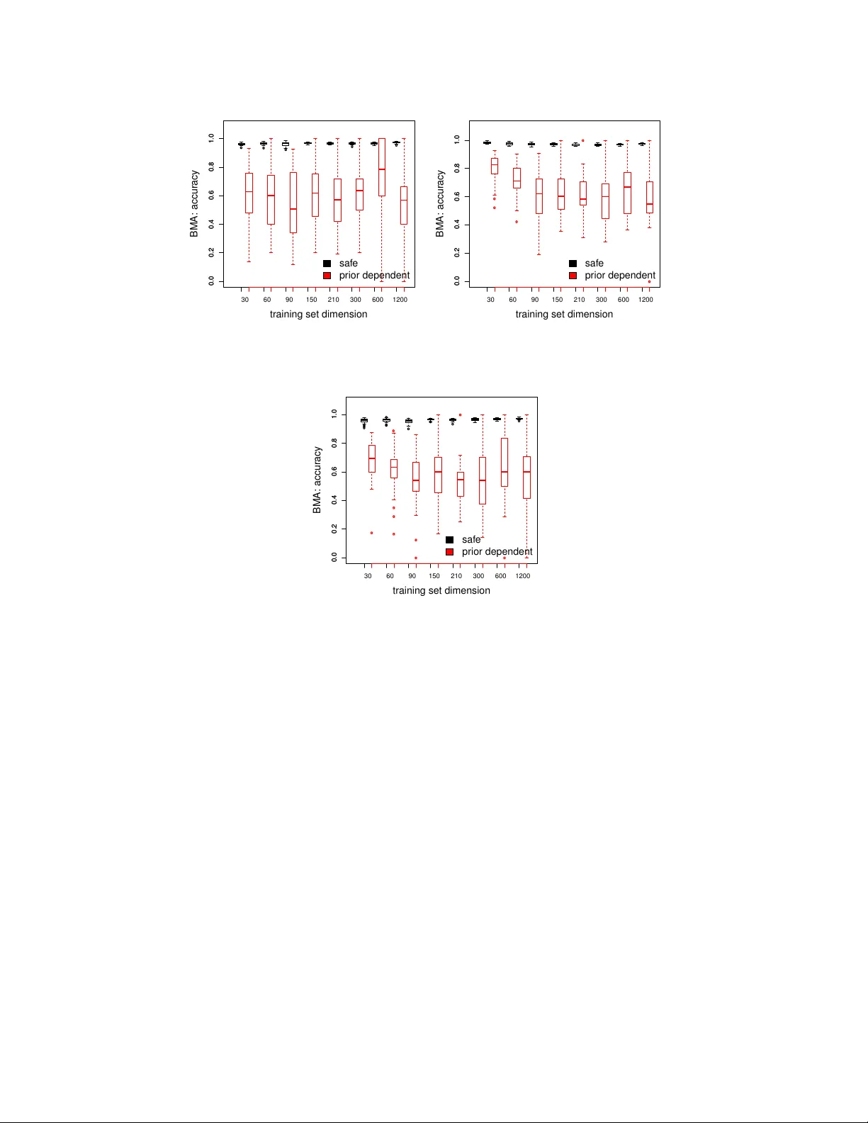
Credal Mo del Av eraging for classification: represen ting prior ignorance and exp ert opinions. Giorgio Corani a, ∗ , Andrea Mignatti b a Istituto Dal le Mol le di Studi sul l’Intel ligenza Artificiale (IDSIA) Gal leria 2, 6928 Manno (Lugano), Switzerland b Dip artimento di Elettr onic a, Informazione e Bioinge gneria Polite cnico di Milano, Italy Abstract Ba yesian model a veraging (BMA) is the state of the art approach for o vercoming model uncertain ty . Y et, esp ecially on small data sets, the results yielded b y BMA might be sensitiv e to the prior o ver the models. Credal Model Av eraging (CMA) addresses this problem by substituting the single prior ov er the mo dels by a set of priors (credal set). Suc h approac h solv es the problem of ho w to c ho ose the prior ov er the mo dels and automates sensitivit y analysis. W e discuss v arious CMA algorithms for building an ensemble of logistic regressors characterized by different sets of cov ariates. W e show ho w CMA can b e appropriately tuned to the case in which one is prior-ignorant and to the case in whic h instead domain knowledge is av ailable. CMA detects prior-dep endent instances, namely instances in whic h a different class is more probable dep ending on the prior ov er the mo dels. On suc h instances CMA susp ends the judgment, returning multiple classes. W e thoroughly compare differen t BMA and CMA v ariants on a real case study , predicting presence of Alpine marmot burrows in an Alpine v alley . W e find that BMA is almost a random guesser on the instances recognized as prior-dep enden t b y CMA. 1. In tro duction Classific ation is the problem of predicting the outcome of a categorical v ariable on the basis of several v ariables (called fe atur es or c ovariates ). Ho wev er, there is often considerable uncertaint y ab out whic h cov ariates should b e included in the classifier. T ypically different sets of cov ariates are plausible giv en the av ailable data. In this case dra wing conclusions on the basis of the supp osedly b est single mo del can lead to o verconfiden t conclusions, o verlooking the uncertaint y of mo del selection ( mo del unc ertainty ). Ba yesian mo del a veraging (BMA) [9] is a principled solution to mo del uncertain ty . BMA com bines the inferences of multiple mo dels; the w eights of the com bination are the mo dels’ p osterior probabilities. Ho wev er the results of BMA can b e sensitive on the prior probabilit y assigned to the differen t mo dels. A common approach is to assign equal prior probability to all models ( uniform prior ). A more sophisticated solution is to adopt a hier ar chic al prior o ver the mo dels, which yields inferences less sensitive of the choice of the prior parameters [4, 11]. Ho wev er the sp ecification of any prior implies some arbitrariness, whic h can lead to risky conclusions; such risk is esp ecially present on small data sets. Often BMA studies [20, 12] rep ort a sensitivity analysis, presenting the results obtained considering differen t priors ov er the mo dels. T o robustly deal with the sp ecification of the prior ov er the mo dels, we adopt a set of priors ( cr e dal set ) ov er the mo dels. W e th us adopt the paradigm of cr e dal classifiers [21] whic h extend traditional classifiers by considering sets of probability distributions. The main characteristic of credal classifiers is that they allow for set-v alued predictions of classes, when returning a single class is not deemed safe. Credal classifiers hav e b een developed in the area of imprecise probabilit y [19]. Cr e dal mo del aver aging (CMA) [6] generalizes BMA by substituting the prior ov er the mo dels b y a credal set. CMA thus combines a set of traditional classifiers using imprecise probability . CMA was firstly in tro duced [6] to create an imprecise ensemble of naive Ba yes classifiers. CMA adopts the credal set to express weak b eliefs ab out the mo del prior probabilities: b y doing so, it do es not commit to a single prior ov er the mo dels. As it is t ypical of credal classifiers, CMA compute inferences which return interval probabilities rather than single probabilities. F or example, when classifying an instance CMA computes the upp er and the lower posterior probability of eac h class. ∗ Corresponding author Email addr esses: giorgio@idsia.ch (Giorgio Corani), andrea.mignatti@polimi.it (Andrea Mignatti) The length of the interv al shows the sensitivit y of the p osterior on the prior ov er the mo dels, automating sensitivity analysis. CMA identifies prior-dep endent instances, namely instances in which a different class is more probable dep ending on the prior ov er the mo dels. In Corani and Mignatti [5] we studied the problem of robustly predicting the presence of Alpine marmot ( Mar- mota marmota ) on the basis of several en vironmen tal cov ariates (slop e, altitude, etc.). Ba yesian mo del a veraging of logistic regressors is the state of the art approac h for analyzing presence/absence data [20, 12, 17]. W e thus devised [5] CMA for logistic regression considering a constrained class of priors o ver the mo dels which allow ed for an analytical solution of the optimization problems. The credal set of CMA mo deled a condition close to prior near- ignorance. Moreov er we presented some preliminary results on the data set of presence of Alpine marmot collected b y AM. In particular we compared CMA against the BMA induced using the uniform prior ov er the mo dels. In this pap er w e extend in several resp ects our previous w ork. F rom the algorithmic viewp oin t we consider a more general class of distributions for the prior probability of the mo dels. The new class of priors is a straightforw ard generalization of the previous one; yet it allows representing prior knowledge in a muc h more flexible wa y . As a side-effect, the new class of priors requires a numerical solution of the optimization problems. W e discuss three differen t CMA v ariants. The first is our previous algorithm [5]. The new algorithm based on the more general class of priors yields t wo v ariants: one referring to prior ignorance and one referring to partial prior kno wledge. T o elicit prior kno wledge we interview ed three experts: tw o scientists who published several pap ers on the sp ecies and a master student who participated in the collection of marmot data without analyzing them. W e present also a muc h extended empirical analysis of the Alpine marmot. W e consider the three men tioned CMA v ariants and three BMA v arian ts, which differ in the prior ov er the mo dels. Tw o priors are non-informativ e (uniform and hierarc hical); the third prior is instead based on the exp ert statemen ts and is thus informative. W e assess not only the classification performance but also another important inference, namely the posterior probabilit y of inclusion of the cov ariates. The pap er is organized as follows: Section 2 and 3 present the BMA and CMA algorithms; Section 4 describ es the case study of Alpine marmot and the interview of the exp erts; Section 5 presents the empirical results. 2. Logistic regression and Bay esian mo del av eraging The goal is to predict the outcome of the binary class v ariable C whic h can assume v alues c 0 or c 1 . There are k c ovariates { X 1 , X 2 , . . . X k } ; an observ ation of the set of cov ariates is x = { x 1 , . . . , x k } . Giv en k cov ariates, 2 k differen t subsets of co v ariates can b e defined; each subset of cov ariates yields a mo del structur e (or, more concisely , a structur e ). W e denote by m i the i- th mo del structure, by X i its set of cov ariates and by P ( m i | D ) its p osterior probabilit y . A training set of size D is a v ailable for learning the mo dels. The data set has size n , namely it contains n joint observ ations of the co v ariates and the class. W e denote as P ( c 1 | D , x , m i ) the p osterior probability of c 1 giv en the co v ariate v alues x and the mo del m i whic h has b een trained on data set D . The logistic regression mo del is: η D, x ,m i = log  P ( c 1 | D , x , m i ) 1 − P ( c 1 | D , x , m i )  = β 0 + X X l ∈X i β l x l (1) where η D, x ,m i denotes the lo git of the p osterior probability of presence, x l the observ ation of l -th cov ariate which has b een included in mo del m i and β l its co efficien t. BMA addresses mo del uncertaint y by combining the inferences of multiple mo dels, and w eighting them b y the mo dels’ posterior probability . The p osterior probabilit y of presence is thus obtained b y marginalizing out the mo del v ariable [9]: P ( c 1 | D , x ) = X m i ∈M P ( c 1 | D , x , m i ) P ( m i | D ) (2) where M denotes the mo del space, which con tains the 2 k logistic regressors obtained considering all the p ossible subsets of features. The p osterior probability of m i giv en the data is computed as follows: P ( m i | D ) = P ( m i ) P ( D | m i ) P m i ∈M P ( m i ) P ( D | m i ) (3) where P ( m i ) and P ( D | m i ) are resp ectiv ely the prior probabilit y and the mar ginal likeliho o d of mo del m i . The marginal lik eliho o d integrates the likelihoo d with resp ect to the mo del parameters: P ( D | m i ) = ˆ P ( D | m i , β i ) P ( β i | m i ) d β i 2 where β i denotes the set of parameters of mo del m i . A conv enient approximation for computing the mo dels’ marginal lik eliho od is based on the BIC [15]. The BIC of mo del m i is BIC i = − 2 LL i + | β i | log( n ) (4) where LL i denotes the log-likelihoo d of m i , | β i | the n umber of its parameters and n the num b er of data p oin ts on the data set. The marginal lik eliho o d of mo del m i can b e approximated as: P ( D | m i ) ≈ exp( − B I C i / 2) P m i ∈M exp( − B I C i / 2) . (5) This approximation is conv enient from a computational viewp oin t and generally accurate; therefore, it is often adopted to compute BMA [15, 20, 12]. Using the BIC approximation it is no longer necessary sp ecifying the prior probabilit y P ( β i | m i ) of the mo del parameters. The p osterior probability of mo del m i is then appro ximated as: P ( m i | D ) ≈ exp( − B I C i / 2) P ( m i ) P m i ∈M exp( − B I C i / 2) P ( m i ) . (6) A large num b er of co v ariates implies a huge mo del space, making it necessary to appro ximate the summation of Eqn. (2); computational strategies to this end are discussed for instance by [4]. Ho wev er our exp erimen ts inv olve a limited n umber of cov ariates and thus we exhaustively sample the mo del space. Often one is interested in the p osterior probability of inclusion of feature X j . This is the sum the p osterior probabilities of the mo del structures which do include X j : P ( β j 6 = 0) = X m i ∈M ρ ij P ( m i | D ) (7) where the binary v ariable ρ ij is 1 if mo del m i includes co v ariate X j and otherwise. 2.1. Non-informative prior over the mo dels A simple approac h to set the prior probability of the mo dels is the indep endent Bernoul li prior (IB prior). The IB prior assumes that each co v ariate is indep enden tly included in the mo del with identical probability θ [4]. Denoting by k i the num b er of cov ariates included by mo del m i and by k the total num b er of co v ariates, the prior probabilit y of mo del m i is : P ( m i ) = θ k i (1 − θ ) k − k i (8) whic h dep ends on the single parameter θ . By setting θ =1/2 one obtains the uniform prior over the mo dels , which assigns to eac h mo del equal probabilit y 1 / 2 k . Ho wev er the uniform prior is quite informative if analyzed from the viewp oin t of the mo del size , namely the n umber of cov ariates included in the mo del. W e denote the mo del size b y W . The IB prior implies W to b e binomially distributed: W ∼ B in ( θ , k ) [11]. As well-kno wn, the binomial distribution is far from flat. A flat prior distribution ov er the mo del size can b e obtained by adopting the Beta-Binomial (BB) prior [11, 4]. Compared to the IB prior, the BB prior yields p osterior inferences which are less sensitive on the v alue of θ . The BB has b een recently recommended also for handling the problem of multiple hypothesis testing [16, 3]. The BB prior treats the parameter θ as a random v ariable with Beta prior distribution: θ ∼ B eta ( α, β ). It is common to set α = β = 1; under this choice, the Beta distribution is uniform . The resulting probability of mo del m i whic h contains k i co v ariates is [11]: P ( m i ) = k i !( k − k i )! k + 1! (9) The resulting probabilit y of the mo del size W to b e equal to k i is: P ( W = k i ) = 1 k + 1 ∀ m i (10) The mo del size is thus uniformly distributed, as a result of having set a uniform prior on θ . In the App endix we sho w the analytical deriv ation of formulas (9)–(10). Summing up, the IB prior under the choice θ = 1 / 2 implies all mo dels to b e equally probable and the mo del size to be binomially distributed. Instead the BB prior under the c hoice α = β = 1 implies the probability of eac h mo del to dep end on the num b er of cov ariates according to Eqn.(9) and the mo del size W to b e uniformly distributed. In Fig.1 we compare the prior distribution on the mo del size W obtained using the IB and the BB prior for k =6; this is the num b er of cov ariates of our case study . 3 0 1 2 3 4 5 6 0 0 . 1 0 . 2 0 . 3 W Probability mass function BB prior ( α = β = 1) IB prior ( θ =0.5) Figure 1: Prior distribution on the mo del size, under the indep enden t Bernoulli and the b eta-binomial prior for k =6. 2.2. Informative prior One can express domain knowledge by differently sp ecifying the prior probability of inclusion of eac h cov ariate. This requires generalizing the IB prior so that each cov ariate has its own prior probability of inclusion. W e denote b y θ the [ k × 1] vector including the prior probability of inclusion of cov ariates X 1 , . . . , X k and by θ j the probability of inclusion of the single co v ariate X j . The prior probability of mo del m i is th us: P ( m i ) = Y X j ∈X i θ j Y X j 6∈X i (1 − θ j ) (11) where we recall that X i is the set of cov ariates included in mo del m i . W e call this prior NB, which stands for N on- iden tical B ernoulli. The NB prior generalizes the IB prior, retaining its indep endence assumption but removing the constrain t of the prior probability of inclusion b eing equal for all cov ariates. 3. Credal Mo del Av eraging (CMA) CMA generalizes BMA by substituting the prior ov er the mo dels by a set of priors ov er the mo dels. The set of priors is called cr e dal set [21]. W e discuss t wo differen t v ersions of CMA: CMA ib and CMA nb . CMA ib [5] generalizes BMA induced under the IB prior; CMA nb generalizes BMA induced under the NB prior. 3.1. CMA ib W e start b y presenting CMA ib . The BMA induced under the IB prior requires sp ecifying a single v alue of θ ; instead CMA ib allo ws θ to v ary within the interv al [ θ , θ ]. The constraints θ > 0 and θ < 1 apply to the credal set of CMA ib . F or instance, the IB prior with θ =0 assigns zero prior probability to each mo del apart from the nul l model whic h includes no cov ariates. The problem is that suc h sharp zero probabilities do not change after having seen the data: prior and p osterior probabilities of the mo dels remain identical. In other words, such prior preven ts learning from data. In the same wa y the IB prior with θ = 1 preven ts learning from data. The IB priors with θ = 0 and θ = 1 are thus excluded from the credal set. CMA ib represen ts a condition close to W alley’s prior near-ignorance [19, Chap.5.3.2] if one sets θ =  and θ = 1 −  . This is the approach follow ed in [5]. The inferences of CMA ib return intervals of probability rather than a single probability . F or instance CMA ib computes an interval for the p osterior probabilit y of each class. The interv al shows the sensitivity of the p osterior probabilit y on the prior ov er the mo dels. Thus, CMA ib automates sensitivit y analysis. The lower p osterior probabilit y of class c 1 is computed as follo ws: P ( c 1 | D , x ) = min θ ∈ [ θ ,θ ] X m i ∈M P ( c 1 | D , x , m i ) P ( m i | D ) = min θ ∈ [ θ ,θ ] X m i ∈M P ( c 1 | D , x , m i ) P ( D | m i ) P ( m i ) P m j ∈M P ( D | m j ) P ( m j ) = min θ ∈ [ θ ,θ ] X m i ∈M P ( c 1 | D , x , m i ) P ( D | m i ) θ k i (1 − θ ) k − k i P m j ∈M P ( D | m j ) θ k j (1 − θ ) k − k j (12) 4 where the marginal likelihoo ds P ( D | m i ) are computed using the BIC approximation of Eqn.(5). The upp er proba- bilit y of c 1 is obtained b y maximizing rather than minimizing expression (12). Since our problem has only tw o classes, the upp er and lo wer p osterior probability of c 0 are readily obtained as: P ( c 0 | D , x ) = 1 − P ( c 1 | D , x ) P ( c 0 | D , x ) = 1 − P ( c 1 | D , x ) Another relev ant inference is the p osterior probability of inclusion of a cov ariate. F or instance, the lower probabilit y of inclusion of cov ariate X j is: P ( β j 6 = 0) = min θ ∈ [ θ ,θ ] X m i ∈M ρ ij P ( m i | D ) = min θ ∈ [ θ ,θ ] X m i ∈M ρ ij P ( D | m i ) P ( m i ) P m j ∈M P ( D | m j ) P ( m j ) = min θ ∈ [ θ ,θ ] X m i ∈M ρ ij P ( D | m i ) θ k i (1 − θ ) k − k i P m j ∈M P ( D | m j ) θ k j (1 − θ ) k − k j (13) where the binary v ariable ρ ij is 1 if mo del m i includes co v ariate X j and 0 otherwise. All suc h optimization problems are solved by the analytical pro cedures rep orted in the App endix. 3.2. CMA nb CMA nb generalizes BMA induced under the NB prior. As describ ed in Sec. 2.2, the NB prior allo ws sp ecifying a different prior probability for each co v ariate. CMA nb p ermits also to sp ecify a different upp er and lower prior probabilit y of inclusion for each cov ariate. W e denote by θ j and θ j the upp er and low er prior probabilit y of X j . Moreo ver, we denote by θ and θ the vectors collecting the upp er and low er probabilities of all cov ariates. As in the case of CMA ib , the probability of inclusion cannot b e exactly zero or one. A condition close to prior ignorance can b e mo deled by setting for all cov ariates θ j =  and θ j = 1 −  . Let us denote by K ( θ ) the credal set which con tains the admissible v alues for θ . The credal set K ( θ ) is largely differen t b et ween CMA nb and CMA ib . Consider a case with three co v ariates, in whic h we w ant to model a condition of ignorance. Using  = 0 . 05, under CMA ib w e would set θ =0.05 and θ =0.95. The credal set K ( θ ) of CMA ib w ould hav e tw o extreme p oin ts: { 0 . 05; 0 . 05; 0 . 05 } ; { 0 . 95; 0 . 95; 0 . 95 } . The credal set K ( θ ) of CMA nb w ould hav e 2 3 =8 extreme points: the tw o extreme p oints of CMA ib and 6 further ones, suc h as for instance { 0 . 05; 0 . 95; 0 . 05 } , { 0 . 95; 0 . 95; 0 . 05 } and so on. The c hoice  = 0 . 05 is a compromise b et ween the ob jectiv e of representing prior ignorance while not getting to o close to 0 and 1. The function f ( θ ) which represents how the p osterior probability of inclusion v aries as a function of θ is contin uous. It takes v alue 0 for θ =0 and v alue 1 for θ =1. Thus, it usually has large curv ature near θ =0 and θ =1. V ery small v alues of epsilon w ould return large CMA in terv als, even if the p osterior v aries narrowly in most of the in terv al. The upp er and low er probabilities are computed by solving an optimization in a k -dimensional space. The low er p osterior probability of c 1 is: P ( c 1 | D , x ) = min θ ∈ [ θ , θ ] X m i ∈M P ( c 1 | D , x , m i ) P ( m i | D ) = min θ ∈ [ θ , θ ] X m i ∈M P ( c 1 | D , x , m i ) P ( D | m i ) P ( m i ) P m j ∈M P ( D | m j ) P ( m j ) = min θ ∈ [ θ , θ ] X m i ∈M P ( c 1 | D , x , m i ) P ( D | m i ) Q X j ∈X i θ j Q X j 6∈X i (1 − θ j ) P m j ∈M P ( D | m j ) Q X j ∈X i θ j Q X j 6∈X i (1 − θ j ) (14) Also for CMA nb the upp er and low er probability of c 0 are the complement to 1 of the low er and upp er probability of c 1 . 5 The lo wer p osterior probability of inclusion of cov ariate X j is: P ( β j 6 = 0) = min θ ∈ [ θ , θ ] X m i ∈M ρ ij P ( m i | D ) = min θ ∈ [ θ , θ ] X m i ∈M ρ ij P ( D | m i ) P ( m i ) P m j ∈M P ( D | m j ) P ( m j ) = min θ ∈ [ θ , θ ] X m i ∈M ρ ij P ( D | m i ) Q X j ∈X i θ j Q X j 6∈X i (1 − θ j ) P m j ∈M P ( D | m j ) Q j ∈X i θ j Q X j 6∈X i (1 − θ j ) (15) where ρ ij is set to 1 if the co v ariate X j is included in the mo del m i and to 0 otherwise. The optimization problems of CMA nb cannot b e solved analytically; we thus rely on numerical optimization. In particular we adopt a lo cal solv er pro vided b y the NLopt soft ware ( http://ab- initio.mit.edu/nlopt ). W e use the nloptr pac k age 1 as in terface b et ween R and NLopt . W e compute the gradient of the ob jective function through the sym b olic solv er of R and then we provide it to the solver. 3.3. Sampling the mo del sp ac e CMA has b een describ ed so far assuming to exhaustiv ely explore the mo del space. How ever, data sets with large n umber of cov ariates prev ent this approach. In this case it is necessary to sample the mo del space. Strategies suitable to sample the mo del space are discussed for instance in [4, 2]. The CMA algorithms can easily accommo date a set of sampled mo dels. Denote the set of sampled mo dels b y M 0 . The CMA inferences could b e p erformed using the formulas given in Sections 3.1 and 3.2, pro vided that the whole mo del space M is substituted by the sampled mo del space M 0 when summing o ver the mo dels. 3.4. T aking de cisions Tw o criteria are commonly used for classification under imprecise probability: interval-dominanc e and maxi- mality [18]. According to in terv al-dominance, class c 1 dominates c 2 (giv en cov ariates x ) if: P ( c 1 | D , x , θ ) > P ( c 2 | D , x , θ ) (16) According to maximalit y , class c 1 dominates c 2 iff: P ( c 1 | D , x , θ ) > P ( c 2 | D , x , θ ) ∀ θ ∈ [ θ , θ ] (17) If a class is interv al-dominan t it also maximal [18], but not vice versa. Th us interv al-dominance generally return more cautious classifications (more output classes) than maximality . Y et, if the class v ariable is binary the t w o criteria are equiv alent. This is prov en by the following lemma. Lemma 3.1. If the class variable is binary, maximality implies interval-dominanc e. Pro of F or a binary class v ariable: P ( c 1 | D , x , θ ) = 1 − P ( c 0 | D , x , θ ) Plugging this expression in Eqn.(17), w e get: P ( c 1 | D , x , θ ) > 1 / 2 ∀ θ ∈ [ θ , θ ] whic h implies: P ( c 0 | D , x , θ ) < 1 / 2 ∀ θ ∈ [ θ , θ ] Th us, P ( c 1 | D , x , θ ) > 1 / 2 (18) P ( c 0 | D , x , θ ) < 1 / 2 (19) so that P ( c 1 | D , x , θ ) > P ( c 0 | D , x , θ ).  1 http://cran.r- project.org/web/packages/nloptr/index.html 6 Th us when dealing with a binary class (like in our case study), maximality and interv al-dominance are equiv alent. F or instance, CMA returns c 1 as a prediction if b oth its upp er and low er p osterior probability are gr e ater than 1/2. In this case the instance is safe : the most probable class do es not v ary with the prior ov er the mo dels. Instead, CMA returns the set of classes { c 0 , c 1 } if the p osterior probability interv als of the tw o classes ov erlap. This happ ens if b oth classes hav e upper probability gr e ater than 1/2 and low er probability smal ler than 1/2. In this case the instance is prior-dep endent : one class or the other is more probable dep ending on the prior o v er the mo dels. A final consideration regards the case in whic h the prior used to induce BMA is included in the credal set of CMA. In this case the p osterior probability computed by BMA is included within the p osterior interv al computed b y CMA. When CMA returns a single class, BMA and CMA predictions match. 4. Case study Data regarding the distribution of Alpine marmot ( marmota marmota ) burro ws w ere collected by AM and other collab orators in the summer of 2010 and 2011, in an Alpine v alley in Northern Italy . T o dev elop the sp ecies distribution model we divide the explored area in to cells of 10 x 10m, obtaining a data set of 9429 cells. The fraction of presence ( pr evalenc e ) is 436/9429= 0.046. Considering that the Alpine marmot prefers south-facing slop es ranging b et w een 1600 and 3000 m a.s.l. [13], w e introduce altitude and slop e as cov ariates. A third relev ant piece of information is the asp ect, namely the angle b et ween the maxim um gradient of the terrain and the North. W e represen t the aspect by in tro ducing t wo co v ariates ( northitude and e astitude ), corresp onding resp ectiv ely to the cosine and the sine of the asp ect. Northitude and the eastitude are proxies for the amount and the temp oral distribution of sunlight received during the day . The fifth co v ariate is the curvatur e , which measures the upw ard con vexit y (or conca vity) of the terrain. The sixth and last co v ariate is the soil c over , namely the prop ortion of terrain not co vered by vegetation. W e obtain the soil cov er from a digital map of the land use 2 . The Alpine marmot is a mobile sp ecies, which uses a huge territory for its activities. Therefore the decision of establishing a burrow dep ends also on the conditions of the surrounding cells. F or this reason we av erage the v alue of eac h cov ariate ov er a circular buffer ar e a of 2 ha around the cell b eing analyzed. 4.1. Interviewing exp erts W e asked three exp erts for the prior probability of inclusion of eac h co v ariate; the results are rep orted in T able 1. The p o ol of exp erts is comp osed by tw o scientists who published sev eral pap ers on the sp ecies (Dr. Bernat Claram unt L´ op ez and Prof. W alter Arnold) and a master student (Mrs. Viviana Brambilla) who participated to the collection of marmot data without analyzing them. The prior b eliefs of the exp erts are shown in T able 1. The lab els of first, second and third exp ert are randomly assigned to hide whose are the prior b eliefs. The first exp ert provided us with a single probability v alue for each cov ariate, while the tw o other exp erts pro vided us with in terv al probabilities. The third exp ert provides in terv als strongly skew ed either tow ards inclusion or exclusion. Exp erts Priors First Exp ert Second Exp ert Third Exp ert CMA BMA (con vex hull) (cen tral p oin t) altitude 0.95 [0.80-0.95] [0.90-0.95] [0.80-0.95] 0.87 slop e 0.50 [0.70-0.95] [0.05-0.10] [0.05-0.95] 0.50 curvatur e 0.40 [0.40-0.60] [0.05-0.10] [0.05-0.60] 0.27 northitude 0.60 [0.60-0.80] [0.90-0.95] [0.60-0.95] 0.77 e astitude 0.60 [0.60-0.90] [0.05-0.10] [0.05-0.90] 0.50 soil c over 0.95 [0.70-0.95] [0.90-0.95] [0.70-0.95] 0.82 T able 1: Probability of inclusion according to the three exp erts; imprecise mo del of prior kno wledge (conv ex hull); precise model of prior knowledge (central p oint of the convex hull). W e aggregate in tw o different wa ys the exp ert b eliefs. Firstly we take their c onvex hul l in the spirit of imprecise probabilit y . W e will later use suc h con vex hulls to represen t (imprecise) prior knowledge within CMA nb , which 2 The database, known as DUSAF2.0, was retrieved at: http://www.cartografia.regione.lombardia.it/geoportale . 7 allo ws for different sp ecification of the low er and upp er prior probability of inclusion of eac h co v ariate. Secondly we tak e the c entr al p oint of the con vex hull in the more traditional spirit of representing prior knowledge b y a single prior distribution. W e will later use such information to design a NB prior for BMA. The difference among suc h t wo approaches can be readily appreciated. Consider slop e, for which the experts ha ve strongly different opinions. The con vex h ull of its prior probability of inclusion is a wide interv al (0.05–0.95), whic h appropriately represen ts a condition of substantial ignor anc e . The cen tral p oin t approac h yields prior probability of inclusion 0.5, whic h represents prior indiffer enc e ab out the inclusion/exclusion of the cov ariate. As p oin ted out b y [19, Chap.5.5], a mo del of prior indiffer enc e is inappropriate to mo del the substan tial uncertaint y which instead c haracterizes a state of ignor anc e . 5. Results W e induce BMA under three priors: IB ( θ =0.5, non-informativ e); BB ( α = β = 1, non-informativ e); NB (informativ e). W e call these three mo dels BMA ib , BMA bb and BMA nb . F or BMA nb w e set the prior probability of inclusion of each cov ariate equal to the central point of the con vex hull of the exp ert b eliefs rep orted in T able 1. Th us BMA nb em b o dies domain knowledge. W e also consider three v ariants of CMA. The first is CMA ib with θ = 0 . 95 and θ = 0 . 05. This is the mo del originally prop osed in Corani and Mignatti [5] and represents a condition close to prior-ignorance, though under the restrictive assumption of the prior probability of all cov ariates b eing equal. The second is CMA nb with the prior-ignoran t configuration θ j = 0 . 05 and θ j = 0 . 95 for eac h cov ariate. As already discussed, the credal set of CMA nb con tains a m uch wider v ariety of priors compared to CMA ib ; th us w e exp ect CMA nb to be muc h more imprecise than CMA ib . The third mo del is CMA exp . This is a v ariant of CMA nb whic h embo dies partial prior knowledge: upper and lo wer probability of inclusion of each cov ariate corresp ond to the upper and low er bound of the con v ex hull of the exp ert b eliefs (T able 1). CMA exp consider narrow er prior interv al of inclusion for the cov ariates than CMA nb and th us it should be more determinate than CMA nb . This application sho ws ho w CMA can be easily tuned to represen t prior ignorance or prior kno wledge. 5.1. Posterior pr ob ability of inclusion of c ovariates W e induce the three BMAs and CMAs using the whole data set (9429 instances). T able 2 rep orts the p osterior probabilit y of inclusion of eac h co v ariate under the different mo dels. Suc h pos terior is a p oin t estimate for the BMAs and an interv al estimate for the CMAs. W e recall that the b eta-binomial prior is not included in the credal set of the CMAs: for this reason its estimate can lie outside of the CMA interv als. Co v ariate BMA CMA BMA ib BMA nb BMA bb CMA ib CMA nb CMA exp altitude 1.00 1.00 1.00 [1.00 - 1.00] [1.00 - 1.00] [1.00 - 1.00] slop e 1.00 1.00 1.00 [1.00 - 1.00] [1.00 - 1.00] [1.00 - 1.00] curv ature 0.02 0.02 0.01 [0.00 - 0.27] [0.00 - 0.39] [0.00 - 0.03] northitude 1.00 1.00 1.00 [1.00 - 1.00] [1.00 - 1.00] [1.00 - 1.00] eastitude 1.00 1.00 1.00 [1.00 - 1.00] [1.00 - 1.00] [1.00 - 1.00] soil co ver 0.97 0.99 0.94 [0.66 - 1.00] [0.55 - 1.00] [0.99 - 1.00] T able 2: Posterior probability of inclusion of each cov ariates estimated by differen t mo dels. The most imp ortan t v ariables are altitude, slop e, eastitude and northitude, whose p osterior probabilit y of inclusion is estimated as 1 by all the considered mo del. In particular the posterior probabilit y of inclusion of such co v ariates is not sensitiv e on the prior ov er the mo dels, also thanks to the h uge data set. Remark ably in this case the p osterior interv als of CMA collapse in to a single p oin t, low er and upp er p osterior probability of such cov ariates b eing b oth one. The results for curv ature are less unanimous. The BMAs recognize it as irrelev ant, estimating a p osterior probabilit y not larger than 0.02. Y et, the t wo CMAs induced under prior-ignorance (CMA ib and CMA nb ) achiev e a m uch less certain conclusions, estimating the upp er p osterior probability of inclusion as 0.3 or 0.4. This hardly allo ws to safely discard such cov ariate. Interestingly , CMA exp ac hieves a m uch sharp er conclusion, assigning to the curv ature an upp er p osterior probabilit y of inclusion of only 0.03, in line with the Bay esian mo dels. Thus CMA exp 8 ac hieves (on this large data set) conclusions which are as sharp as those of the Bay esian mo dels, but m uch safer as it do es not commit to a single prior. The soil co ver is recognized as relev an t by the BMAs, its p osterior probability of inclusion ranging betw een 0.94 and 0.99 dep ending on the prior ov er the mo dels. Y et, according to CMA ib and CMA nb its lower p osterior probabilit y of inclusion do es not exceed 0.7. Also in this case CMA exp ac hieves a m uch sharp er conclusion, assigning to soil co ver a p osterior probability comprised b et ween 0.99 and 1, further showing the b eneficial effect of prior kno wledge. The results presen ted so far are obtained using the en tire dataset for training the mo dels. It is ho wev er in teresting rep eating the analysis with smaller training sets, in whic h the choice of the prior ov er the mo dels is likely to hav e a greater effect. W e thus do wn-sampled the data set, creating data sets of size comprised b et ween n =30 and n =6000. The training sets are str atifie d : they contain the same prop ortion of presence of the original data set. 0 1 , 000 2 , 000 3 , 000 4 , 000 5 , 000 6 , 000 0 0 . 2 0 . 4 0 . 6 0 . 8 1 n Post. Prob. Inclusion CMA nb CMA exp (a) Posterior interv als: CMA exp vs CMA nb . 0 1 , 000 2 , 000 3 , 000 4 , 000 5 , 000 6 , 000 0 0 . 2 0 . 4 0 . 6 0 . 8 1 n Post. Prob. Inclusion CMA ib CMA exp (b) Posterior interv als: CMA exp vs CMA ib . Figure 2: Upp er and low er posterior probability of inclusion of altitude for different CMA and BMA mo dels. In Fig.2(a) and 2(b) we show as an example how the upp er and low er p osterior probabilit y of inclusion of the altitude co v ariate v aries with n . W e sho w the upper and lo wer probabilit y of inclusion computed b y different CMAs. The gap b etw een upp er and low er probability of inclusion narro ws down as the sample size increases, even tually con verging tow ards a punctual probability . The gap b etw een upp er and low er probability computed by CMA exp is generally narrow er than those of CMA nb and CMA ib . This is the b eneficial effect of exp ert kno wledge. The curv e are non-monotonic, probably b ecause we p erformed just once the whole pro cedure. Averaging ov er man y rep etitions would yield smo other curv es. 5.2. Comp aring CMA and BMA pr e dictions W e consider training sets with dimension comprised b et ween 30 and 1500. Beyond this size no significant changes are detected. F or each sample size we rep eat 30 times the pro cedure of i) building a training set b y randomly down-sampling the original data set; ii) training the different BMAs and CMAs; iii) assessing the mo del predictions on the test set, constituted by 1000 instances not included in the training set. T raining and test sets are str atifie d : they ha ve the same pr evalenc e (fraction of presence data) of the original data set. The most common indicator of p erformance for classifiers is the ac cur acy , namely the prop ortion of instances correctly classified using 0.5 as probability threshold. Accuracy ranges b et ween 0.93 and 0.97 dep ending on the sample size. The accuracies of the different BMAs are pretty close. Ho wev er, a skew ed distribution of the classes can misleadingly inflate the v alue of accuracy . If for instance a sp ecies is absent from 90% of the sites, a trivial classifier whic h alwa ys returning absence w ould achiev e 90% accuracy without providing an y information. The A UC (area under the receiv er-op erating curv e) [8] is more robust than accuracy , b eing insensitiv e to class unbalance. The A UC of a random guesser is 0.5; the AUC of a p erfect predictor is 1. Figure 3 shows the AUC of BMA using differen t priors o ver the models. The plots are truncated at n =600, since no further significant changes are observed going b ey ond this amoun t of data. Larger training sets allow to b etter learn the mo del and result in larger AUC v alues. The impact of the prior on AUC is quite thin. Overall, BMA p erforms well, its AUC b eing generally sup erior to 0.8. In this case study , the probabilit y of presence is m uc h lo wer than the probabilit y of absence. Another meaningful indicator of performance is thus the recall (p ercentage of existing burrows whose presence is correctly predicted). 9 0 100 200 300 400 500 600 0 . 8 0 . 85 0 . 9 n AUC BMA ib BMA bb BMA nb 0 100 200 300 400 500 600 0.05 0.10 0.15 n Recall BMA ib BMA bb BMA nb Figure 3: AUC and recall of BMA under different priors. The plots are truncated at n =600 since after this v alue no further change is observed. Each point represents the av erage ov er 30 exp erimen ts. The recall of BMA nb is consistently higher than that of the other BMAs (Figure 3b), thus b enefiting from exp ert kno wledge. Indicators such as precision and recall are used when the problem is cost-sensitive. 0.0 0.1 0.2 0.3 0.4 0.0 0.1 0.2 0.3 0.4 0.0 0.1 0.2 0.3 0.4 30 60 90 150 210 300 600 1200 training set dimension fraction of pr ior−dependent instances CMA nb CMA exp CMA ib Figure 4: F raction of prior-dep endent instances for the different CMA v ariants. F or each CMA v ariant and each training set dimension, a b ox and whisker plot is rep orted. The limit of the b o x represent the interquartile range, while the thick line inside the b o x is the median. The limits of the whisk er extend out of the box to the most extreme data point whic h is no more than 1.5 times the in terquartile range from the b o x. Poin ts that lay out of the whiskers are shown as circles. W e now analyze the CMA results. W e call indeterminate classifications the cases in which CMA susp ends the judgmen t returning both classes. The p ercen tage of indeterminate classifications ( indeterminacy ) of the differen t CMAs is shown in Fig.4. The indeterminacy consistently decreases with the sample size. This is the well-kno wn b eha vior of credal classifiers, whic h b ecome more determinate as more data are av ailable. CMA nb is the most indeterminate algorithm; CMA ib is the least indeterminate algorithm. The reason of this b ehavior lies in the differen t definition of the credal sets: while b oth algorithms aim at represen ting a condition close to prior-ignorance, the credal set of CMA nb con tains a muc h wider set of p riors and results in higher imprecision. In terestingly , CMA exp is much less indeterminate than CMA nb thanks to prior kno wledge. W e recall that any CMA algorithm divides the instances in to tw o groups: the safe and the prior-dep endent ones. CMA returns a single class on the safe instances and b oth classes on the prior-dep endent ones. W e therefore separately assess the accuracy of BMA on the safe and on the prior-dep enden t instances. This analysis is more meaningful when the prior used to induce BMA is included in the credal set of CMA. W e th us consider the follo wing pairs: BMA ib vs CMA ib ; BMA ib vs CMA nb ; BMA ib vs CMA exp . Figure 5 (a) compares the accuracy of BMA ib on the instances recognized as safe and prior-dep enden t b y CMA ib . On the prior-dep endent instances the accuracy of BMA ib sev erely drops, getting almost close to random guessing. On a data set with t wo classes, a random guesser achiev es accuracy 0.5; the av erage accuracy of BMA ib on the prior-dep enden t instances is 0.6. On the safe instances, the accuracy of BMA is abov e 90%. CMA ib th us uncov ers a small yet non-negligible set of instances (b etw een 2% and 8%) ov er whic h BMA ib p erforms p o orly b ecause of prior-dep endence. The phenomenon is already known in the literature of the credal classification [7, 6]. It has b een moreov er observed [6, 5] that such doubtful instances are hardly identifiable by lo oking at the BMA p osterior 10 0.0 0. 2 0.4 0 .6 0.8 1. 0 0.0 0. 2 0.4 0 .6 0.8 1. 0 tr aining set dime nsion BMA: accur acy 30 60 90 150 21 0 300 600 1200 saf e pr ior dependen t (a) BMA ib vs CMA ib . 0.0 0.2 0.4 0.6 0.8 1.0 0.0 0.2 0.4 0.6 0.8 1.0 tr aining set dime nsion BMA: accur acy 30 60 90 150 210 300 600 1200 saf e pr ior dependen t (b) BMA nb vs CMA nb . 0.0 0.2 0.4 0.6 0.8 1.0 0.0 0.2 0.4 0.6 0.8 1.0 tr aining set dime nsion BMA: accur acy 30 60 90 150 210 300 600 1200 saf e pr ior dependen t (c) BMA nb vs CMA exp . Figure 5: The accuracy of BMA sharply drops on the prior-dep enden t instances recognized by CMA. Each b o xplot refers to 30 experiments. The boxplots are computed as describ ed in the caption of Figure 4. The corresponding fraction of indeterminate predictions is shown in Figure 4. probabilities. Detecting prior-dep endence using BMA would require cross-chec king the predictions of many BMAs, eac h induced with a different prior ov er the mo dels. This is quite unpractical and is not usually done. In Figure 5(b) we compare the accuracy of BMA nb on the instances recognized as safe and as prior-dep enden t b y CMA nb . The prior of BMA ib is contained in the credal set of CMA nb . The results is qualitativ ely similar to the previous one, with a sharp drop of accuracy of BMA ib on the instances recognized as prior-dep endent by CMA ib . Y et, the accuracy of BMA on the prior-indep enden t instances is higher (ab out 70%) compared to the previous case, since CMA nb is much more indeterminate than CMA ib . Ev entually , we compare the accuracy of BMA nb on the instances recognized as safe and as prior-dep endent b y CMA exp . Note that the prior of BMA nb is included in the credal set of CMA exp . On av erage, the accuracy of BMA nb on the prior-dep enden t instances is ab out 60%. The situation is quite similar to the comparison of BMA ib and CMA ib . 5.3. Utility me asur es T o further compare the classifiers we adopt the utilit y measures introduced in [22], which we briefly describ e in the following. The starting p oint is the disc ounte d ac cur acy , which rewards a prediction containing m classes with 1 /m if it contains the true class and with 0 otherwise. Within a b etting framework based on fairly general assumptions, discounted-accuracy is the only score whic h satisfies some fundamen tal properties for assessing b oth determinate and indeterminate classifications. In fact, for a determinate classification (a single class is returned) discoun ted-accuracy corresponds to the traditional classification accuracy . Y et discoun ted-accuracy has severe 11 0 100 200 300 400 500 600 0 . 93 0 . 94 0 . 95 0 . 96 0 . 97 n Accuracy/Utility BMA (accuracy) CMA ib ( u 65 ) CMA ib ( u 80 ) 0 100 200 300 400 500 600 0 . 88 0 . 9 0 . 92 0 . 94 0 . 96 n Utility ( u 65 ) CMA exp CMA nb CMA ib 0 100 200 300 400 500 600 0 . 93 0 . 94 0 . 95 0 . 96 0 . 97 n Utility ( u 80 ) CMA exp CMA nb CMA ib Figure 6: Accuracies of BMA ib versus utility of CMA ib . The plot is truncated at n =600 since after this v alue no further change of accuracies is observed. shortcomings. Consider t wo medical doctors, do ctor r andom and do ctor vacuous , who should diagnose whether a patien t is he althy or dise ase d . Doctor r andom issues uniformly random diagnosis; do ctor vacuous instead alwa ys returns b oth categories, th us admitting to b e ignorant. Let us assume that the hospital profits a quan tity of money prop ortional to the discounted-accuracy achiev ed by its do ctors at each visit. Both do ctors ha ve the same exp e cte d discoun ted-accuracy for eac h visit, namely 1 / 2. F or the hospital, b oth doctors pro vide the same exp e cte d profit from eac h visit, but with a substantial difference: the profit of do ctor v acuous has no v ariance. Any risk-av erse hospital manager should thus prefer do ctor v acuous ov er do ctor random: under risk-av ersion, the exp ected utility increases with exp ectation of the rew ards and decreases with their v ariance [10]. T o mo del this fact, it is necessary to apply a utility function to the discounted-accuracy score assigned to each instance. W e designed the utilit y function according to [22]: the utility of a correct and determinate classification (discounted-accuracy 1) is 1; the utility of a wrong classification (discounted-accuracy 0) is 0; the utilit y of an accurate but indeterminate classification consisting of tw o classes (discounted-accuracy 0.5) is assumed to lie b et ween 0.65 and 0.8. Notice that, following the first t wo rules, the utilit y of a traditional classifier corresp onds to its accuracy . Tw o quadratic utility functions are deriv ed, passing resp ectiv ely through { u (0) = 0 , u (0 . 5) = 0 . 65 , u (1) = 1 } and { u (0) = 0 , u (0 . 5) = 0 . 8 , u (1) = 1 } , denoted as u 65 and u 80 resp ectiv ely . Utility of credal classifiers and accuracy of determinate classifiers can b e directly compared. Figure 6(a) compares the accuracy of BMA ib with the utility of CMA ib , considering b oth u 65 and u 80 as utility functions. In b oth cases the utilit y of CMA ib is higher than the accuracy of BMA ib ; the extension to imprecise probabilit y pro ves v aluable. The gap is narro wer under u 65 and larger under u 80 , as the latter function assigns higher v alue to the indeterminate classifications. Moreov er, the gap gets thinner as the sample size increases: as the data set gro ws large, CMA ib b ecomes less indeterminate and thus closer to BMA ib . In Figure 6(b) and 6(c) we compare the differen t CMAs using u 65 and u 80 . According to u 65 , the b est performing mo del is CMA ib , follow ed by CMA exp and by CMA nb . The function u 65 assign a limited v alue to the indeterminate classifications. Thus under this utility the most determinate algorithm (CMA ib ) achiev es the highest score; the least determinate (CMA nb ) ac hieves the low est score. The same situation is found under u 80 , but only for small sample sizes ( n < 60). F or larger n , CMA nb b ecomes the highest scoring CMA. The p oint is that CMA nb is the most imprecise mo del, and under u 80 the imprecision is highly rew arded. Dep ending thus on the considered utilit y function, a differen t v ariant of CMA achiev es the b est p erformance. These results are fully reasonable: each CMA provides a different trade-off b etw een informativeness and robust- ness. Moreo ver, the tw o utilit y function represen ts t wo quite differen t t yp es of risk av ersion. It can b e exp ected 12 that the they differently rank the v arious CMAs. Y et, it is somehow puzzling that CMA exp is never ranked as the top CMA, despite b eing the only algorithm which provides b oth a flexible mo del of prior and a robust elicitation of prior kno wledge. A partial explanation is that the utilit y measures are deriv ed assuming all the errors to b e equally costly . In a problem like ours missing a presence is likely to b e m uch costlier than missing an absence. Y et, there is currently no w ay to assess credal classifiers assuming unequal misclassification costs. 6. Conclusions BMA is the state of the art approach to deal with mo del uncertaint y . Y et, the results of the BMA analysis can w ell dep end on the prior whic h has b een se t ov er the mo dels, esp ecially on small data sets. T o robustly deal with this problem, CMA adopts a set of priors ov er the mo dels rather than a single prior. CMA automates sensitivity analysis and detects prior-dep enden t instances, on which BMA is almost random guessing. T o identify the prior-dep enden t instances without using CMA, one would need to cross-chec k the predictions of man y BMAs, each induced with a different prior ov er the mo dels. This would b e very unpractical. W e ha ve presen ted three different v ersions of CMA. They represen t differen t t yp es of ignorance or partial kno wledge a priori. Experiments show that extending BMA to imprecise probability is indeed v aluable. Ho wev er, deciding which v ariant of CMA p erforms b etter is not easy , partially b ecause the trade-off b et ween robustness and informativeness is a sub jective matter and partially b ecause there are currently no score for assessing credal classifiers when the cost of the misclassification errors are unequal. An in teresting av enue for future works is to develop CMA algorithms for the analysis of prior-data conflict. This approach would allo w for detecting ma jor discrepancies b et ween prior distribution and data, thus chec king automatically the soundness of the opinion of the exp erts. A recent prop osal for prior-data conflict in the con text of credal classification is discussed b y [14]. Ac kno wledgments W e are grateful to Dr. Bernat Claramun t L´ opez (Cen ter for Ecological Researc h and F orestry Applications, Unit of Ecology of the Autonomous Univ ersity of Barcelona), Prof. W alter Arnold (Universit y of V eterinary Medicine in Vienna) and Mrs. Viviana Brambilla (Master studen t at the Universidade T ecnica de Lisb oa) who provided us with their prior probability of inclusion of the cov ariates. The research in this pap er has b een partially supp orted by the Swiss NSF grants no. 200020-132252. The work has b een p erformed during Andrea Mignatti’s PhD, supp orted b y F ondazione Lom bardia p er l’Am biente (pro ject SHARE- Stelvio). W e are moreov er grateful to the anonymous review ers. App endix A: solution of the CMA optimization problems. W e show in the follo wing ho w to solv e the optimization problems (minimization and maximization) for IB-CMA. Let us define the k sets M 1 . . . M k whic h include all the mo dels containing resp ectiv ely { 1 , 2 , . . . , k } co v ariates. F or instance, M 2 con tains all the mo dels which include tw o cov ariates. The mo dels included in the same set hav e the same prior probabilit y; for instance the prior probability of a mo del b elonging to the set M j is θ j (1 − θ ) k − j . W e denote L j = P m i ∈M j P ( D | m i ). The definition of v ariable Z j dep ends instead on the problem b eing addressed, as detailed in the following table: Pr oblem Equation numb er Definition of Z j Lo wer/Upper prob. of presence (12) P m i ∈M j P ( c 1 | D , x ) P ( D | m i ) Lo wer/Upper prob. of inclusion of cov ariate X j (13) P m i ∈M j ρ ij P ( D | m i ) where the binary v ariable ρ ij is 1 if mo del m i includes the co v ariate X j and 0 otherwise. The function to b e optimized (minimized or maximized) can b e written as: h ( θ ) := P k j =0 θ j (1 − θ ) k − j Z j P k j =0 θ j (1 − θ ) k − j L j (.1) 13 In the in terv al [ θ, θ ], the maxim um and minimum of h ( θ ) should lie either in the b oundary points θ = θ and θ = θ , or in an internal p oint of the interv al in which the first deriv ative of h ( θ ) is 0. Let us in tro duce f ( θ ) = P k j =0 θ j (1 − θ ) k − j Z j and g ( θ ) = P k j =0 θ j (1 − θ ) k − j L j . The first deriv ative h 0 ( θ ) is: h 0 ( θ ) = f 0 ( θ ) g ( θ ) − f ( θ ) g 0 ( θ ) g ( θ ) 2 , (.2) where g ( θ ) is strictly p ositive because L j is a sum of marginal likelihoo ds. W e can therefore search the solutions lo oking only at the numerator f 0 ( θ ) g ( θ ) − f ( θ ) g 0 ( θ ), which is a p olynomial of degree k ( k − 1) and thus has k ( k − 1) solutions in the complex plain. W e are in terested only in the r eal solutions that lie in the interv al ( θ , θ ). Such solutions, together with the boundary solutions θ = θ and θ = θ , constitute the set of c andidate solutions . T o find the minimum and the maximum h ( θ ), we ev aluate h ( θ ) in each candidate solution p oint, and even tually we retain the minim um or the maximum among such v alues. App endix B: the b eta-binomial pri or for Ba y esian mo del av eraging. The Beta-binomial (BB) prior is discussed for instance by [1, Chap.3.2]. It treats parameter θ as a random v ariable with Beta prior distribution: θ ∼ B eta ( α , β ). The prior probability of model m i whic h includes k i co v ariates is obtained by marginalizing out the Beta distribution: P ( m i ) = ˆ 1 0 θ k i (1 − θ ) k − k i p ( θ ) dθ = ˆ 1 0 θ k i (1 − θ ) k − k i θ α − 1 (1 − θ ) β − 1 B ( α, β ) dθ = Γ( α + β ) Γ( α )Γ( β ) ˆ 1 0 θ α + k i − 1 (1 − θ ) β + k − k i − 1 dθ = Γ( α + β ) Γ( α )Γ( β ) Γ( α + k i )Γ( β − k i + k ) Γ( α + β + k ) where the last passage leading to Eqn..3 is explained considering that the Beta distribution integrates to 1: Γ( α + β + k ) Γ( α + k i )Γ( β − k i + k ) ˆ 1 0 θ α + k i − 1 (1 − θ ) β + k − k i − 1 dθ = 1 = ⇒ ˆ 1 0 θ α + k i − 1 (1 − θ ) β + k − k i − 1 dθ = Γ( α + k i )Γ( β − k i + k ) Γ( α + β + k ) Under the c hoice α = β = 1, the Beta distribution becomes uniform and the probabilit y of model m i whic h con tains k i co v ariates b ecomes: P ( m i ) = Γ( α + β ) Γ( α )Γ( β ) Γ( α + k i )Γ( β − k i + k ) Γ( α + β + k ) = Γ(2) Γ(1)Γ(1) Γ(1 + k i )Γ(1 − k i + k ) Γ(2 + k ) = k i ! k − k i ! k + 1! This gives the prior probability of a mo del with k i co v ariates. The probability of the mo del size W to b e equal to k i is obtained by com bining Eqn.(9) with the observ ation that that there are  k k i  mo dels whic h contain k i co v ariates: P ( W = k i ) = P ( m i ) ·  k k i  = k i ! k − k i ! k + 1! k ! k − k i ! k i ! = 1 k + 1 ∀ m i The mo del size is thus uniformly distributed, as a result of having set a uniform prior on θ . References [1] Bernardo, J.M., Smith, A.F., 2009. Ba yesian theory . John Wiley & Sons. [2] Boull ´ e, M., 2007. Compression-based av eraging of selective naive Bay es classifiers. The Journal of Mac hine Learning Researc h 8, 1659–1685. [3] Carv alho, C.M., Scott, J.G., 2009. Ob jective Bay esian model selection in gaussian graphical models. Biometrik a 96, 497–512. 14 [4] Clyde, M., George, E.I., 2004. Model uncertaint y . Statistical science , 81–94. [5] Corani, G., Mignatti, A., 2013. Credal mo del av eraging of logistic regression for mo deling the distribution of marmot burrows, in: Cozman, F., Denœux, T., Desterck e, S., Seidenfeld, T. (Eds.), ISIPT A’13: Pro ceed- ings of the Seven th International Symp osium on Imprecise Probability: Theories and Applications, SIPT A, Compi ` egne. pp. 233–243. [6] Corani, G., Zaffalon, M., 2008a. Credal Mo del Averaging: an extension of Bay esian model av eraging to imprecise probabilities. Pro c. ECML-PKDD 2008 (Eur. Conf. on Machine Learning and Knowledge Discov ery in Databases) , 257–271. [7] Corani, G., Zaffalon, M., 2008b. Learning reliable classifiers from small or incomplete data sets: the naive credal classifier 2. The Journal of Machine Learning Research 9, 581–621. [8] F aw cett, T., 2006. An introduction to ROC analysis. P attern recognition letters 27, 861–874. [9] Hoeting, J.A.M., C.T. Raftery , A.V., 1999. Bay esian model a veraging: A tutorial. Statistical Science 44, 382–417. [10] Levy , H., Marko witz, H.M., 1979. Appro ximating expected utility b y a function of mean and v ariance. The American Economic Review 69, 308–317. [11] Ley , E., Steel, M.F., 2009. On the effect of prior assumptions in Bay esian mo del av eraging with applications to gro wth regression. Journal of Applied Econometrics 24, 651–674. [12] Link, W., Bark er, R., 2006. Mo del w eights and the foundations of multimodel inference. Ecology 87, 2626–2635. [13] L´ op ez, B., Pino, J., L´ op ez, A., 2010. Explaining the successful introduction of the alpine marmot in the Pyrenees. Biological Inv asions 12, 3205–3217. [14] Masegosa, A.R., Moral, S., 2014. Imprecise probabilit y mo dels for learning m ultinomial distributions from data. applications to learning credal net works. In ternational Journal of Approximate Reasoning , –. [15] Raftery , A.E., 1995. Bay esian mo del selection in so cial research. Sociological metho dology 25, 111–164. [16] Scott, J.G., Berger, J.O., 2006. An exploration of asp ects of Bay esian multiple testing. Journal of Statistical Planning and Inference 136, 2144–2162. [17] Thomson, J.R., Mac Nally , R., Fleishman, E., Horro c ks, G., 2007. Predicting bird species distributions in reconstructed landscap es. Conserv ation Biology 21, 752–766. [18] T roffaes, M., 2007. Decision making under uncertain ty using imprecise probabilities. International Journal of Appro ximate Reasoning 45, 17–29. [19] W alley , P ., 1991. Statistical reasoning with imprecise probabilities. Chapman and Hall London. [20] Win tle, B., McCarthy , M., V olinsky , C., Kav anagh, R., 2003. The use of Ba yesian mo del av eraging to b etter represen t uncertaint y in ecological mo dels. Conserv ation Biology 17, 1579–1590. [21] Zaffalon, M., 2001. Statistical inference of the naiv e credal classifier, in: de Cooman, G., Fine, T.L., Seidenfeld, T. (Eds.), ISIPT A ’01: Pro ceedings of the Second In ternational Symposium on Imprecise Probabilities and Their Applications, pp. 384–393. [22] Zaffalon, M. , Corani, G., Maua, D., 2012. Ev aluating credal classifiers b y utilit y-discoun ted predictiv e accuracy . In ternational Journal of Approximate Reasoning 53, 1282 – 1301. 15